


Introduction
As part of the Ross Ice Shelf Geophysical and Glaciological Survey (RIGGS), 17 d.c. electrical resistivity profiles have been completed at 11 locations on the Ross Ice Shelf. During the first RIGGS season (1973–74) electrical resistivity measurements were made at the RIGGS base camp (station B.C.) (Reference BentleyBentley, 1977). A computer program was developed to calculate apparent resistivities on an ice shelf in which the density and temperature, and thus the resistivity, vary continuously with depth. Also, studies of the mass balance at the ice-water boundary beneath the ice shelf, upon which the englacial temperatures depend, were carried out. However, since neither the actual temperatures nor the activation energy were accurately known, the bottom balance-rate ![]() was difficult to evaluate. Measurements at station R.I. in 1974–75 yielded no new information on bottom balance-rates because of the discovery of highly resistive ice at the base of the shelf (Reference BentleyBentley, 1976). During the 1976–77 field season, drilling was completed down to a depth of 320 m at the RISP drill site (J-9) on the Ross Ice Shelf, about 30 km down-stream from station B.C. Temperature–depth measurements then became available for further investigations of the dependence of resistivity on temperature (Reference BentleyBentley, 1979).
was difficult to evaluate. Measurements at station R.I. in 1974–75 yielded no new information on bottom balance-rates because of the discovery of highly resistive ice at the base of the shelf (Reference BentleyBentley, 1976). During the 1976–77 field season, drilling was completed down to a depth of 320 m at the RISP drill site (J-9) on the Ross Ice Shelf, about 30 km down-stream from station B.C. Temperature–depth measurements then became available for further investigations of the dependence of resistivity on temperature (Reference BentleyBentley, 1979).
In 1976–77 and 1977–78, resistivity sounding was extended to eight other stations (Fig. 1). Density–depth information was obtained from seismic short-refraction shooting, and radar soundings yielded the ice thicknesses along the resistivity profiles. The measurements reported on here cover five of these stations (C-16, M-14, O-11, O-19, and Q-13), where the form of the apparent resistivity curves was relatively simple. Temperature–depth data were collected from 100 m drill holes at the two RIGGS base camps (C-16 and Q-13) and have kindly been made available to the authors in advance of publication (personal communications from C. C. Langway, Jr, and E. Chiang, 1978, and J. H. Cragin, 1977).

Fig. 1. Map of the Ross Ice Shelf, showing the locations and orientations of the resistivity profiles (![]() ). Solid arrows indicate measured flow directions (Reference SwithinbankSwithinbank, 1963; Reference Dorrer, Dorrer, Hofmann and SeufertDorrer and others, 1969; Reference ThomasThomas, 1976). Dashed arrows show inferred flow directions (Reference RobinRobin, 1975; Reference Bentley, Bentley, Clough, Jezek and ShabtaieBentley and others, 1979). Grid North is towards the top of the figure.
). Solid arrows indicate measured flow directions (Reference SwithinbankSwithinbank, 1963; Reference Dorrer, Dorrer, Hofmann and SeufertDorrer and others, 1969; Reference ThomasThomas, 1976). Dashed arrows show inferred flow directions (Reference RobinRobin, 1975; Reference Bentley, Bentley, Clough, Jezek and ShabtaieBentley and others, 1979). Grid North is towards the top of the figure.
Field Method and Results
The Schlumberger array configuration (Reference BentleyBentley, 1977) was used throughout the investigation. The current-electrode separation was increased to at least 500 m at all stations, and as far as 1000 m at station C-16. Two perpendicular profiles were completed at C-16 and at Q-13, one each at the other sites.
The current I was provided by dry-cell batteries supplying voltages up to 2.8 kV, and was measured with a Triplett d.c. ammeter. The potential difference V was measured with a battery-operated electrometer (Keithley Instruments, model 600A or 600B), having an input impedance greater than 1014Ω. Sections of copper pipe were used for electrodes. To reduce the contact resistance between the firn and the current electrodes salt solution was poured around the electrodes, multiple electrodes were used for the larger current-electrode spacings.
Data Analysis
A data set for a particular electrode spacing usually consisted of four to eight series of readings of the decay of V and I. The direction of current flow was reversed between consecutive series to counteract the polarization effect at the current electrodes. Background potentials were largely balanced by circuitry in the electrometer, and their effect was further reduced by correcting for open-circuit readings before and after each V-I series. Data were analyzed by plotting V versus I for each configuration of electrodes (see examples in Fig. 2a; see also Reference BentleyBentley, 1977, fig. 3). A straight line, forced through the origin, was fitted by least-square analysis to each set of data, the slope giving the resistance Ω of the ice for that particular configuration. The apparent resistivity ρ a is then given by ρ a ═ KΩ, where

a and b are current and potential electrode separations from the center respectively (see Reference BentleyBentley, 1977).

Fig. 2. Sample plots of observed potential difference V versus current I at C-16. × and ![]() (first quadrant) denote current flow in the “positive” direction; × indicates one reading and
(first quadrant) denote current flow in the “positive” direction; × indicates one reading and ![]() two or more readings plotted at the same point on the graph. Dots (single readings) and circles (multiple readings) denote current flow in the negative direction (plotted in the third quadrant). Superscripts +, —, and ± on the symbol Ω denote slopes determined from first-quadrant data only, third-quadrant data only, and the average of the two
two or more readings plotted at the same point on the graph. Dots (single readings) and circles (multiple readings) denote current flow in the negative direction (plotted in the third quadrant). Superscripts +, —, and ± on the symbol Ω denote slopes determined from first-quadrant data only, third-quadrant data only, and the average of the two ![]() , respectively. The subscript 0 indicates that the regression line was forced through the origin. The solid lines indicate regression lines with slopes as shown. The dashed lines are the extension of the Ω0
– and the Ω0
+ lines into the first and third quadrants, respectively, a (upper) is for a ═ 100 m, b ═ 20 m; b (lower) is for a ═ 900 m, b ═ 140 m.
, respectively. The subscript 0 indicates that the regression line was forced through the origin. The solid lines indicate regression lines with slopes as shown. The dashed lines are the extension of the Ω0
– and the Ω0
+ lines into the first and third quadrants, respectively, a (upper) is for a ═ 100 m, b ═ 20 m; b (lower) is for a ═ 900 m, b ═ 140 m.

Fig. 3. Electrical resistivity sounding curves obtained on the Ross Ice Shelf. Some of the curves are identified by station of observation (R.I., H-13, etc.). Each curve was fitted to the observed data by hand for illustration purposes.
If there was more than one point at the same current–electrode spacing, the weighted average apparent resistivity ρ a was calculated from the equation

the corresponding standard error estimate σ ρ being given by

where (ρ a)i and (σ ρ )i are individual apparent resistivities and standard errors, respectively.
General Features of the Resistivity Sounding Curves
The resistivity curves on the ice shelf may be divided into two main groups which differ at large electrode separations. At separations less than one or two hundred meters most of the curves are similar, showing three characteristic zones (Fig. 3). For a < 10 m, all the curves reflect the near-surface layer of seasonal temperature changes and local inhomogeneities. The second zone, from 10 to 100 m, reflects primarily the increasing density with depth in the upper 50 m of the ice shelf. The third zone, from 100 m to a distance which is, for most profiles, roughly equal to the ice thickness, is affected principally by the temperature gradient and the activation energy in the solid ice. At greater distances the two groups of curves diverge, “Type 1” (M-14, O-19, unlabelled curves) showing apparent resistivities that decrease rapidly with distance, owing to the high conduction in the sea-water beneath the ice shelf, and “Type 2” (R.I., H-13, L-4, N-19) showing instead an increasing apparent resistivity revealing a zone of highly resistive ice, presumably at the base of the ice shelf, in which the resistivity is substantially higher than in the ice above. Type 2 profiles are associated either with major ice streams from West Antarctica (L-4, R.I.) or large outlet glaciers from East Antarctica (H-13, N-19). In this paper we consider only Type 1 curves since they more clearly reflect englacial temperatures.
Analysis
Model resistivities were calculated using the computer program developed by Reference BentleyBentley (1977). The resistivity ρ was assumed to vary with temperature T according to an Arrhenius law with activation energy E:
where k is Boltzmann’s constant (8.62 × 10⁻⁵ eV K –1 ═ 1.38 × 10⁻²³ kJ mol–1 K–1). Temperatures were calculated from the steady-state model of Reference CraryCrary (1961):

where T
0 is the surface temperature, TH
the basal temperature (—2°C), α the thermal diffusitivity (taken to be 1.2 × 10⁻⁶ m2 s–1), ![]() the surface balance rate,
the surface balance rate, ![]() the basal balance-rate, and H the ice thickness. It is important to note that the use of a steady-state model implies that quantitative estimates of
the basal balance-rate, and H the ice thickness. It is important to note that the use of a steady-state model implies that quantitative estimates of ![]() refer to average values over a time interval comparable to the response time of the ice shelf to temperature changes at its base, that is, several hundred years.
refer to average values over a time interval comparable to the response time of the ice shelf to temperature changes at its base, that is, several hundred years.
Firn densities for each station were determined from seismic refraction shooting along the same lines as the resistivity profiles (Reference KirchnerKirchner, unpublished). For the influence of density upon resistivity, Looyenga’s equation (Reference LooyengaLooyenga, 1965) was used, leading to the relation
and

where ρ
f and ρ
i are the resistivities of firn and ice, respectively, and ν is the firn-ice density ratio (see Reference BentleyBentley, 1977, for a detailed discussion). The ice thickness H at each station was determined by radar sounding along each resistivity profile (authors’ unpublished data). Values for ![]() and T
0 were taken either from Reference Clausen and DansgaardClausen and Dansgaard (1977) or from pit studies during I.G.Y. traverses (Reference Crary, Crary, Robinson, Bennett and BoydCrary and others, 1962).
and T
0 were taken either from Reference Clausen and DansgaardClausen and Dansgaard (1977) or from pit studies during I.G.Y. traverses (Reference Crary, Crary, Robinson, Bennett and BoydCrary and others, 1962).
We have tried two simple models of the activation energy based on our previous field work (Reference BentleyBentley, 1977, Reference Bentley1979) and laboratory measurements by several others (see summary in Reference Glen and ParenGlen and Paren, 1975)

These two models were applied previously to observations at station B.C. and J-9 (RISP Drill Camp), the fit appearing somewhat better for E ═ 0.15 eV than for E ═ 0.25 eV (Reference Bentley, Bentley, Clough, Jezek and ShabtaieBentley, 1979). This is also true for almost all cases in this paper.
Recent chemical analysis on the ice-core samples from the RISP drill site (Reference Herron and LangwayHerron and Langway, 1979) showed an exponential decrease in sodium-ion concentration as a function of depth, from 100p.p.b. (parts per billion) at the surface to about 65 p.p.b. at a depth of 50 m, and to about 30 p.p.b. at 130 m. Similar results have been reported for the Little America V core by Langway and others (1974), except that the value obtained there for the surface concentration was about 480 p.p.b. Decrease in chemical content with distance from the ice front for sites on the Ross Ice Shelf have been reported by Reference Warburton and LinkletterWarburton and Linkletter (1977) and Reference Herron and LangwayHerron and Langway (1979). The latter report an observed six-fold decrease in average sodium concentration in surface snows from 600 p.p.b. at the ice front to 100 p.p.b. at the RISP drill site, 450 km from the ice front.
Reference Gross, Gross, Hayslip and HoyGross and others (1978) reported that, in solid ice, the resistivity is proportional to C –0.4, where C is the impurity concentration. These considerations led Reference Bentley, Bentley, Clough, Jezek and ShabtaieBentley (1979) to conclude that an activation energy of 0.15 eV (14 kJ mol–1) is probably only apparent and that the results at J-9 are consistent with a true value of 0.25 eV (24 kj mol–1) for the activation energy. If that is correct, then apparent activation energies around 0.15 eV (14 kJ mol–1) elsewhere on the ice shelf probably have a similar explanation.
Other factors, such as total gas content, ageing, grain size, and crystalline structure could conceivably cause variation of resistivity with depth. They have not been included in the current analysis because their effects are largely unknown (see Reference Bentley, Bentley, Clough, Jezek and ShabtaieBentley, 1979).
In order to obtain estimates of the bottom balance-rate ![]() for each station, we have treated E and
for each station, we have treated E and ![]() as parameters in the model curves. These model curves were matched to the observations at 200 m (sometimes 100 m) since we are concerned with effects in the solid ice at depths greater than 100m, and wish to avoid any consideration of fit in the density-dominated region of the ρ
a curves. The parameters of the best model fits are shown in Table 1.
as parameters in the model curves. These model curves were matched to the observations at 200 m (sometimes 100 m) since we are concerned with effects in the solid ice at depths greater than 100m, and wish to avoid any consideration of fit in the density-dominated region of the ρ
a curves. The parameters of the best model fits are shown in Table 1.
Table 1. Summary ofRIGGSresistivity stations, and parameters used tocalculate the best model fit to the data for each station

Station Q-13
The apparent resistivities measured on the two profiles are different for separations greater than 100 m (Fig. 4). Several models were tried; the two that matched “Profile 1” best are shown in the Figure. No model was found that matched “Profile 2” although the quality of the data for “Profile 2” is high (there are as many as five measurements, using different source voltages and potential-electrode separations, at some distances). The anisotropy is probably real and may be related to the buried rift zones known to occur within 3 km of Q-13 (authors’ unpublished radar profiling data).

Fig. 4. Plot of apparent resistivities for both profiles at station Q-13. The height of each symbol represents the standard deviation calculated from linear fits to plots like those in Figure 2. The solid curves are the calculated models described in the text, with E and ![]() H
as shown.
H
as shown.
Measured temperatures in the ice (personal communication from J. H. Cragin, 1977) are in good agreement with the calculated model E ═ E
3, ![]() (Fig. 5). Since this model also fits Profile 1, we prefer it for station Q-13.
(Fig. 5). Since this model also fits Profile 1, we prefer it for station Q-13.

Fig. 5. Calculated temperature-depth curves for station Q-13 corresponding to models shown in Figure 4. Solid dots indicate temperatures measured in the 100 m core hole at Q-13.
Station O-11
Several models with different set of parameters were tried; two, E ═ E
3, ![]() and E ═ E
2,
and E ═ E
2, ![]() ═ —0.5 m year–1 (i.e. 0.5 m year–1 melting), are shown with the measured apparent resistivities(Fig. 6). The former appears to fit somewhat better thanthe latter.
═ —0.5 m year–1 (i.e. 0.5 m year–1 melting), are shown with the measured apparent resistivities(Fig. 6). The former appears to fit somewhat better thanthe latter.

Fig. 6. Plot of apparent resistivity at station O-11. Solid curves are calculated models with parameters as shown.
Station M-14
Of the three model curves shown (Fig. 7), the one with E ═ E
2, ![]() fits the observed values best. Note the small effect ofa bottom freeze-rate as large as 0.4 m year–1, showing the poor sensitivity to positive values of
fits the observed values best. Note the small effect ofa bottom freeze-rate as large as 0.4 m year–1, showing the poor sensitivity to positive values of ![]() at stations where the ice is relatively thin and the relatively flat “third zone” of the apparent resistivity curve is short in length. A bottom freeze-rate of 1 m year–1 or so would be needed to yield a fit with E ═ E
3. Note, however, that Reference CraryCrary’s (1961) temperature model can no longer be applied quantitatively to resistivities when bottom freezing occurs because of the greatly reduced resistivity of saline ice (see the Discussion section below).
at stations where the ice is relatively thin and the relatively flat “third zone” of the apparent resistivity curve is short in length. A bottom freeze-rate of 1 m year–1 or so would be needed to yield a fit with E ═ E
3. Note, however, that Reference CraryCrary’s (1961) temperature model can no longer be applied quantitatively to resistivities when bottom freezing occurs because of the greatly reduced resistivity of saline ice (see the Discussion section below).

Fig. 7. Plot of apparent resistivity at station M-14. Solid curves are calculated models with parameters as shown.
Station C-16
The resistivity soundings made along two perpendicular profiles were nearly in agreement and were combined after the removal of an 11% average difference. The combined profile is shown in Figure 8, along with two model curves with the same activation energy E
3, one with ![]() ═ —0.5 m year–1 and the other with
═ —0.5 m year–1 and the other with ![]() H
═ 0. The latter model fits the observed values up to a separation of 300 m, but at greater distances the observed values of apparent resistivity are significantly high, so that no simple model fits.
H
═ 0. The latter model fits the observed values up to a separation of 300 m, but at greater distances the observed values of apparent resistivity are significantly high, so that no simple model fits.

Fig. 8. Apparent resistivity data from station C-16. Apparent resistivities for each profile were obtained using the Ω0 ± values (see Fig. 2), and then combined as discussed in the text. Solid curves are calculated models with parameters as shown. The ρa points shown with light bars at separations of 900 m and 1000 m come from only one of the two profiles at C-16.
Measured temperatures (personal communication from C. C. Langway, Jr, and E. Chiang, 1978) and the two temperature models are shown in Figure 9; clearly, the model with ![]() ═ 0 is in excellent agreement with the measured values (the slight displacement reflects an improper choice of T
0 in the model calculation which was carried out before the observations were available).
═ 0 is in excellent agreement with the measured values (the slight displacement reflects an improper choice of T
0 in the model calculation which was carried out before the observations were available).

Fig. 9. Calculated temperature–depth curves for station C-16 corresponding to models shown in Figure 8. Solid dots indicate temperatures measured in the 100 m core hole at C-16.
It is tempting to conclude that there is a highly resistive basal layer at the bottom of the ice shelf similar to, but thinner than, the one that presumably produced the “Type 2” curve at the mouth of Beardmore Glacier (station H-13), since C-16 lies on Beardmore Glacier ice directly down-stream (Reference Bentley, Bentley, Clough, Jezek and ShabtaieBentley and others, 1979). However, it is first necessary to examine the data collected at this station more carefully. At separations of 400 m and larger the points on the V-I plots deviate increasingly from well-defined straightlines (the worst case is shown in Fig. 2b; see also the well-defined line in Fig. 2a). The best-straight-line fit to the first-quadrant data deviates markedly from its constrained passage through the origin. The cause of this non-zero intercept is not known. To put the magnitude of thedeviation in perspective, first-and third-quadrant data were fitted with separate regression lines that were not forced through origin. Calculating apparent resistivity from the third-quadrant slopes yielded results not much different from Figure 8, but use of the first-quadrant slopes cause a large decrease in the observed values (Fig. 2b), enough to bring them into agreement with the model curves (Fig. 10). Although we know of no valid experimental reason for accepting the first-quadrant slopes rather than those drawn through the origin, the results are striking enough to make any conclusion about a basal layer in the ice premature.

Fig. 10. Apparent resistivity data from station C-16. This figure is the same as Figure 8 except that apparent resistivities for each profile were obtained using the Ω+values (see Fig. 2). The ρa points shown with light barsat separations of 800 m and 900 m come from only one of the two profiles at C-16.
Station O-19
Two models are presented for this resistivity sounding, both with ![]() ═ –0.5 m year–1, but with different activation energy functions(Fig. 11).The model with E ═ E
3 and
═ –0.5 m year–1, but with different activation energy functions(Fig. 11).The model with E ═ E
3 and ![]() ═ –0.5 m year–1 fits the data better. A third model with
═ –0.5 m year–1 fits the data better. A third model with ![]() ═ 0 and E ═ E3 (not shown in Fig. 11) did not fit the data at all well.
═ 0 and E ═ E3 (not shown in Fig. 11) did not fit the data at all well.
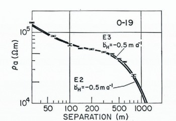
Fig. 11. Plot of apparent resistivity at station O-19. Solid curves are calculated models with parameters c.s shown.
Station O-19 is about 310 km from the ice front, but only 75 km from Mulock Glacier, which is the source of the ice at this site, as shown by the strong radar reflections(Reference BentleyBentley and others, 1979). The ice at this location has thus only a relatively short residence time of perhaps 250 years on the ice shelf (using thedischarge velocity of 290 m year–1 measured for Mulock Glacier (Reference SwithinbankSwithinbank, 1963)), compared with a transient temperature decay constant of some 700 years (calculated from appendix A, equation (2), in Reference WexlerWexler (1960)), so that the assumption of steady-state conditions at O-19 (and at other locations close to outlet glaciers) is probably invalid. Alternatively, because of the proximity of this station to Mulock Glacier, there may be a thin, highly-resistive, basal ice layer similar to that suggested as a possibility at station C-16. In either case, the indicated bottom melt-rate of 0.5 m year–1 could be seriously in error and, in fact, not reflect true melting at all.
Discussion
The resistivity profiles presented here lie in the grid eastern half of the Ross Ice Shelf, at distances between 90 and 400 km from the ice front. At only one, O-19, is there any suggestion of bottom melting, but the lower temperatures that are indicated by the resistivities there more likely occur because the ice has recently been discharged from Mulock Glacier than because of an equilibrium melt condition. Unfortunately, the profiles at Q-13, closest to (about 90 km from) the ice front, are disturbed by local inhomogeneities, nevertheless, the best model fitted to the data, as well as thetemperature measurements to a depth of 100 m, suggests no bottom melting. With an ice movement-rate here of the order of 1 km year–1 (Reference Dorrer, Dorrer, Hofmann and SeufertDorrer and others, 1969), that would mean no measurable average melting over a few hundred kilometers up-stream from Q-13. This is consistent with the estimate of Reference Zumberge and MellorZumberge (1964), based on strain measurements, that the melt-rate decreases from about 1 m year–1 near the ice front to zero at a distance of 80 km from the margin.
Some of the models of Reference Giovinetto and ZumbergeGiovinetto and Zumberge (1968) include bottom freezing-rates of greater than 0.3 m year–1 at distances of 200 km or more from the ice front. Large freezing-rates are not supported by the temperatures measured directly and deduced from resistivides at stations B.C., J-9, O-11, and C-16. Only at M-14 would a large basal freeze-rate be consistent with the observations.
As pointed out above, however, the simple model of resistivity varying only as a function of temperature in the solid ice breaks down if basal freezing occurs over the several hundred years averaging time implied in ![]() , because of the development of a basal zone of relatively much more conductive saline ice. A better approximation in this case is simply to reduce the model ice thickness by the thickness of the basal layer. Model fitting on this basis leads to an estimated basal layer thickness of about 30 m.
, because of the development of a basal zone of relatively much more conductive saline ice. A better approximation in this case is simply to reduce the model ice thickness by the thickness of the basal layer. Model fitting on this basis leads to an estimated basal layer thickness of about 30 m.
Detailed radar profiling on the surface of the ice shelf at M-14 reveals an irregular, patchy reflector about that distance above the base (Fig. 12). Although it is not clear why a fresh-saline ice boundary should be so irregular in geometry and reflectivity, the general agreement between the two lines of evidence suggests such an irregularity strongly.

Fig. 12. An intensity-modulated continuous profile, carried out at M-14 using 35 MHz radar (antenna separation 30 m, attenuation 0 dB). 1 μs in travel time corresponds to about 85 m in ice thickness. The scale of distance along the profile is slightly non-linear. The weak, irregular reflection above the ice-water interface suggests possible saline ice at the bottom of the ice shelf.
The assumption of a basal saline layer is greatly strengthened by maps of airborne-radar reflection characteristics which show M-14 to lie in a poorly-reflecting band (Reference NealNeal, 1979; Reference BentleyBentley and others, 1979). Reference NealNeal (1979) has interpreted this band as arising from basal freezing up-stream of M-14, a conclusion supported with additional evidence by Reference Bentley, Bentley, Clough, Jezek and ShabtaieBentley and others (1979). M-14 is the only resistivity station to lie in one of the poorly-reflecting bands.
Consistent with previous observations at J-9 and B.C. (Reference Bentley, Bentley, Clough, Jezek and ShabtaieBentley, 1979), the measurements continue to suggest an “effective” activation energy in the solid ice closer to 0.15 eV (14 kJ mol–1) than 0.25 eV (24 kJ mol–1).
Acknowledgements
We are especially grateful to L. L. Greischar for his valuable aid with field work at all the stations. Other individuals whose help in field work or in data reduction made this work possible are: D. G. Albert, H. L. Pollak, and P. R. Risse. The authors are indebted to C. C. Langway, Jr, J. H. Cragin, and E. Chiang for furnishing, in advance of publication, the numerical values of the observed temperatures at stations C-16 and Q-13.
Field work and data analysis were supported by National Science Foundation grants OPP72-05805 and DPP76-01415.


