


1. Introduction
Glacier mass balance is important for understanding glacier ice dynamics and estimating the impacts of their changes on local water supplies and global sea levels (Zemp and others, Reference Zemp, Hoelzle and Haeberli2009). Glacierised regions in mid-latitude areas are generally characterised by rough terrain, vast areas and hostile environments. The retrieval of region-wide glacier mass balance via space-borne measurement is efficient, safe and cost-effective compared to in situ measurements. In particular, space-borne geodetic measurements in which differences in the multitemporal glacier surface elevations are multiplied by ice density, can obtain fine resolution results with wide coverage. Therefore, they have become increasingly prevalent for calculating mass balance (Brun and others, Reference Brun, Berthier, Wagnon, Kääb and Désirée2017; Shean and others, Reference Shean2020). Synthetic aperture radar interferometry (InSAR) can work independently of clouds and brightness contrast on ice/snow surfaces and is therefore suitable for obtaining glacier surface elevation. The Shuttle Radar Topography Mission (SRTM), a space-borne InSAR mapping system equipped with C- and X-band microwave sensors, obtained two DEMs on a quasi-global scale from 60° N to 56° S over a span of only 11 d in February 2000 (Farr and others, Reference Farr2007). However, the SRTM was a one-time mission. The German Aerospace Centre launched the TerraSAR-X and TanDEM-X satellites in 2007 and 2010, each carrying an X-band microwave sensor. The two nearly identical satellites fly in close formation, forming the first configurable bistatic synthetic aperture radar (SAR) interferometer that can be used to derive DEMs (Krieger and others, Reference Krieger2007). Precise orbits, high-resolution and seamless coverage make TanDEM-X bistatic images suitable for updating the glacier mass balance over large areas (Groh and others, Reference Groh2014; Rott and others, Reference Rott2014; Dehecq and others, Reference Dehecq2016; Rankl and Braun, Reference Rankl and Braun2016; Li and others, Reference Li2017, Reference Li2018; Neckel and others, Reference Neckel, Loibl and Rankl2017; Lambrecht and others, Reference Lambrecht, Mayer, Wendt, Floricioiu and Völksen2018; Braun and others, Reference Braun2019; Milillo and others, Reference Milillo2019; Seehaus and others, Reference Seehaus2019). However, SAR sensors acquire images with slant-range geometry and the interferometric phase suffers from baseline decorrelation in mountainous areas. When the SAR baseline is constant, the ground-range resolution of the SAR images increases as the local terrain slope approaches the nominal incidence angle, and the correlation between the two SAR signals decreases correspondingly (Zebker and Villasenor, Reference Zebker and Villasenor1992; Lee and Liu, Reference Lee and Liu2001). Furthermore, surface liquid water, which is quite common in the lower reaches of glaciers during the melting season (Shi and others, Reference Shi, Huang, Yao and He2008), can cause surface decorrelation of the interferometric phase (Hoen, Reference Hoen2001). Baseline decorrelation and surface decorrelation of the interferometric phase can lead to bias in InSAR-based elevation measurement. Most importantly, radar signals (i.e. microwaves) can penetrate into snow and ice (Hoen and Zebker, Reference Hoen and Zebker2000; Dall and others, Reference Dall, Madsen, Keller and Forsberg2001; Rignot and others, Reference Rignot, Echelmeyer and Krabill2001; Dall, Reference Dall2007; Gardelle and others, Reference Gardelle, Berthier and Arnaud2012; Neelmeijer and others, Reference Neelmeijer, Motagh and Bookhagen2017) and lead to displacement of the interferometric phase centre. As revealed by in situ radar measurements made in the Antarctic, the phase centre depth of the X-band can reach 4 m in a dry snowpack (Rott and others, Reference Rott, Sturm and Miller1993). In the case of estimating changes in glacier elevation by differencing an InSAR DEM with optical/laser/GNSS (Global Navigation Satellite System) elevation data, the bias (δ) of the InSAR elevation data should therefore be treated carefully.
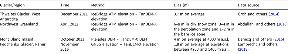
Comparing InSAR-based elevations with optical/laser/GNSS elevations obtained at a similar time provides us with an efficient way of quantifying the bias of InSAR-based elevation (Hoen and Zebker, Reference Hoen and Zebker2000; Dall and others, Reference Dall, Madsen, Keller and Forsberg2001; Rignot and others, Reference Rignot, Echelmeyer and Krabill2001; Berthier and others, Reference Berthier, Arnaud, Vincent and Rémy2006; Groh and others, Reference Groh2014; Dehecq and others, Reference Dehecq2016; Abdullahi and others, Reference Abdullahi2018; Lambrecht and others, Reference Lambrecht, Mayer, Wendt, Floricioiu and Völksen2018) (see Table 1). Groh and others (Reference Groh2014) first measured the bias in the TanDEM-X elevation over glaciers by comparing TanDEM-X DEMs with airborne laser-altimetry elevations that were obtained 1 month ago. Their results indicated an average δ of 3.7 m for the frontal region of the Thwaites Glacier (a large outlet glacier in West Antarctica) in December 2011. Abdullahi and others (Reference Abdullahi2018) measured the bias of TanDEM-X elevations in Northwest Greenland using an analogous method. They found that in April 2012, the values over dry snow, percolation and bare ice zones were 6–8, 3–4 and 1–2 m, respectively. In the mid-latitude glacierised regions, few laser-altimetry elevation datasets that are coincident with TanDEM-X DEMs are available. Dehecq and others (Reference Dehecq2016) therefore measured the bias of TanDEM-X elevations over glaciers in the Mont Blanc massif (Alpine Mountain Range) by differencing a TanDEM-X DEM with a Pléiades DEM (optical) obtained 1 month ago. According to their report, the average δ in October 2013 was 4 m in dry snowpack at 4000 m a.s.l., but was negligible in the zone below 2500 m a.s.l. Lambrecht and others (Reference Lambrecht, Mayer, Wendt, Floricioiu and Völksen2018) compared TanDEM-X DEMs from September and November 2016 with GNSS elevation data from August 2016 and found that the δ for the accumulation zone of the Fedchenko Glacier (Pamir Mountain) was ~1.8 m on average in November, but was negligible in September.
Table 1. Measurements of the bias of TanDEM-X elevations over glaciers
These previous studies presented a basic picture of how the bias of TanDEM-X elevation varies over glacier surfaces. However, the topography and properties of snow/ice (such as grain size, stratification and water content), which directly influence δ, may vary significantly from glacier to glacier. Known as ‘the third pole’, the Tibetan Plateau comprises many high mountains that are controlled by different types of climate. To the best of our knowledge, only Lambrecht and others (Reference Lambrecht, Mayer, Wendt, Floricioiu and Völksen2018) have directly estimated the δ of TanDEM-X elevations over glaciers on the Tibetan Plateau. Therefore, knowledge concerning how the δ of TanDEM-X elevations varies over Tibetan Plateau glaciers is still limited. Previous studies ascribed the measured δ to the X-band penetration depth and did not analyse the other factors that may affecting δ. DEMs that are generated from SPOT-6 stereo images (optical) are often free of problems surrounding signal penetration, surface decorrelation, and baseline correlation over glaciers. In this study, we investigated the X-band δ over two glacierised zones on the Tibetan Plateau by differencing two DEMs that were generated from TanDEM-X and SPOT-6 images. We then quantified the impact that X-band δ has on measurements of the region-wide geodetic mass balance. The results of the DEM differencing had a high resolution and wide coverage, enabling us to reveal the factors that affect the X-band δ. The temporal offsets of the two DEM types in the two regions were only 4 and 6 d, and were much shorter than the temporal offsets in previous studies. The surface condition of glaciers can be reasonably assumed to remain stable over a period of 6 d.
2. Study area
The main ridge of the West Kunlun Mountain Range (79°53′–81°48′ E, 35°06′–35°54′ E) and the Geladandong massif (90°47′–91°16′ E, 33°09′–33°37′ E) in the Dangula Mountain Range are the two most prominent glacial regions on the Tibetan Plateau. The glaciers in these two regions are of big sizes and have clean surfaces. The glacier area on average is 3.4 km2 in the main ridge of the West Kunlun Mountain Range and 3.9 km2 in the Geladandong massif. The Kunlun Mountain Range extends ~2500 km from the Northwest Tibetan Plateau to the Central Tibetan Plateau. Scholars have divided the Kunlun Mountain Range into three sections, namely, the West (75°10′–84°40′ E), Middle (84°40′–95°10′ E) and East (95°10′–103°30′ E) Kunlun Mountain Ranges (Shi and others, Reference Shi, Huang, Yao and He2008). The West Kunlun Mountain Range consists of 16 secondary ranges, of which the main ridge has the largest glacierised area. The glaciers of the main ridge of the West Kunlun Mountain Range are concentrated in three massifs. Our study covered the entire western massif (Fig. 1b). According to the second Chinese Glacier Inventory (CGI-2) (Guo and others, Reference Guo2015), this massif holds 74 glaciers that cover a total area of 173.7 km2 and are distributed over an altitude range of 5100–6500 m. The West Kunlun Mountain Range is influenced by the westerly winds and a climate characterised as extremely cold and dry. The annual average temperature and precipitation near the snowline (at ~5900 m a.s.l.) are ~−14°C and 300 mm, respectively (Zhang and others, Reference Zhang, An, Yang and Jiao1989). Most of the annual precipitation occurs between May and September, and the northern slope receives more precipitation compared to the southern slope (Zhang and others, Reference Zhang, An, Yang and Jiao1989). An ice temperature of −19.6°C was previously measured at a depth of 4 m in a glacier on the southern slope, which is very close to the temperature of the ice measured in the Antarctic Peninsula and South Greenland (Shi and others, Reference Shi, Huang, Yao and He2008).
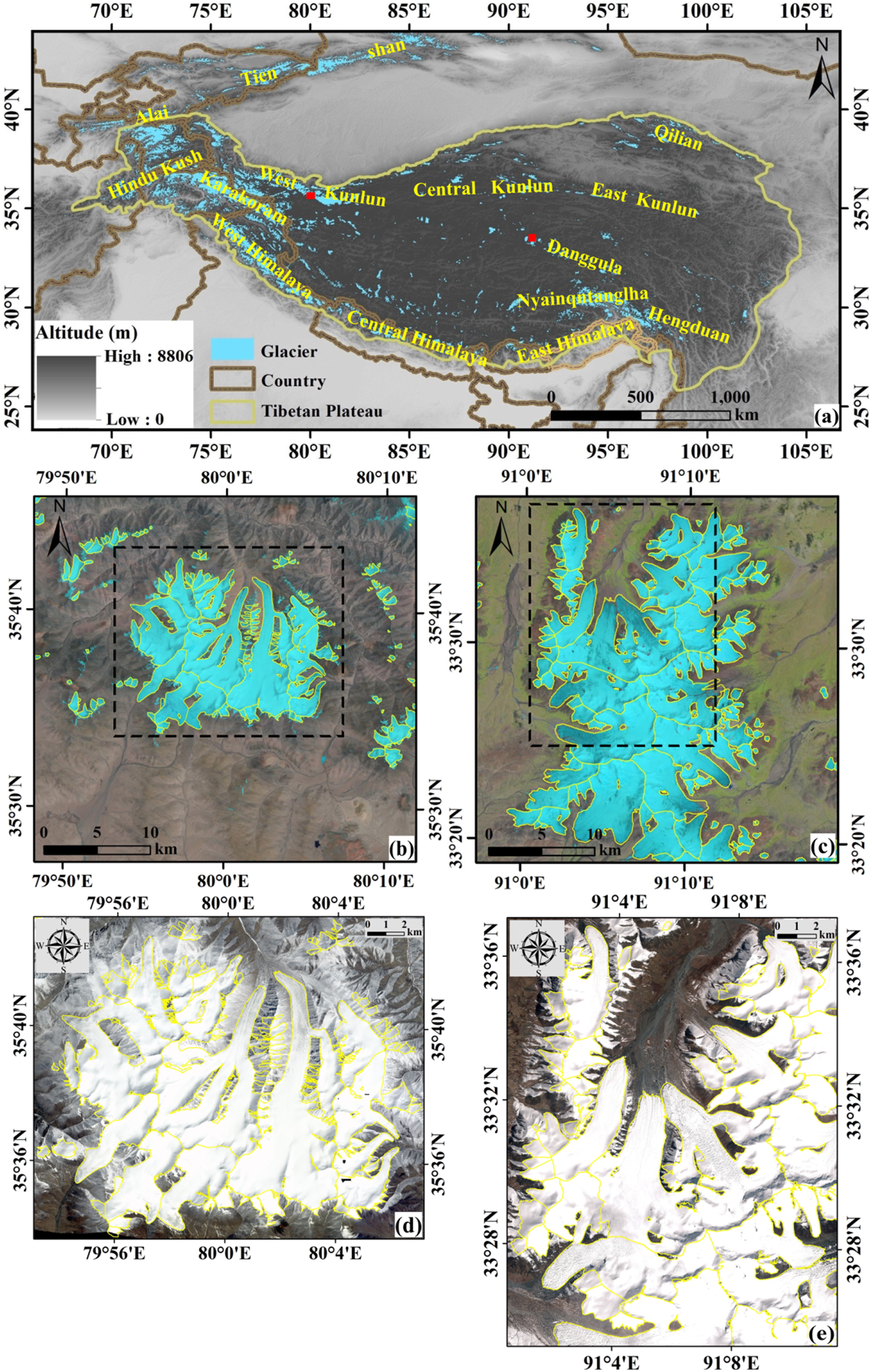
Fig. 1. (a) Topography and glacier distribution on the Tibetan Plateau. The main glacierised mountain ranges in and surrounding the Tibetan Plateau are denoted with yellow text. The background is a 3 arc-second SRTM C-band DEM. Red rectangles denote the locations of the areas shown in (b) and (c). (b) Landsat-8 image (RGB bands: 432, 14 July 2018) showing part of the main ridge in the West Kunlun Mountain Range. (c) Landsat-8 image (RGB bands: 432, 25 July 2019) showing part of the Geladandong massif in the Dangula Mountain Range. Rectangles of black dashes in (b) and (c) denote areas where the SPOT-6 and TanDEM-X images overlap, i.e. our study areas. The yellow glacier outlines in (b) and (c) were acquired from the second Chinese Glacier Inventory. (d) SPOT-6 image (RGB bands: 123, 10 April 2014) at site 1. (e) SPOT-6 image (RGB bands: 123, 6 October 2013) at site 2. The yellow glacier outlines in (d) and (e) are updated based on the SPOT-6 images.
The second study area is located in the Geladandong massif, which belongs to the Dangula Mountain Range that extends ~1000 km in the hinterland of the Tibetan Plateau. With 40 snow peaks over 6000 m a.s.l., the Geladandong massif is the most densely glacierised region of the Dangula Mountain Range, and serves as the headwaters of the Yangtze River, which is the longest river in China. The glacierised region extends ~50 and 25 km in northsouth and eastwest directions, respectively. According to the CGI-2, this region includes 119 glaciers that cover a total area of 609.8 km2 and are distributed over an altitude range of 5200–6600 m. The snowline in this region is ~5650 m a.s.l. Our study covers the northern part of the glacierised region (Fig. 1c). The Geladandong massif is influenced by continental air masses and its climate is extremely cold and dry. The annual average temperature and precipitation at the foot of the Geladandong massif are ~−5°C and 200 mm, respectively (Wang and others, Reference Wang, Wu, Xu and Liu2013). According to the meteorological data collected at Anduo Station (4800 m a.s.l., close to the Geladandong massif), most of the annual precipitation occurs between May and September when the monthly average temperature is above freezing (Ye and others, Reference Ye, Kang, Chen and Wang2006). Ascending from 5000 m a.s.l., the amount of precipitation increases because of the strong local circulation (up to 500 mm) (Wang and others, Reference Wang, Wu, Xu and Liu2013). For simplification, the study sites in the West Kunlun Mountain Range and Geladandong massif are referred to as site 1 and site 2, respectively, in the following text, tables and figures.
3. Data
3.1. TanDEM-X imagery
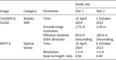
The TerraSAR-X and TanDEM-X satellites form a new generation of SAR constellations that can work in three cooperative modes: bistatic, pursuit monostatic and alternating bistatic. When the bistatic mode is used, either the TanDEM-X or TerraSAR-X satellite sends out a radar signal and the scattered echo is then recorded by the two satellites simultaneously. Therefore, the bistatic TanDEM-X image pair is not affected by temporal decorrelation or atmospheric variation. TerraSAR-X can perform imaging in three modes: stripmap, scanSAR and spotlight. Characterised by a good balance between swath width and resolution, bistatic stripmap images were adopted to produce the global TanDEM-X DEM (Rizzoli and others, Reference Rizzoli2017a). Note that the released TanDEM-X images are referred to as co-registered single-look slant-range complex (CoSSC) images that have been prepared for interferometric processing. In this study, two single-polarimetric stripmap bistatic CoSSC images that were acquired on 16 April 2014 and 2 October 2013 were obtained from the German Aerospace Center to generate X-band DEMs. The stripmap of the TanDEM-X image generally has a swath of ~30 km × 50 km. Table 2 provides details of the bistatic TanDEM-X CoSSC images.
Table 2. TanDEM-X and SPOT-6 images used in this study
3.2. SPOT-6 imagery
SPOT-6 is an optical satellite that was launched by the European Aeronautic Defence and Space Agency in 2012. It provides a good balance between high resolution and wide coverage. The standard image swath width of SPOT-6 is 60 km, and the resolutions of the along-track stereo panchromatic images and nadir multispectral (blue, green, red and near-infrared) images are 1.5 and 6 m, respectively. The number of along-track stereo looking directions is three (triple stereo). As with Pléiades panchromatic imagery, SPOT-6 panchromatic imagery is coded with 12-bit resolution. Compared to the 8-bit encoding used by SPOT-5, PRISM and ASTER, 12-bit encoding reduces the risk of pixel saturation over zones that lack texture, such as glacier firn basins. The image contrast over ice and snow is correspondingly enhanced (Berthier and others, Reference Berthier2014). Without ground control points (GCPs), a SPOT-6 image can be located with an accuracy of 10 m (90% circular error) if a reference 3-D DEM is available (Grazzini and Astrand, Reference Grazzini and Astrand2013). In this study, two back–front looking stereo SPOT-6 images acquired on 10 April 2014 and 6 October 2013 were obtained from the SPOT Image Company to generate new optical DEMs and update the glacier boundaries. Table 2 and Figure 1 provide details of the SPOT-6 images used in this study.
3.3. SRTM DEM
One arc-second C-band SRTM DEM (NASADEM_HGTv001) was obtained from the Land Processes Distributed Active Archive Centre (https://lpdaac.usgs.gov/) to assist in the generation of new TanDEM-X DEMs. NASADEM_HGTv001 was derived from original SRTM interferometric data, and its quality was improved using the Terra Advanced Spaceborne Thermal and Reflection Radiometer (ASTER) Global DEM, Advanced Land Observing Satellite Panchromatic Remote-sensing instrument for Stereo Mapping (PRISM) AW3D30 DEM, and Ice, Cloud and Land Elevation Satellite (ICESat) Geoscience Laser Altimeter System (GLAS) GCPs. The data voids were filled through interpolation (https://lpdaac.usgs.gov/products/nasadem_hgtv001/).
4. Methods
4.1. Generation of TanDEM-X DEMs
The differential InSAR (D-InSAR) suite of the GAMMA Remote-Sensing Software 2018 was used to generate DEMs from the TanDEM-X/CoSSC images. The basic D-InSAR processing for DEMs involves multi-looking of SAR images, generation of interferograms, forward geocoding of an external DEM (from map to SAR coordinates), simulation of topographic phases, subtraction of topographic phases, filtering of differential interferograms, unwrapping of differential phases, retrieval of differential heights and backward geocoding of a new DEM (from SAR to map coordinates) (Li and others, Reference Li2017). The fringe density of the interferogram of a short microwave is significant for high mountains, rendering the interferometric phase difficult to unwrap. To address this problem, we simulated a topographic phase from the geocoded 1 arc-second SRTM C-band DEM and subtracted it from the original interferogram. Unwrapping a differential interferometric phase with sparse fringes is relatively easy (Seehaus and others, Reference Seehaus2016; Guo and others, Reference Guo2020a). Subsequently, a reference point (assumed to be the zero phase) was manually set on a stable surface. As the noise level was low in this study, the minimum cost flow method was adopted to unwrap the differential phase (Werner and others, Reference Werner, Wegmüller and Strozzi2002). A new DEM was then obtained by adding the SRTM DEM to the differential height retrieved from the unwrapped differential phase. The resolution of the SRTM C-band DEM is much lower than that of the TanDEM-X CoSSC imagery. We then used the newly generated DEM as the external DEM and implemented the D-InSAR procedure iteratively to achieve a high-resolution DEM (Du and others, Reference Du, Feng, Li, Zhu and Peng2015). As mentioned previously, before simulating the topographic phase from the external DEM, we needed to forward geocode the external DEM. The core step of forward geocoding is to simulate a SAR image from the external DEM and co-register it with a real SAR image. When the real SAR image is much finer than the simulated SAR image, the SAR image needs to be multi-looked in order to facilitate the co-registration process. The resolution of the output of backward geocoding (TanDEM-X DEM in this study) is subject to the resolution of the external DEM. To improve the resolution of the output TanDEM-X DEM, we can oversample the external DEM. However, the oversampling factor cannot be too high; otherwise, the simulated SAR image will be too coarse, and the co-registration will be unreliable. In this study, the external DEM was oversampled by a factor of 2 × 2 during the subsequent iterative process. The factors of the TanDEM-X multi-looking were then reduced gradually as iteration continued until a DEM with the desired resolution was achieved. Finally, we generated TanDEM-X DEMs with a resolution of 4 m. The flowchart of generating TanDEM-X DEMs with high resolution is presented in Figure 2.
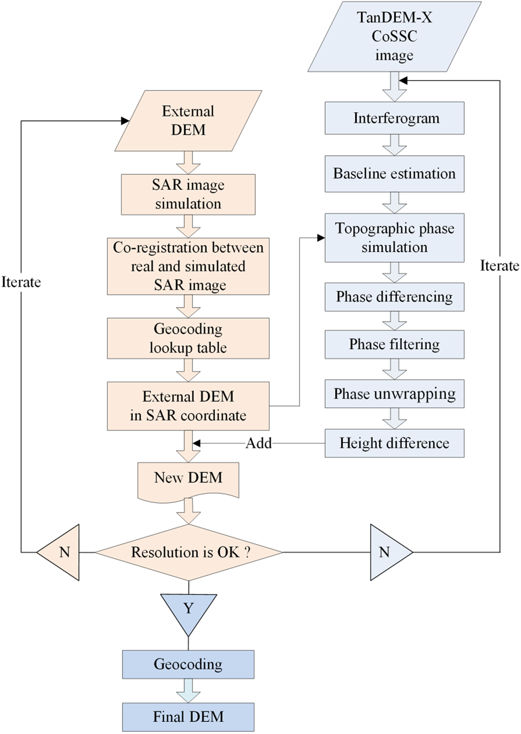
Fig. 2. Procedure of generating a new TanDEM-X DEM.
4.2. Generation of SPOT-6 DEMs
The Satellite Ortho Suite in PCI Geomatica 2017 software was used to generate DEMs from the SPOT-6 stereo images. The exterior (absolute) orientation was performed using the traditional method, i.e. a space resection, which is based on GCPs and a collinearity equation. The two glacial sites are located in remote depopulated zones. As the terrain is rough and the climatic conditions are hostile, accessing the two glacial centres and establishing field survey-based GCPs would be quite difficult. Previous studies (Pieczonka and others, Reference Pieczonka, Bolch, Wei and Liu2013; Holzer and others, Reference Holzer2015; Li and others, Reference Li2018) have proved that the combination of an SRTM-C DEM and orthorectified Landsat images (panchromatic/multispectral fused) can be used as an alternative GCP source for glacial DEM extraction. The elevations of all the chosen GCPs were cross-checked in Google Earth™ (Holzer and others, Reference Holzer2015). In total, 17 and 15 GCPs were used for sites 1 and 2, respectively. The residual errors of the GCP bundle adjustment were ~1.5 m. Approximately 50 evenly distributed tie points were collected for the interior (relative) orientation of each image. In choosing the tie points, ground features such as rocks, river confluences, ice crevasses, lakes and horns were preferred. After the GCPs and tie points were collected, stereo image orientation, quasi-epipolar image creation, image registration, DEM generation and image orthorectification processes were conducted in sequence. The output SPOT-6 DEMs have a resolution of 4 m. PCI Geomatica 2017 offers a score map for evaluating the reliability of a generated DEM. The scores of adjacent pixels should theoretically be different because the spectral characteristics of adjacent pixels are inhomogeneous. By differencing the newly generated SPOT-6 DEM with other DEMs, we found that the SPOT-6 elevations in the area with even scores were basically outliers, regardless of how high the scores were. Therefore, we masked the SPOT elevations in the areas with homogeneous scores (Holzer and others, Reference Holzer2015; Li and others, Reference Li2018). Finally, low-strength median filtering was applied to reduce the outliers (Guo and others, Reference Guo2020b).
4.3. Estimation of the bias of the TanDEM-X elevations
The bias (δ) of TanDEM-X elevations over glaciers was estimated by subtracting the TanDEM-X DEM from the SPOT-6 DEM. As mentioned above, over glacier surface SPOT-6 images do not suffer from problems associated with signal penetration and phase decorrelation. However, before differencing the two DEMs, it is necessary to prove the reliability of SPOT-6 DEM. The ICESat-2/ATLAS ATL06 L3A land ice height product (version 2), which is well-known for its accuracy, was used to evaluate the SPOT-6 DEM. Only ATL06 points in non-glacierised regions were chosen for evaluation because the acquisition time of the ICESat-2 data are 5 years later than that of the SPOT-6 images. The along-track resolution of the ATL06 product is 20 m. A total of 1061 ATL06 points acquired on 15 April 2019 were used for the West Kunlun study area and 1797 points acquired on 27 October 2018 for the Dangdula study area. The SPOT-6 elevation at the ATL06 point was extracted by bilinear interpolation. Relative to the ATL06 elevations, the SPOT-6 DEMs generated in the West Kunlun and Dangula study areas had root mean square errors (RMSEs) of 2.3 and 3.7 m, respectively. Small RMSEs indicate that the SPOT-6 DEMs are of good accuracy.
The DEMs were then co-registered before differencing. Although the TanDEM-X and SPOT-6 DEMs share the same vertical and horizontal data, the geolocation accuracies and systematic errors might be inconsistent because they were obtained via different sensors and methods. As shown in Figure 3a, significant positive and negative elevation differences can be found along the hill ridges, indicating horizontal shifts between the SPOT-6 and TanDEM-X DEMs. The analytical DEM co-registration method presented by Nuth and Kääb (Reference Nuth and Kääb2011) was used in this study. The DEM shift parameters can be estimated from the relationship between the terrain parameters (slope and aspect) and the raw elevation differences over stable areas (Fig. 4a). Vegetation cover is rare in the study area and the ice-free areas were deemed stable because of the absence of landslides and water bodies in the area. To mask the glacier areas precisely, we manually updated the glacier outlines from CGI-2 based on the orthorectified SPOT-6 images. SPOT-6 DEMs are not subject to microwave penetration or interferometric decorrelation and were therefore used as reference DEMs in the current study. The TanDEM-X DEMs were shifted according to the parameters derived through analytical co-registration. Data gaps in the elevation difference map mainly originate from the baseline decorrelation of the interferometric phase, SAR image shadow and the low contrast of the SPOT-6 images.
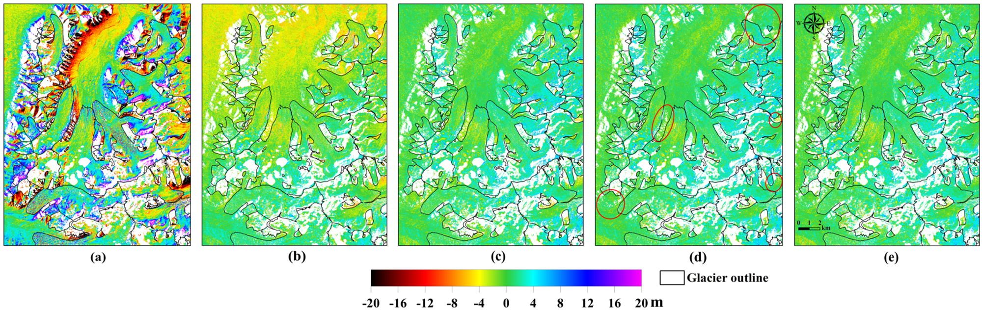
Fig. 3. Improvement to the elevation difference map of site 2 (SPOT-6 DEM on 6/10/2013 minus the TanDEM-X DEM on 2/10/2013). (a) Raw elevation difference map. (b) Elevation difference map after DEM co-registration. (c) Elevation difference map after planimetric position-related bias correction. (d) Elevation difference map after the second round of DEM co-registration. (e) Elevation difference map after terrain curvature-related bias correction. White areas represent gaps in the elevation difference maps. The red ellipses in (d) mark non-glacierised areas with bias correction. The location of the study area shown here is marked by the black dashed rectangle in Fig. 1c.
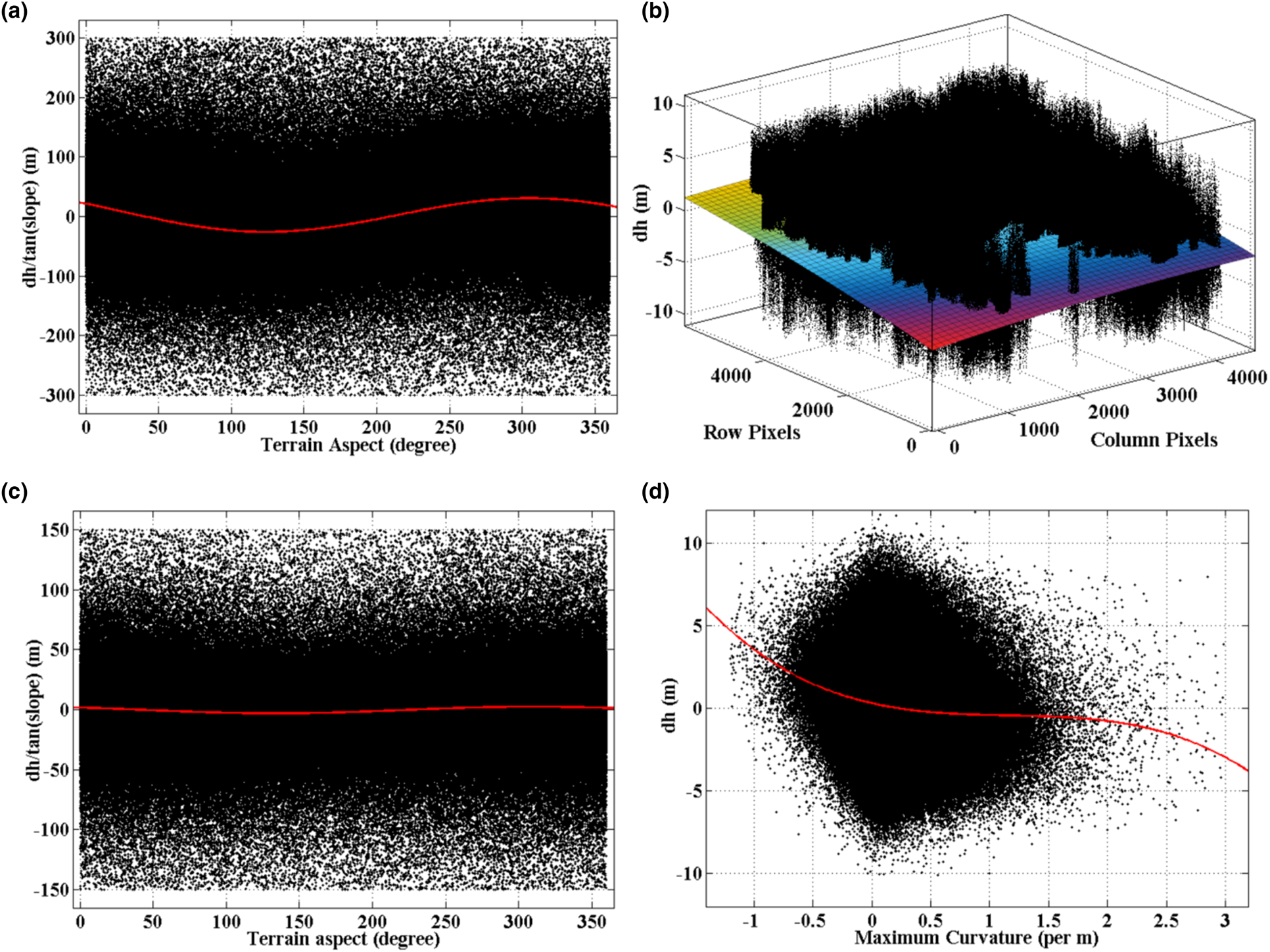
Fig. 4. Universal bias trends fitted for the elevation differences over stable areas in site 2. (a) Scatter plot between the ratio of the raw elevation difference over the tangent of the slope [dh/tan(slope)] and the terrain aspect. The red curve is the fitted model (cosine function). (b) Three-dimensional view of the scatter plot of the elevation difference (after the first round of DEM co-registration) vs the planimetric position. The surface is the fitted trend obtained using a quadratic polynomial. (c) Scatter plot between the ratio in the elevation difference (after the first round of DEM co-registration and correction of planimetric error) to the tangent of the slope [dh/tan(slope)] and the terrain aspect. The red curve is the fitted model (cosine function). (d) Scatter plot of the elevation difference (after two rounds of DEM co-registration and correction of planimetric error) vs the terrain maximum curvature. The red curve is the fitted trend obtained using a third-order polynomial.
After the DEM co-registration and differencing, we successively examined the systematic bias in the elevation difference map. Following the processing conducted in previous studies, we examined and corrected the systematic bias by fitting a trend from the nonglacial samples and removing it from the elevation difference map, based on the hypothesis that the bias over glacial and stable regions is homogeneous (Nuth and Kääb, Reference Nuth and Kääb2011). Our experiments confirmed that this type of processing is simple but effective. Only the elevation difference maps for site 2 are used to illustrate the effects as the experiments conducted over the two study sites were similar (those for site 1 can be found in the Supplementary material). As shown in Figure 3b, a northsouth tilted systematic bias exists in the elevation difference map. A similar bias was also found by , Dehecq and others (Reference Dehecq2016) and Li and others (Reference Li2017, Reference Li2018). The InSAR residual baseline and inaccuracy of the selected GCPs can induce planimetric bias in the final DEM. As this bias is clearly correlated with the planimetric position, we fitted it as a universal trend using the quadratic surface polynomial model (Fig. 4b), and then removed the bias from the elevation difference map. Figure 3c indicates that the elevation differences over the stable regions decrease markedly and those over the glaciers become increasingly uniform after planimetric-related bias correction. However, obvious systematic bias can still be discerned on some of the non-glacierised slopes. We checked the relationship between the terrain parameters (slope and aspect) and the elevation differences over stable areas (Fig. 4c) and found those bias could be removed by performing the analytical DEM co-registration again. It is likely that the obvious planimetric-related bias affected the estimation of the DEM shifting parameters at the start of the process because the planimetric-related bias was inconspicuous at site 1, and there was no need for the analytical DEM co-registration to be carried out again (Fig. S1 in the Supplementary material). Figure 3d shows that the elevation differences over the stable regions become smaller after the second round of analytical DEM co-registration. We also found a slight curvature-related bias in the elevation difference map, which may originate from the small difference between the resolution of the TanDEM-X/CoSSC image and the SPOT-6 image (Paul, Reference Paul2008; Gardelle and others, Reference Gardelle, Berthier and Arnaud2012). The bias was fitted as a universal bias trend using a third-order polynomial (see Fig. 4d) and was then removed from the elevation difference map. The visual improvement in the elevation difference map was minor following this correction (Fig. 3e); however, the median and mean of the elevation differences over the stable regions decreased (Table 3).
Table 3. Statistics of the elevation differences over stable areas in Figure 4
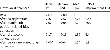
a The computed value before rounding is 0.0003.
As the elevation differences over stable areas are supposed to be zero, the normalised median absolute deviation (NMAD) and the median and mean of the elevation differences over stable areas are used to quantify the effects of the bias correction. The standard deviation (std dev.) of a sample set is known to be capable of scaling the dispersion of individual data points from the mean. When the mean of the elevation differences is close to zero, the std dev. can be considered as a direct indicator of accuracy. However, the common approach to std dev. computation is prone to influence from outliers. According to Höhle and Höhle (Reference Höhle and Höhle2009) and Pieczonka and others (Reference Pieczonka, Bolch, Wei and Liu2013), the NMAD is less sensitive to outliers and is a robust estimator of std dev.. The formula used for NMAD computation is:
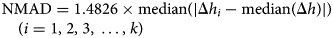
where Δh is the observed elevation difference observation and k is the number of observations. Table 3 shows that after DEM co-registration and bias correction, the NMAD, median and mean of the nonglacial elevation difference all decrease considerably. The parameter changes and the visual changes to the elevation difference maps (Fig. 3) confirm that our correction of the systematic bias in the elevation difference maps is necessary and useful.
The average δ was computed using the hypsometric method, i.e. dividing the glacial altitude range into N bands and computing the average δ over the glacier surface within each altitude band, and then deriving the area-weighted average (Kääb, Reference Kääb2008). The void areas were assumed to have the average δ of the altitude band to which they belong (McNabb and others, Reference Mcnabb, Nuth, Kääb and Girod2019). To present the distribution of δ at a fine scale, an altitude band of 10 m was used.
4.4. Delineation of the glacier firn line
To facilitate the interpretation of the factors that impact δ, we delineated the transient glacier firn line from the orthorectified SAR backscatter coefficient map. The X-band backscatter coefficient is sensitive to surface wetness (Rott and Mätzler, Reference Rott and Mätzler1987). In April or October in the northern hemisphere, the surface wetness of the ablation zone is higher than that of the wet snow zone. Hence, the backscatter coefficient of the wet snow zone is higher than that of the ablation zone (Fig. 5), which enables us to manually delineate the demarcation line between these two zones, which is known as the firn line (Adam and others, Reference Adam, Pietroniro and Brugman1997; König and others, Reference König, Winther, Knudsen and Guneriussen2001a; Huang and others, Reference Huang, Li, Tian, Chen and Zhou2013). Note that during the period from July to September, the backscatter coefficient of the wet snow zone clearly becomes lower than that of the ablation zone because both zones have high surface water content; however, the ablation zone has a rougher surface (Huang and others, Reference Huang, Li, Tian, Chen and Zhou2013). We avoided the hillsides for delineation of the firn line because the backscatter coefficient over the fore and back slopes is usually overestimated and underestimated, respectively. Also, the backscatter coefficient within areas with slopes higher than 30° was masked. The glaciers that were used in delineating the firn line were sampled evenly with regards to size and orientation. At site 1 (West Kunlun), 13 glaciers were sampled, and their area accounted for 88.8% of the entire glacier area (according to the modified CGI-2). At site 2 (Geladandong), 16 glaciers were sampled, and their area accounted for 74.1% of the entire glacier area (according to the modified CGI-2). The representative firn line was computed for each study site through an area-weighted average.
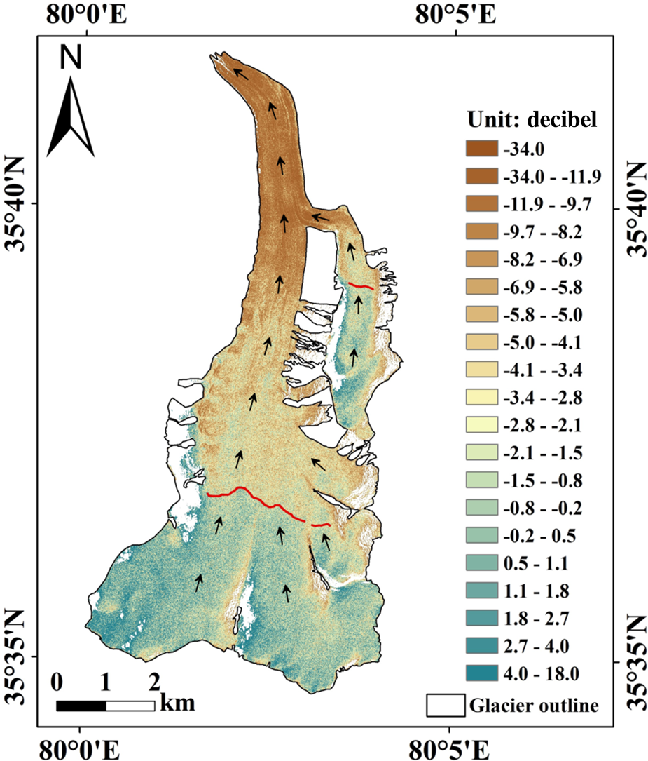
Fig. 5. Backscatter coefficient of the TanDEM-X image for the largest glacier in site 1 on 16 April 2014 (CGI-2 ID: 5Y641J0199). Red lines are manually delineated glacier firn line and black arrows denote the approximate ice flow directions. The white areas within the glacier outline denote gaps in the data.
4.5. Uncertainty analysis
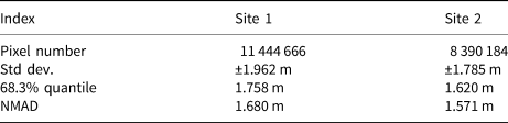
In this study, the absolute accuracy of the DEMs was inferior to the relative accuracy because the former denotes the control of DEMs in association with a particular datum, while the latter indicates the uncertainty of the elevation differences (Cox and March, Reference Cox and March2004). As a result of the paucity of synchronous highly precise measurements, observations over the stable regions were used to scale the uncertainty of the results. The std dev., NMAD and 68.3% quantile of the elevation difference observations (SPOT-6 DEM minus TanDEM-X DEM) over the stable regions were computed (Table 4). The 68.3% quantile reflects the data range in which 68.3% of the absolute elevation difference observations are located. In the case of a normal distribution, the 68.3% quantile, NMAD and std dev. of the samples should all be close. In this study, the 68.3% quantile and NMAD differed slightly from the std dev., indicating a slightly non-normal distribution for the elevation difference observations over the stable regions. Referring to Pieczonka and others (Reference Pieczonka, Bolch, Wei and Liu2013), we used the NMAD to evaluate the uncertainty of the elevation difference at the individual pixel scale, i.e. ±1.680 and ±1.571 m for sites 1 and 2, respectively.
Table 4. Statistics of the elevation difference observations over the stable regions
However, the result achieved is the average elevation difference, and the spatial autocorrelation of the elevation difference should be taken into account. According to Rolstad and others (Reference Rolstad, Haug and Denby2009), the uncertainty of the average elevation difference over glaciers (ζ average) can be estimated using the following formula:
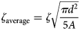
where ζ is the uncertainty of the elevation difference at the individual pixel scale (i.e. the NMAD of the elevation difference over stable regions), A is the observed glacier area and d is the auto-correlation length of the elevation difference over stable regions that can be derived by fitting a spherical semivariogram model to an empirical semivariogram of the samples (Rolstad and others, Reference Rolstad, Haug and Denby2009), which can be achieved using the Geostatistical Analyst tool in ArcGIS software. The values of d derived in sites 1 and 2 are 95 and 109 m, respectively. The region-wide ζ average calculated over study sites 1 and 2 are ±0.012 and ±0.011 m, respectively. Our measurement benefits from the high-resolution and high number of observations in our DEM differences, thus yielding relatively small region-wide uncertainties. However, we did not assess any errors that might originate from the short time difference between acquisition (<6 d) and assumed that the systematic bias of DEMs was negligible after alignment and correction of the DEM was carried out.
5. Results
A total of 7 483 097 and 10 259 605 effective observations of glacial δ were obtained in sites 1 and 2, respectively. Figure 6 displays the values of δ for the two study sites. The average δ over the stable areas in sites 1 and 2 are 0.3 and −4.0 mm, respectively. Except for a few slopes (such as region A in Fig. 6a) and fresh snow packs (such as region B in Fig. 6b), most of the non-glacierised regions have a value of δ that is close to zero, indicating that the TanDEM-X and SPOT-6 DEMs are in good agreement. Fresh snow packs are known to have favourable conditions for microwave penetration. TanDEM-X elevation refers to the elevation of the bedrock below the snow, while SPOT-6 elevation refers to the surface elevation of fresh snow packs. The reason for the δ on ice-free slopes is given in Section 6.1. In site 1, the average δ over the glaciers with an area of 175.0 km2 is 2.106 ± 0.012 m, and in site 2, the average δ over the glaciers with an area of 228.8 km2 is 1.523 ± 0.011 m. In general, the InSAR DEMs extracted from the TanDEM-X images are underestimated by ~2 m in the studied glacier areas. Figure 7 displays the area covered by glaciers and the average δ for each altitude band (10 m). The April glacier firn line measured at the West Kunlun Mountain Ranges is 5928 m, and the October firn line measured at the Dangula Mountain Ranges is 5731 m. In site 1, the average δ above and below the firn line are 2.612 ± 0.019 and 1.425 ± 0.016 m, respectively. In site 2, the corresponding values are 1.942 ± 0.020 and 0.986 ± 0.014 m, respectively. The number of δ between 1 and 5 m in the West Kunlun glacier area takes up a higher proportion than that in the Dangula glacier area (61.9% compared to 48.7%). Some δ observed in the firn basin reach up to 7 m (at 5970 m a.s.l.). Excluding the small surrounding glaciers in site 1 (distributed below 5400 m a.s.l.), the general variation patterns of the δ in the two study sites are similar. In the glacier areas above the firn line, δ generally increases with altitude; and below the firn line, δ first decreases and then increases with altitude. Prominent values of δ are observed not only in the high firn basins, but also in the lower tongues (see glaciers 1–5 in Fig. 6a).
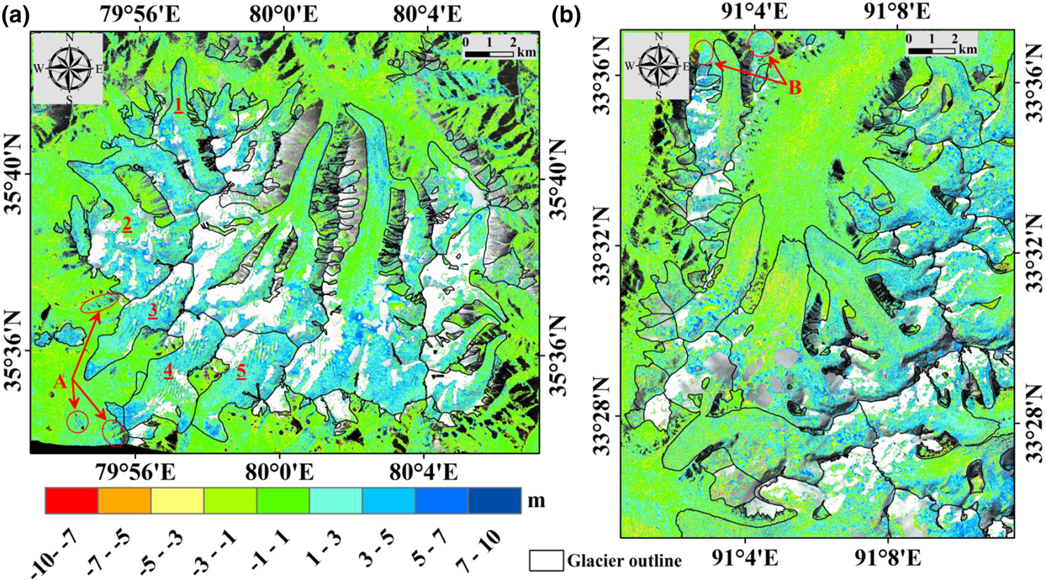
Fig. 6. Observed bias of the TanDEM-X DEMs for site 1 (a) and site 2 (b). Backgrounds are presented by SPOT-6 images (RGB: bands 123) acquired on 10 April 2014 (a) and 6 October 2013 (b). The areas where the background image can be seen are gaps in the data. Numbers 1–5 mark the glaciers mentioned in the text. Regions A and B (within the red ellipses) denote the non-glacierised slopes and fresh snow packs mentioned in Section 5, respectively.
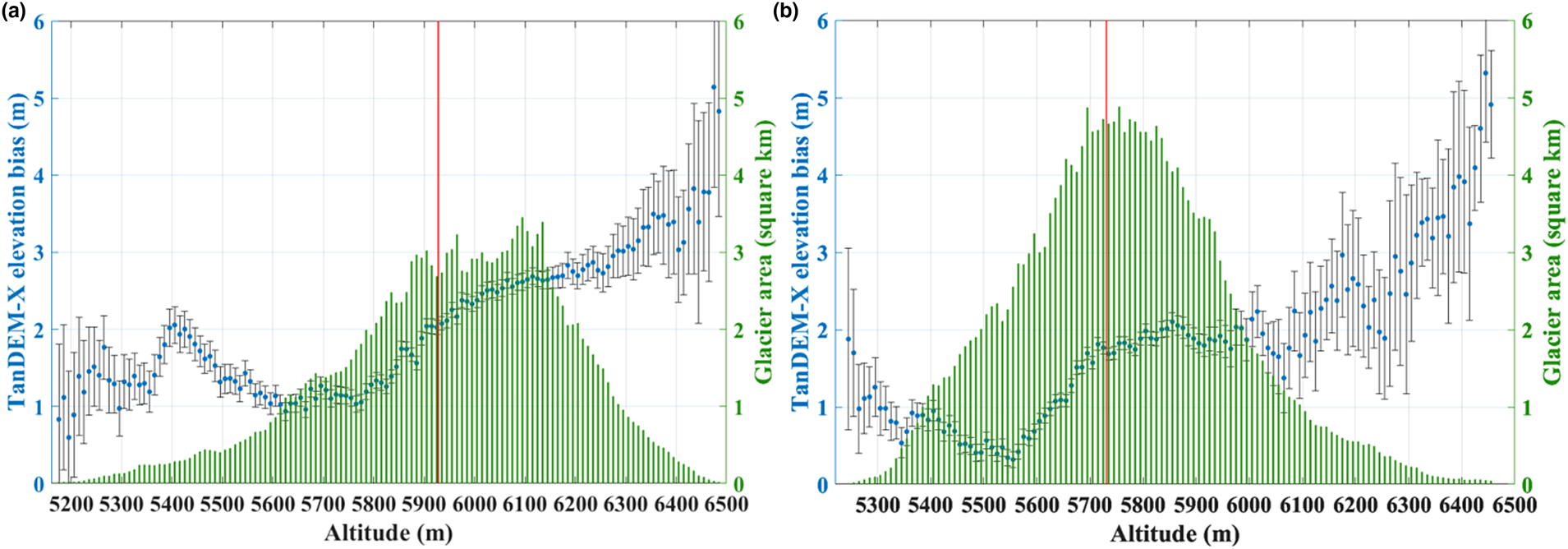
Fig. 7. Glacier area and average TanDEM-X elevation bias (error bar: 1 std dev.) for every 10-m altitude band. (a) Site 1. (b) Site 2. The red lines denote the altitudes of the average firn lines.
6. Discussion
6.1. Main factors of TanDEM-X elevation bias over glaciers
In theory, the instrumental errors of the TanDEM-X satellite (including the platform positioning error, baseline error and slant-range error) have been well controlled, and the observed δ is mainly caused by interferometric phase errors. As mentioned previously, the bistatic TanDEM-X image pairs are not affected by temporal decorrelation or atmospheric variation (Krieger and others, Reference Krieger2007). The interferometric phase error is mainly caused by microwave penetration (displacement of the phase centre), surface decorrelation and baseline decorrelation. The capability of microwaves to penetrate the surfaces of glaciers is closely correlated with the water content, layer stratification, grain size and mass density of a glacier (Rott and others, Reference Rott, Sturm and Miller1993; Hoen and Zebker, Reference Hoen and Zebker2000; Rizzoli and others, Reference Rizzoli, Martone, Rott and Moreira2017b; Lambrecht and others, Reference Lambrecht, Mayer, Wendt, Floricioiu and Völksen2018). Technically, from head to terminus, a glacier can be divided into four zones according to its physical properties, i.e. the dry snow zone, percolation zone, wet snow zone and ablation zone (Cuffey and Paterson, Reference Cuffey and Paterson2010). The first three zones comprise the accumulation zone. The mass density, mass heterogeneity, grain size and water content generally decrease from the ablation zone to the dry snow zone. However, glaciers with four zones are mainly distributed in the Arctic and Antarctic regions (König and others, Reference König, Winther and Isaksson2001b). Based on a large number of field investigations, glaciologists have found that most glaciers in High Asia (including the Altay, Kunlun, Qilian, Himalaya and Hengduan Mountain Ranges) do not have dry snow zones, except for those in the extremely high regions of the Karakoram Mountain Ranges, Tianshan Mountain Ranges and Eastern Pamir (Shi and others, Reference Shi, Huang, Yao and He2008; Hewitt, Reference Hewitt2014). Hence, the accumulation zones of the glaciers in our study areas consist of percolation and wet snow zones. Low water content, simple stratification, small grain size and low mass density generally correspond to deep microwave penetration. Ascending from the firn line to the glacier head, the microwave penetration depth should gradually increase (for debris-free glaciers). As shown in Figure 7, the δ above the firn line increases with altitude. Meanwhile, as suggested by Figures 8 and 9, between 6070 and 6350 m a.s.l., the backscatter coefficient and interferometric coherence of the TanDEM-X bistatic image decrease while δ increases. This observation coincides with previous findings, in that deep penetration over glacier dry snow zones and percolation zones can cause significant volume decorrelation and the loss of signal (Rott and others, Reference Rott, Sturm and Miller1993; Hoen and Zebker, Reference Hoen and Zebker2000; Martone and others, Reference Martone, Rizzoli and Krieger2016; Rizzoli and others, Reference Rizzoli, Martone, Rott and Moreira2017b; Abdullahi and others, Reference Abdullahi2018). In the wet snow zone, the incident microwaves can interact with internal ice structures such as ice pipes and lenses that have the similar length as the microwave (Rizzoli and others, Reference Rizzoli, Martone, Rott and Moreira2017b). The diffuse and specular reflections at the boundaries of internal ice structures can contribute considerable amounts of power to radar echoes (Rott and others, Reference Rott, Sturm and Miller1993; Jezek and others, Reference Jezek, Gogineni and Shanableh1994). This characteristic may, in fact, explain why the SAR backscatter coefficient and interferometric coherence between 5960 (the altitude of the firn line) and 6070 m a.s.l. are relatively high, even though the penetration is considerable (Fig. 9). In general, the δ observed above the firn line is mainly caused by microwave penetration. Note that glaciers of different size and altitude have hypsometric differences and different surface physical properties (Fig. 8). In Figure 9, we chose glaciers 1–5 of site 1 for illustrative purposes because they have prominent δ and similar altitude ranges.
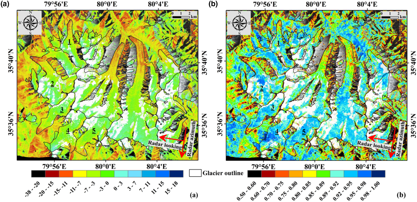
Fig. 8. Backscatter coefficients (unit: decibel) (a) and interferometric coherence (b) of the TanDEM-X bistatic image (16 April 2014) in site 1. Background is presented by a SPOT-6 image (RGB: bands 123, 10 April 2014). The radar flying and looking directions are denoted by the red arrows. The areas where the background can be seen are gaps in the data. Numbers 1–5 mark the glaciers mentioned in the text.
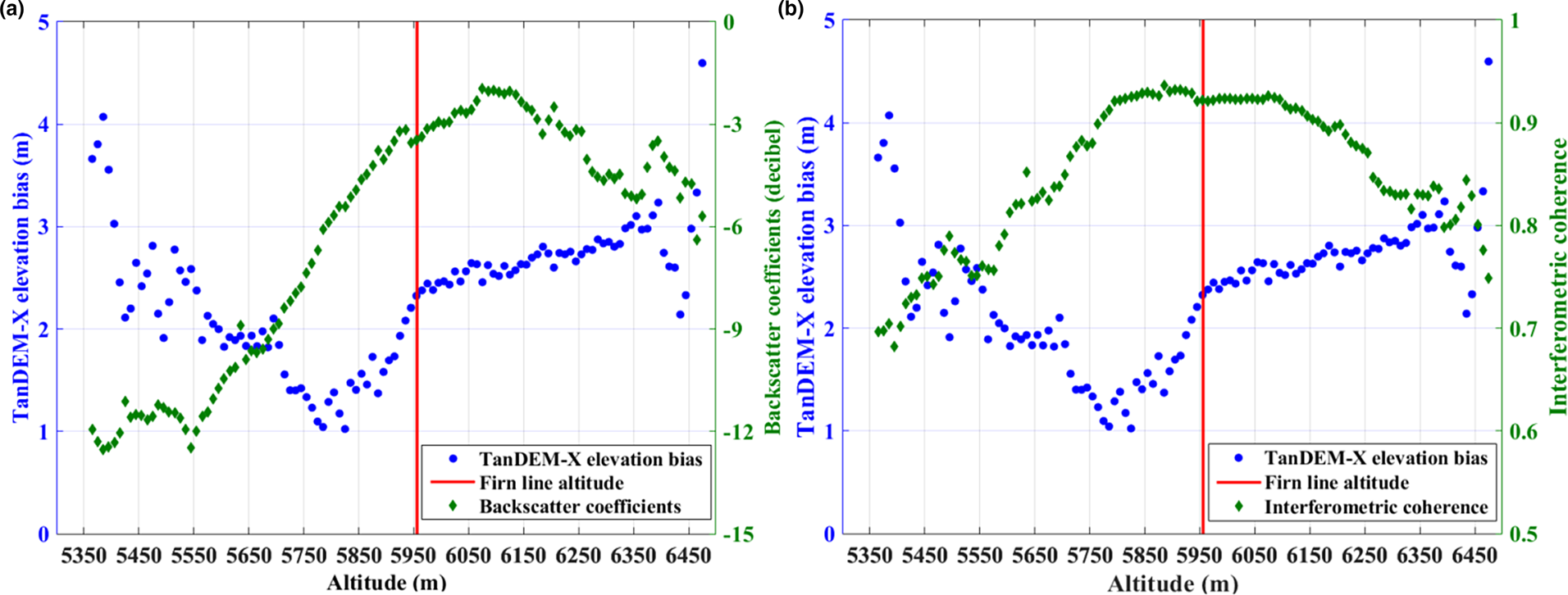
Fig. 9. Average TanDEM-X elevation bias, average backscatter coefficient (unit: decibel) of the TanDEM-X bistatic image (a), and average interferometric coherence of the TanDEM-X bistatic image pair (b) within every 10-m altitude band for glaciers 1–5 in site 1. The TanDEM-X image was acquired on 16 April 2014.
Water content can elevate the dielectric contrast relative to air (Seehaus and others, Reference Seehaus, Marinsek, Helm, Skvarca and Braun2015; Lambrecht and others, Reference Lambrecht, Mayer, Wendt, Floricioiu and Völksen2018), and is in most cases the major factor that hinders the penetration of microwave signals. In the northern hemisphere, the surface melting of mountain glaciers mainly occurs from May to September (the ablation season). The TanDEM-X images covering sites 1 and 2 in this study were acquired in the middle of April and early October. According to the meteorological data collected by the automatic weather stations that are installed in the middle sections of the Zhazhang Glacier (30°28.57′ N, 90°38.71′ E, Nam Co basin, south Tibetan Plateau) and Parlung No. 4 Glacier (29°14.40′ N, 96°55.20′ E, Parlung-Zangbu river basin, southeast Tibetan Plateau), there should be no significant difference between the air temperature and solar radiation in the middle of April and early October (Zhu and others, Reference Zhu2015). The melting of glaciers at these two points in time is usually moderate. However, October is characterised by transition from the warm season to the cold season, whereas April is characterised by the transition from the cold season to the warm season. The accumulation zone therefore has more fresh and dry snow in April than in October. Furthermore, new snowfall can be observed at site 1 in Figure 1d. Hence, for glacier areas above the firn line, the δ in site 1 is higher than that in site 2 (2.612 ± 0.019 m compared to 1.942 ± 0.020 m).
However, some of the δ observed in the ablation zone cannot be ascribed to microwave penetration. As shown in Figures 9a and b, between 5360 and 5960 m a.s.l., the observed δ first decreases and then increases (with the point of inflexion at 5790 m a.s.l.), whereas the backscatter coefficient and interferometric coherence keep increasing. Between 5360 and 5790 m a.s.l., a higher δ generally corresponds to lower backscatter coefficients and interferometric coherence (Figs 9a, b). The δ observed at the glacier terminus is even higher than it is at the firn line. As mentioned previously, a high penetration depth can lead to low backscatter coefficients and interferometric coherence (Rott and others, Reference Rott, Sturm and Miller1993; Jezek and others, Reference Jezek, Gogineni and Shanableh1994; Hoen and Zebker, Reference Hoen and Zebker2000). However, the prerequisite for this to occur is simple stratigraphy and low water content. The mass heterogeneity and high surface water content at the glacier terminus can greatly hinder microwave penetration. In fact, a significant cause of low SAR backscatter coefficients and interferometric coherence over an exposed glacier body is the presence of surface liquid water, which can absorb signals and aggravate surface decorrelation through specular reflection (Lambrecht and others, Reference Lambrecht, Mayer, Wendt, Floricioiu and Völksen2018). Lower interferometric coherence then leads to lower accuracy of TanDEM-X elevation. The dark view in the tongue areas of glaciers 1–5 in the SPOT-6 false-colour image suggests the presence of surface liquid water (Fig. 1d). To support this hypothesis, we computed the normalised difference water index (NDWI) of site 1 from the multispectral bands of the SPOT-6 image (10 April 2014), and found that the NDWI at the tongue areas of glaciers 1–5 was higher than it was at other areas (Fig. 10). Furthermore, the SAR backscatter coefficients and interferometric coherence generally decrease from the firn line to the glacier terminus (Figs 9a, 9b). As mentioned previously, the amount of surface liquid water generally increases from the firn line to the terminus. Hence, it is highly likely that the prominent δ over the glacier tongues can be ascribed to the InSAR measurement error caused by the presence of surface liquid water.

Fig. 10. NDWI computed from the multispectral bands of the SPOT-6 image (10 April 2014) of site 1. Numbers 1–5 mark the glaciers mentioned in the text.
The baseline decorrelation and shadow can also significantly affect the InSAR measurement in mountainous regions (Zebker and Villasenor, Reference Zebker and Villasenor1992). The SAR systems achieve the image resolution cell by sending a chirp pulse and then sampling the echo. The total scattered field of each slant-range resolution cell is a coherent summation of the radar backscatter from multiple scatterers within the ground-range resolution cell (Lee and Liu, Reference Lee and Liu2001). As the ground-range resolution cell enlarges, the width of the main lobe of the impulse response function increases and then the correlation of the two SAR signals decreases. Given a constant SAR baseline, the ground-range resolution increases as the local terrain slope approaches the nominal radar incident angle (Lee and Liu, Reference Lee and Liu2001). When the local terrain slope equals the nominal radar incident angle, the pixel size becomes infinite and the two SAR signals become totally decorrelated. The baseline correlation (γ baseline) can be computed as follows (Lee and Liu, Reference Lee and Liu2001):
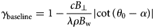
where c, B ⊥, λ, ρ, B w, θ 0 and α are the speed of light, perpendicular baseline, radar wavelength, radar slant-range, range signal bandwidth, nominal incident angle and terrain slope, respectively. The terrain slope facing the radar is positive, while the slope facing away from the radar is negative. The baseline correlation at site 1 is shown in Figure 11. The baseline correlation is relatively low for steep slopes that face the radar illumination (the fore slopes). We set a coherence threshold of 0.5 during the InSAR DEM generation processing and an elevation difference (SPOT-6 DEM - TanDEM-X DEM) threshold of ±20 m to exclude outliers. By combining the elevation difference maps (Fig. 6a) with the baseline correlation map, we can discern that most of the outliers in the elevation difference are caused by the baseline decorrelation. The baseline correlation is usually excellent for slopes that face away from the radar illumination (back slopes); however, the returned radar signals may be very weak. As the local incident angle approaches 90°, the returned signals become increasingly weak (with a lower backscatter coefficient) and the interferometric coherence decreases correspondingly (Lee and Liu, Reference Lee and Liu2001). This explains why the baseline correlation is excellent over some ice-free back slopes, while the δ is prominent there (such as region A in Fig. 6a). Under extreme circumstances, such as the local incident angle being ≥90°, the back slopes become shadowed areas and no information can be gained.

Fig. 11. Baseline correlation of the TanDEM-X interferometric phase in site 1 (16 April 2014). Values of 0 and 1 denote the lowest and highest baseline correlations, respectively.
6.2. Potential impact on geodetic mass-balance measurements
Comparing the TanDEM-X DEMs with the SPOT-6 DEMs obtained within the same week allows a direct estimation of δ. Our results indicate that a significant δ can be expected over exposed glacier surfaces, even during October and April. The impact of δ on annual geodetic glacier mass change rates is related to the length of the observation period. Given an observation period of 10 years and a glacier mass density of 850 ± 60 kg m−3 (Huss, Reference Huss2013), the geodetic mass loss rate in site 1 could be potentially underestimated by 0.179 ± 0.013 m w.e. a−1 if the April TanDEM-X data and optical/laser/GNSS data were used as the historic and new surface elevation sources, respectively. In site 2, the corresponding value would be 0.129 ± 0.010 m w.e. a−1 if the October TanDEM-X data and optical/laser/GNSS data were used as the historic and new surface elevation sources, respectively. The uncertainties of the mass balance are computed based on the uncertainties of the elevation difference and mass density using the basic law of error propagation.
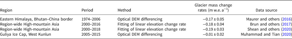
With regards to the distribution pattern and the main impacting factors of the observed δ, we treated the glacier areas below and above the firn line differently when deducing the potential impacts of winter and summer δ on geodetic mass-balance measurements. The X-band penetration over glacier areas above the firn line in winter will be stronger than that in autumn or spring because the water content of the upper layer will be lower and more fresh snow will be preserved. Lambrecht and others (Reference Lambrecht, Mayer, Wendt, Floricioiu and Völksen2018) compared a time series of TanDEM-X DEMs in a low-lying firn basin of the Fedchenko Glacier, Pamir. They found that the winter elevations were consistently lower than the summer elevations by ~6.0 m, and that the autumn (October) elevations were lower than the summer elevations by ~4.5 m. To a large extent, firn densification and the discrepancy between the X-band penetration over wet and dry firn should account for this ‘seasonal change in elevation’, because the mass flows slowly and the melt rates cannot be 5–6 m in this basin (Lambrecht and others, Reference Lambrecht, Mayer, Wendt, Floricioiu and Völksen2018). In our study areas, many glaciers have similar values of δ (3–5 m) in their firn basins during October. Referring to the case of the Fedchenko Glacier, we assumed that, in glacier areas above the firn line, the average δ in autumn or spring is 75% of that in winter. In glacier areas below the firn line, the interferometric coherence of the TanDEM-X bistatic image pair in winter will be higher than that in autumn or spring because the amount of surface liquid water will be lower. Our results show that, in sites 1 and 2, glacier areas below the firn line with an interferometric coherence higher than 0.9 have an average δ of 1.346 ± 0.019 and 0.922 ± 0.017 m, respectively. It is conservative to assume that in sites 1 and 2, the average δ over the glacier areas below the firn line will be 1.346 and 0.922 m, respectively, in the winter because the X-band penetration will be stronger as the amount of surface liquid water decreases (in terms of an exposed glacier). In this case, for a 10-year observation, the mass loss rates in sites 1 and 2 would be potentially underestimated by 0.218 ± 0.016 m and 0.158 ± 0.011 m w.e. a−1, respectively, if the optical/laser/GNSS data and winter TanDEM-X data were used as the new and historic elevation sources (using the glacier mass density mentioned above). Table 5 lists some newly published High-mountain Asia glacier mass change measurements that are not affected by the TanDEM-X bias. The measured glacier mass change rates are even smaller than those potentially caused by TanDEM-X elevation bias in the winter.
Table 5. Recent High-mountain Asia glacier mass-balance measurements
In contrast, the X-band penetration over glacier areas above the firn line in summer will be much weaker than that in autumn or spring because the upper layer is humidified (Huang and others, Reference Huang, Li, Tian, Chen and Zhou2013). Meanwhile, the interferometric coherence will be at a similar level because the surface is not submerged. Hence, we assumed the average δ in glacier areas above the firn line to be zero in summer. Lambrecht and others (Reference Lambrecht, Mayer, Wendt, Floricioiu and Völksen2018) verified that the δ over a firn basin of the Fedchenko Glacier was negligible in September. Over glacier areas below the firn line, δ may be higher in the summer than it is in autumn or spring, because large areas will be saturated and surface decorrelation will be stronger (in terms of an exposed glacier). Our results show that, in sites 1 and 2, over glacier areas below the firn line with an interferometric coherence lower than 0.85, the average δ is 1.714 ± 0.034 and 1.002 ± 0.047 m, respectively. We assumed that in sites 1 and 2, the average δ over glacier areas below the firn line would be 1.714 and 1.002 m in summer, respectively. In this case, for a 10-year observation, the mass loss rates in sites 1 and 2 would be potentially underestimated by 0.063 ± 0.005 m and 0.037 ± 0.003 m w.e. a−1, respectively, if the summer TanDEM-X data and optical/laser/GNSS data were used as the historic and new elevation sources (using the glacier mass density mentioned above). However, our assumptions for summer δ are speculative, and the results need to be further verified by a direct estimate of summer δ. Note that the summer δ is likely to be close to zero over debris-covered glacial areas.
TanDEM-X bistatic imagery is one of the few available data sources with wide coverage and fine resolution that can be used for measuring the glacier mass balance. However, caution must be exercised when conclusions are drawn from the geodetic mass-balance measurements derived from TanDEM-X data, especially when the elevation difference map indicates substantial mass accumulation in high zones. In general, for retrieving the annual geodetic glacier mass balance, it would be better to difference the TanDEM-X elevations from the same season or the optical/laser/GNSS elevations from the summer TanDEM-X elevations (Seehaus and others, Reference Seehaus2016). The use of TanDEM-X images is not recommended for seasonal or monthly geodetic mass-balance measurements, even though the intervals of the TanDEM-X images can be narrowed to 1 month or less, because the difference in the TanDEM-X elevation bias under different conditions can exceed the true changes in the glacier surface elevation over short periods.
7. Conclusions
In this study, we investigated the bias of TanDEM-X elevations (δ) over two mountainous glacial zones on the Tibetan Plateau by differencing TanDEM-X DEMs with SPOT-6 DEMs acquired within the same week. The average April δ over the 175.0 km2 glacier areas in the West Kunlun Mountain Range was 2.106 ± 0.012 m, and the average October δ over the 228.8 km2 glacier area in the Geladandong massif was 1.523 ± 0.011 m. The general distribution patterns of δ were similar in the two glacial sites. As altitude increases from the glacier terminus to the firn line, δ first decreases and then increases. However, as altitude increases from the firn line to the glacier head, δ generally increases. The combination of δ, altitude, backscatter coefficients and interferometric coherence indicates that the δ in the accumulation zone and the upper part of the ablation zone is mainly caused by the microwave penetration, while the δ in the lower part of the ablation zone (glacier tongue) is mainly caused by surface decorrelation that leads to errors of InSAR measurement. Given an observation period of 10 years and a glacier mass density of 850 kg m−3, the glacier mass loss rates in the West Kunlun Mountain Range and Dangula massif would be potentially underestimated by 0.218 ± 0.016 m and 0.158 ± 0.011 m w.e. a−1, respectively, if the winter TanDEM-X data and optical/laser/GNSS data were used as the historic and new elevation sources. Such significant bias is able to distort the conclusions made on the state of the glaciers in High-mountain Asia. However, if the summer TanDEM-X DEMs were used instead, the impact would be much less.
Supplementary material
The supplementary material for this article can be found at https://doi.org/10.1017/jog.2021.15
Acknowledgements
We thank the Journal of Glaciology editorial team, reviewers Romain Hugonnet and Thorsten Seehaus, and one anonymous reviewer for their help in improving the quality of this paper. The presented study was supported by the National Key R & D plans of China (no. 2018YFA0605504); the National Natural Science Foundation of China (no. 41904006); the Strategic Priority Research Program of the Chinese Academy of Sciences (no. XDA20100101); the Hunan Provincial Natural Science Foundation of China (no. 2019JJ50761); the Innovation Foundation of the Shanghai Academy of Spaceflight Technology (no. SAST2018-042); the Postdoctoral Science Foundation of China (no. 2018M630908) and the Innovation Driven Project of Central South University (2020CX036). The TanDEM-X CoSSC images were obtained from the DLR via Project No. jiali_XTI_GLAC6767. The Landsat images were obtained from the USGS (http://earthexplorer.usgs.gov/). The 3 arc-second and 1 arc-second C-band SRTM DEMs were obtained from CGIAR-CSI (http://srtm.csi.cgiar.org/) and the Land Processes Distributed Active Archive Center (https://lpdaac.usgs.gov/products/nasadem_hgtv001/), respectively. The ICESat-2 data were obtained from the Distributed Active Archive Center at the National Snow & Ice Data Center (https://nsidc.org/data/icesat-2). The SPOT-6 data were supplied by the SPOT Image Company (order nos. SO17014342 and SO17014343).


 Open access