


1. INTRODUCTION
High-mountain regions with glaciers act as ‘water towers’ for the lowlands, as they provide meltwater not only to the people living close to the mountains, but also to the lowlands via runoff that recharges the river-fed aquifers. Also, through this runoff, such regions affect global sea level (Bolch and others, Reference Bolch2012). The Karakoram is the fourth largest area of glacier cover on Earth (Dyurgerov and Meier, Reference Dyurgerov and Meier2005), with an estimated glacial area of 18 000 square kilometers (Bolch and others, Reference Bolch2012). This region has a diverse vertical distribution of glaciers, ranging in elevation from 2300 m a.s.l. in the Hunza valley to 6300 m on K2 (Hewitt, Reference Hewitt and Kreutzmann2006).
The Karakoram glaciers are fed by precipitation and avalanche. This precipitation has been increasing at elevations near 2500 and 4800 m, but has maximum values between 5000 and 6000 m (Hewitt, Reference Hewitt2005). Within the region, westerly disturbances in winter bring around two-thirds of the high-altitude snow (Hewitt and others, Reference Hewitt, Wake, Young and David1988) and Indian monsoons in summer bring much of the remaining accumulation (Benn and Owen, Reference Benn and Owen1998; Hewitt, Reference Hewitt2005; Bookhagen and Burbank, Reference Bookhagen and Burbank2010; Palazzi and others, Reference Palazzi, Hardenberg, Terzago and Provenzale2015).
Concerning the terminus positions of these glaciers, mapping and field observations found a 5% retreat in the early 20th century (Hewitt, Reference Hewitt2011). The retreat slowed down in the 1970s, and then stabilized in the 1990s, when those in the high Karakoram starting to advance (Mayewski and Jeschke, Reference Mayewski and Jeschke1979; Hewitt, Reference Hewitt2005). The trend remains variable, with the GRACE satellite gravimetric observations in 2003–2009 showing a net loss in mass of glaciers across the high Asian mountains, but the northwestern part including the Karakoram mountain range showing a gain in mass (Matsuo and Heki, Reference Matsuo and Heki2010). Similarly, digital elevation model (DEM) data acquired from the Shuttle Radar Topographic Mission (SRTM) (Farr and others, Reference Farr2007) and Satellite Pour l'Observation de la Terre (SPOT5) optical stereo imagery show that a slight gain in the mass in the central Karakoram glaciers occurred in the period 1999–2008 epoch (Gardelle and others, Reference Gardelle, Berthier and Arnaud2012).
The Karakoram anomaly may be caused by a higher transport of summer monsoonal moisture that not only increases snowfall at high altitudes, but also increases cloudiness and cooling in summers (Farhan and others, Reference Farhan, Zhang, Ma, Guo and Ma2015; Zafar and others, Reference Zafar2016). Another view is that the reason for the resiliency of Karakoram glaciers could be by these due to a higher contribution of winter snowfall compared with monsoon snowfall (Kapnick and others, Reference Kapnick, Delworth, Ashfaq, Malyshev and Milly2014).
But to better understand the mechanisms of the Karakoram anomaly, we should consider that the Karakoram Range has a relatively high density of surge-type glaciers (e.g. Hewitt, Reference Hewitt1969, Reference Hewitt2007, Reference Hewitt2011; Bhambri and others, Reference Bhambri, Hewitt, Kawishwar and Pratap2017). A surge-type glacier has a recurring active phase, also known as the surging phase, and a quiescent phase. During the active phase, the velocities are higher by a factor of 10–100 over a time period ranging from few months to years. In this phase, the terminal position may advance by up to several kilometers. On the other hand, the quiescent phase, also known as normal flow, can last tens to hundreds of years (Jiskoot, Reference Jiskoot, Singh, Singh and Haritashya2011). Surge dynamics in the Karakoram have thus been extensively studied (Mayer and others, Reference Mayer, Fowler, Lambrecht and Scharrek2011; Quincey and others, Reference Quincey2011; Heid and Kääb, Reference Heid and Kääb2012; Rankl and others, Reference Rankl, Kienholz and Braun2014; Quincey and Luckman, Reference Quincey and Luckman2014; Quincey and others, Reference Quincey, Glasser, Cook and Luckman2015; Paul and others, Reference Paul, Strozzi, Schellenberger and Kääb2017). But it is still not clear whether the Karakoram anomaly has a correlation with the surge dynamics in the Karakoram Range. To answer this question, Copland and others (Reference Copland2011) suggested that the recent positive mass balance in the Karakoram played a role in the doubling in number of new surging episodes during the 14-year period before and after 1990. However, the number of surge-type glaciers in their active phase has decreased since 1999, which is hard to explain only by the changes in mass balance, thus suggesting complexity in the surging mechanisms (Rankl and others, Reference Rankl, Kienholz and Braun2014). In particular, spatial and temporal changes in the thermal regime and the role of meltwater in en- and subglacial hydrology are poorly known for the Karakoram Range. Quincey and others (Reference Quincey, Glasser, Cook and Luckman2015) concluded that neither the thermal, nor the hydrological model of surging can account for the observed surges.
To develop a better model, comprehensive in situ observations would be ideal, but because of the remoteness and logistic issues in the Karakoram, it would be practically impossible to perform extensive in situ observations. Instead, surface velocity maps over the Karakoram Range have been presented (e.g. Rankl and others, Reference Rankl, Kienholz and Braun2014). However, most previous velocity maps are either snapshots of a particular period or they have limited temporal resolution. Hence, the variability in seasonal velocity changes and even the presence of the seasonality itself have been uncertain.
To help clarify the mechanisms associated with glacial dynamics in the Eastern Karakoram Range, we report here on the spatial and temporal variability of glacier velocities with unprecedented resolution in this region. We use the L-band synthetic aperture radar (SAR) images acquired by the Phased Array type L-band Synthetic Aperture Radar (PALSAR) sensors of Advanced Land Observing Satellite (ALOS)-1 and ALOS-2, which can retain higher coherency due to its relatively long wavelength (23.8 cm) and allows us to examine detailed spatiotemporal changes in glacier velocities. The observed velocity variability will also be used as a reference dataset to diagnose if any episodes such as active surging and/or pulse event are ongoing.
2. STUDY AREA
We focus on five glaciers in the Eastern Karakoram Range: the Baltoro, Siachen, Kundos, Gasherbrum and Singkhu Glaciers (Fig. 1). The relatively large size of these glaciers allows us to derive a detailed surface velocity distribution under the available spatial resolution of ALOS-1/2 images.

Fig. 1. Location of the studied glaciers. Spatial–temporal evolution of surface velocities at each glacier is shown separately in Figures 2–6 and in Supplementary materials file (Figs S1–S5). The spatial extent of the overview maps provided in Figures 2–6 are indicated by white rectangles. The ASTER-GDEM was used as a source of elevation in the background. Inset: black and green rectangles show ALOS-1/PALSAR-1 observation paths (523,524) and ALOS-2/PALSAR-2 look IDs (RF2_5 = RLF2_5, RF2_6 = RLF2_6), respectively.
With a length of ~58 km, the Baltoro Glacier is one of the longest glaciers in the Karakoram Range (Copland and others, Reference Copland2009). It is mostly debris-free in its upper reaches, but its debris cover becomes thick and extensive near its terminus (Quincey and others, Reference Quincey2009). Using ASTER imagery and GPS data, the lower most 13 km of the Baltoro Glacier were also examined for surface velocity (Copland and others, Reference Copland2009).
The Siachen Glacier is ~72 km, the longest in the study area. Rankl and others (Reference Rankl, Kienholz and Braun2014) have derived velocity data over Siachen Glacier, but a detailed spatial and temporal evolution of the glacier's velocity has remained elusive. Using multi-satellite images, Agarwal and others (Reference Agarwal2017) examined changes in its area, elevation, mass budget and velocity. The velocity data were, however, limited to one summer pair in 2007 and one winter pair from December 2008 to January 2009, with detailed temporal changes being uncertain.
The Kundos Glacier has two tributaries, with the eastern being ~5 km longer than the western (Figs 1, 2c). Whereas the Kundos Glacier surface velocity was mapped by Rankl and others (Reference Rankl, Kienholz and Braun2014), only one snapshot was given, and its spatiotemporal evolution remains uncertain.

Fig. 2. (a) Spatial and temporal surface velocity changes extracted along the entire length of the centerline of the Baltoro Glacier. Expanded view of individual centerline segments of Baltoro Glacier; (b) upstream portion (49–35 km), (c) central portion (35–16 km), (d) terminal potion (16–0 km) and (e) the Godwin-Austen tributary (red lines indicate the boundary of each segmented centerline portion). The color scale in (a, b, c, d, e, f) indicates the scale for the velocity of the glacier, its various parts and of the overview map. The numbers between the color scales and velocity figures indicate the time in years, and they are labeled at the start of the year, i.e. January. The numbers between the vertical axes of the velocity figures, i.e. between (a) and (b), (c) and (d) and on the right side of figure (e) indicate the corresponding analyzed pair results of master-slave images. The detail of the respective pair dates are given in Table 1 and the corresponding velocity field of each pair are given in Figure S1. The green numbers indicate the master-slave images of beam having the right-looking fine-beam mode (RLF2_6). (f) Surface velocity snapshot of Baltoro Glacier derived from 23 December 2006 and 7 February 2007 data. The black line shows the profile line along which the velocity was calculated and arrows indicate the flow direction of the glacier.
For the Gasherbrum Glacier, a surge has been reported (Mayer and others, Reference Mayer, Fowler, Lambrecht and Scharrek2011; Quincey and others, Reference Quincey2011). We derive the surface velocity evolution during the transition period from the active phase to the quiescent phase, and complement previous findings on the surge dynamics.
The Singkhu Glacier is smaller than the Baltoro, Siachen and Kudos glaciers, and is located at altitudes between 4500 and 5800 m a.s.l. Its seasonal and interannual velocity variability has not been reported before.
3. MATERIAL AND METHODS
The processing method closely follows that of previous studies (Strozzi and others, Reference Strozzi, Luckman, Murray, Wegmuller and Werner2002; Yasuda and Furuya, Reference Yasuda and Furuya2013; Abe and Furuya, Reference Abe and Furuya2015). The pixel-offset (feature/speckle) tracking algorithms are based on maximizing the cross-correlation of intensity image patches. The Gamma software package was used to process the SAR dataset (Wegmüller and Werner, Reference Wegmüller and Werner1997). For the ALOS-1 dataset, we use the fine beam single/dual (FBS/FBD) mode images along the ascending path. Their incidence angle at the center of the image is 38.7°, varying only ~4° from the near range to far range. The FBD data were oversampled in the range direction. The temporal baseline for ALOS-1 varies from 46 to 184 d, while for ALOS-2 it varies from 28 to 196 d (Table 1). For the ALOS-2 data, we use strip mode (SM3) imagery along the ascending path. In ALOS-1 data, Baltoro Glacier was covered by path 524, and the remaining glaciers were studied by using the data along path 523. In ALOS-2 data, the downstream area (from the terminus to ~25 km) of Baltoro Glacier was covered by the right-looking fine-beam mode (RLF2_5, with an incidence angle of 31.4°), whereas the ~25–49 km point of Baltoro and all of the other glaciers were analyzed by using data along the RLF2_6 mode with an incidence angle of 36.3°. The spatial coverage of each satellite is shown in Figure 1.
Table 1. ALOS-1/2 data used in this research. Bold areas show the reference pairs for which various feature tracking parameters are tested (YYYYMMDD)

Result ID column: green numbers indicate the pair IDs covering the upstream part of the Baltoro glacier and Godwin-Austen tributary. For the path 523 (covering Siachen, Kundos, Gasherbrum and Singkhu Glaciers), the count for ALOS-2 data continues for RLF2_6 only. For the path 524 (covering Baltoro Glacier), both the look angles (RLF2_5 and RLF2_6) cover the glacier and the count is indicated with black and green numbers.
To establish the best processing parameters, we selected the image pairs by considering two major factors. First, as the possibility of surface-feature preservation is high in winter, we selected pairs in the winter span (December to March). Second, pairs were selected with the shortest possible temporal baseline (46 d for ALOS-1; 28 and 70 d for ALOS-2 data) (Table 1). While various possibilities of search patch size and sampling interval were tested, the velocity has been derived with a search patch of 128 × 128 pixels (range × azimuth), with a sampling interval of 12 × 36 pixels. We set 3.0 as the threshold of the signal-to-noise ratio. The patches below this level were treated as missing data. The separation between satellite orbit paths and the effect of foreshortening over rugged terrain produces a stereoscopic effect known as an artifact offset (Strozzi and others, Reference Strozzi, Luckman, Murray, Wegmuller and Werner2002; Kobayashi and others, Reference Kobayashi, Takada, Furuya and Murakami2009), which was corrected during the pixel-offset tracking with the use of the elevation-dependent correction. For the DEM, we used the Advanced Space-borne Thermal Emission and Reflection Radiometer (ASTER) global digital elevation model (GDEM) Version 2 (https://gdex.cr.usgs.gov/gdex/).
The velocity was calculated by following the parallel flow assumption (Joughin and others, Reference Joughin, Kwok and Fahnestock1998). The ASTER-GDEM was used to calculate the local topographic gradient unit vector. The detailed surface velocity field of each glacier is given in the Supplementary materials file. To examine the spatial and temporal changes in velocity, we first determined the flowline at each glacier and then averaged the velocity data over the 200 m × 200 m area with its center at each flowline. The velocity errors were estimated by measuring the offsets on stable ground (non-glaciated area) (Pritchard and others, Reference Pritchard, Murray, Luckman, Strozzi and Barr2005; Yasuda and Furuya, Reference Yasuda and Furuya2013; Abe and Furuya, Reference Abe and Furuya2015), and they are 12–17 m a−1 for ALOS-1 data and 20–30 m a−1 for ALOS-2 data. Furthermore, we have divided the Baltoro and Siachen Glaciers into four regions: three regions of the main glacial channel (upstream, central and terminal areas) plus the major tributary (e.g. Godwin-Austen for the Baltoro, Teram Shehr for the Siachen). The lengths of the subregions vary for each glacier, and the start and end of a region were set where we found some notable changes in velocity. This subdivision has not been done for the other three glaciers as there were no such notable changes in velocity along their length.
Pixel-offset tracking by L-band SAR is known to often generate ‘azimuth streaks’ (Gray and Mattar, Reference Gray and Mattar2000; Kobayashi and others, Reference Kobayashi, Takada, Furuya and Murakami2009). In our ALOS-1/2 data, we observed the streaking pattern in many pairs of ALOS-2 but in few of ALOS-1. This is presumably because for ALOS-2, the data acquisition time is mostly in the local daytime, when there is a higher chance of irregularities in the ionosphere due to the higher background total electron content. Moreover, the streaking is more likely to appear in the data collected close to or in the polar regions (Gray and Mattar, Reference Gray and Mattar2000). Furthermore, the amplitude of glacier displacement is essentially proportional to the temporal period between master and slave date, whereas the amplitude of azimuth streaks arises as a snapshot at the time of imaging. The observed glacier velocities are on the order of 100 m a−1 or more, and as such, the ‘azimuth streaks’ did not substantially affect the observed velocity, and are within the errors of the observed velocities. But these streaks are possibly the main reason that ALOS-2 has more error in velocity than ALOS-1.
The ice penetration depth of L-band microwave is ~15 m (Rignot and others, Reference Rignot, Echelmeye and Krabill2001). Here we assume uniform velocity through the ice layer near the surface down to this penetration depth.
4. RESULTS
4.1. Baltoro Glacier
Of the five glaciers, the Baltoro is the only glacier whose detailed velocity evolution has been extensively studied (Quincey and others, Reference Quincey2009). About 35 km from its terminus lies Concordia, where the Godwin Austen Glacier comes down from the north and joins the main channel of Baltoro Glacier. The maximum velocity of ~180 m a−1 occurs just downstream of Concordia and from here the velocity gradually decreases downstream until the terminus (Fig. 3a). To examine the details, we divided the entire glacier into four regions from upstream to downstream (including the Godwin-Austen), and show the velocity evolution of each region separately (Figs 3b, e).

Fig. 3. (a) Spatial and temporal surface velocity changes extracted along the entire length of the centerline of the Siachen Glacier. Expanded view of individual centerline segments of Siachen Glacier; (b) upstream portion (66–40 km), (c) central portion (40–10 km), (d) terminal potion (10–0 km) and (e) the Teram Shehr tributary (red lines indicate the boundary of each segmented centerline portion).The color scale in (a, b, c, d, e, f) indicates the scale for the velocity of the glacier, its various parts and of the overview map. The numbers between the color scales and velocity figures indicate the time in years, and they are labeled at the start of the year, i.e. January. The numbers between the vertical axes of the velocity figures, i.e. between (a) and (b), (c) and (d) and on the right side of figure (e), indicate the corresponding analyzed pair results of master-slave images. The details of the respective pair dates are given in Table 1 and the corresponding velocity field of each pair is given in Figure S2. (f) Surface velocity snapshot of Siachen Glacier derived from 6 December 2006 and 21 January 2007 data. The black line shows the profile line along which the velocity was calculated and arrows indicate the flow direction of the glacier.
These spatial velocity patterns are mostly consistent with those observed by Quincey and others (Reference Quincey2009), although some changes occurred after 2008. The summer speed-up signals are clear every year (Fig. 3a), but are more distinct in the downstream region. For example, the Godwin-Austen Glacier shows no significant summer speed-up signal except for the 2008 summer in its upstream part (Fig. 3e). As Quincey and others (Reference Quincey2009) found for 2005, we see an extra speed-up in 2008, especially in the 10–35 km region (Figs 3a, c, d). However, Quincey and others (Reference Quincey2009) found that the terminal region (0–16 km) did not show significant changes in speed over the period 1992–2008. Except for the lowermost ~5 km, we observe a clear summer speed-up that is extended from the central region (Fig. 3d) in the ALOS-2 data.
Quincey and others (Reference Quincey2009) observed faster speeds in the winter of 2007/2008. Using ALOS1/2 data, we also detected faster winter speeds in the same year (Fig. 3c) as well as in 2014/2015 (Figs 3b, c). However, the speeds are lower in 2008/2009 and 2009/2010. We can observe similar velocity changes in the Godwin-Austen Glacier, indicating faster speeds in the 2007/2008 and 2014/2015 winter seasons (Fig. 3e).
4.2. Siachen Glacier
The velocity along the flowline of the Siachen Glacier decreases gradually from the upstream to the central region and reaches its maximum value between 30 and 40 km upstream from the terminus (Fig. 4a). In this region, we find clear seasonal and interannual variability. Below the 30 km point, the velocity steadily drops until the terminus of the glacier. The small velocity increases at 12 and 20 km probably arise from the tributaries. We again divide the entire glacier into four regions and show the velocity evolution with a different color scale for each part (Figs 4b–e).
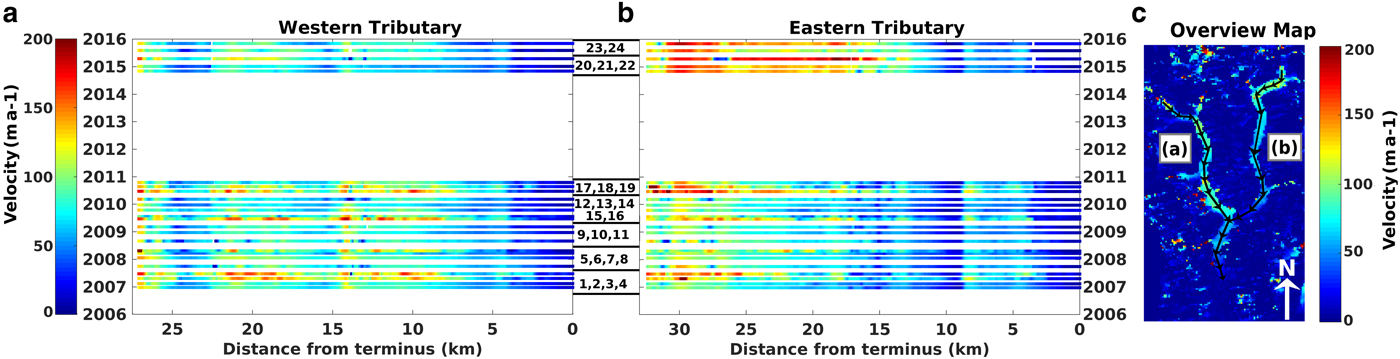
Fig. 4. Spatial and temporal surface velocity changes extracted from the centerline of the (a) western tributary and (b) eastern tributary of Kundos Glacier. (c) Surface velocity snapshot of Kundos Glacier derived from 6 December 2006 and 21 January 2007 data. The black line is a profile line along which the velocity was calculated and arrows indicate the flow direction of the glaciers. After the confluence, i.e. about the 0–9 km area of (a, b), the velocity was calculated along the same line for both parts. The color scale in (a, b) indicates the scale for the velocity of the glacier. The same scale has been used for the overview map as well. The numbers between the color scales and velocity figures indicate the time in years, and they are labeled at the start of the year, i.e. January. The numbers between the vertical axes of the velocity in (a, b) indicate the corresponding analyzed pair results of master-slave images. The details of the respective pair dates are given in Table 1 and the corresponding velocity field of each pair is given in Figure S3.
After 2014, the summer speeds over both the central and upstream regions appear slower than in the previous years (Figs 4a, c). For example, the 2015 summer speed in the central part is below 200 m a−1 and the upstream winter speed is slower than the previous year's by more than 35%. The presence of seasonality in the upstream region is not clear because it often undergoes a decorrelation problem. This problem occurs because the summer snowfall at higher elevations can significantly change the surface features, creating difficulty for the offset-tracking algorithm, and thus making it difficult to measure the velocity (Figs 4a, b). Nevertheless, in the 2009/2010 winter season, the results show a significant speed-up upstream, being nearly twice as high as all other years (Fig. 4b), and also show a speed-up over the central part (Fig. 4c). In contrast, the terminal region has its fastest speed in the 2015 summer, being 30% faster than the 2010 summer when the maximum speed occurs in the central part.
In contrast, Siachen Glacier's largest tributary, the Teram Shehr Glacier, shows very little interannual speed variations over the last 10 years (Fig. 4e). This nearly steady velocity distribution demonstrates that the observed velocity changes in the main trunk are not an artifact of the change of satellite from ALOS-1 to ALOS-2.
4.3. Kundos Glacier
The Kundos Glacier has two tributaries. In the western tributary, the speed gradually decreases from the upstream region until the 23 km location (Fig. 2a), which is at the confluence of upstream tributaries. Then, between 23 and 18 km, the speed increases, and downstream from this, it gradually decreases. Upon passing another confluence ~14 km, it flows faster until about 9 km. After this zone, the speed decreases to the terminus. Thus, there are three segments of velocity pattern that are mostly controlled by incoming flow from tributaries (c.f. Bhambri and others, Reference Bhambri, Hewitt, Kawishwar and Pratap2017; Jiskoot and others, Reference Jiskoot, Fox and van Wychen2017).
The velocity distributions of the eastern tributary are also segmented (Fig. 2b) and controlled by the presence of tributaries. The velocity has a maximum near the 30 km point, which is just below a confluence, then slowly decreases southward. A final increase occurs near 9 km at the main confluence of eastern and western tributaries (Fig. 2b). Below this point, most of the ice flow comes from the western tributary, with the western tributary preventing the inflow from the eastern tributary. Thus, the speed decreases to about zero at 9 km, and then abruptly jumps to the value for the western flowline. After this, both flowlines have the same speed.
Concerning seasonal changes, both tributaries clearly show higher velocities in summer, although the amplitude of peak summer velocity is highly variable. For example, in the western tributary, the summer speeds in 2008 and 2015 are <120 m a−1, whereas those in other years are >150 m a−1 (Fig. 2a). In the eastern tributary (Fig. 2b), the maximum summer speed is 100 m a−1 in 2008, but ~60% faster in the summer of 2010 and over 80% faster in 2015 (even over the 15–25 km portion, where no summer speed-up has been observed previously).
Since 2014, a higher velocity has been detected in the upstream part of the eastern tributary, regardless of the season. The 2014/2015 and 2015/2016 winter speeds are clearly faster by 30% or more than those in previous winter seasons.
4.4. Gasherbrum Glacier
Gasherbrum Glacier underwent a surge that started in fall 2005 and reached its peak velocity of 500 m a−1 during the summer of 2006 (Mayer and others, Reference Mayer, Fowler, Lambrecht and Scharrek2011; Quincey and others, Reference Quincey2011), and is now apparently in its quiescent phase (Fig. 5). Accordingly, the velocity steadily decreases from its upstream region to the terminus. Our data were collected since 2007, and complements the previous studies, showing the transition from the active phase to the quiescent phase in finer detail.
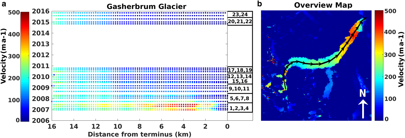
Fig. 5. (a) Spatial and temporal surface velocity changes extracted from the centerline of Gasherbrum glacier. The color scale indicates the scale for the velocity of the glacier. The same scale has been used for the overview map as well. The numbers between the color scale and velocity figure indicate the time in years, and they are labeled at the start of the year, i.e. January. (b) Surface velocity snapshot of Gasherbrum Glacier derived from 6 December 2006 and 21 January 2007 data. The black line is the profile line along which the velocity was calculated and arrows indicate the glacier's flow direction. The numbers at the right side of figure (a) indicate the corresponding analyzed pair of master-slave images. The details of the respective pair dates are provided in Table 1 and the corresponding velocity field of each pair is given in Figure S4.
We observe a slowdown in the winter of 2006/2007, but then a significant acceleration in the summer of 2007, again reaching a velocity of 500 m a−1 (Fig. 5a). The latter peak speed was not reported in Quincey and others (Reference Quincey2011), and indicates that peak velocities occurred both in the summers of 2006 and 2007. In the fall of 2007, the speed decreased to about 250 m a−1, which is consistent with the previous studies (Mayer and others, Reference Mayer, Fowler, Lambrecht and Scharrek2011; Quincey and others Reference Quincey2011). After the active phase, the glacier becomes nearly stagnant in the lower ~10 km portion. Nonetheless, this glacier showed a summer speed-up in 2008 (Fig. 5a). However, the amplitude and spatial extent of the summer speed-up seem to have decreased since 2008.
4.5. Singkhu Glacier
Singkhu Glacier, at an elevation of 4500–5800 m a.s.l., is both relatively high and relatively short compared with the other glaciers. Due to its colder climate, the glacier may be less likely to have short-term velocity changes. However, our measurements show clear summer speed-up signals with interannual modulations, with the fastest speed occurring in the 2010 summer (Fig. 6a). In fact, there are two zones of faster summer velocity, one at 11–14 km and one at 3–10 km. As observed with Kundos Glacier, these two distinct velocity distributions are presumably due to confluences with a major tributary glacier.
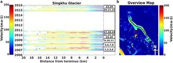
Fig. 6. (a) Spatial and temporal surface velocity changes extracted from the centerline of Singkhu Glacier. The color scale indicates the scale for the velocity of the glacier. The same scale has been used for the overview map as well. The numbers between the color scale and velocity figure indicate the time in years, and they are labeled at the start of the year, i.e. January. (b) Surface velocity snapshot of Singkhu Glacier derived from 6 December 2006 and 21 January 2007 data. The black line is the profile line along which the velocity was calculated and arrows indicate the glacier's flow direction. The numbers at the right side of figure (a) indicate the corresponding analyzed pair of master-slave images. The details of the respective pair dates are provided in Table 1 and the corresponding velocity field of each pair is given in Figure S5.
As we found for the Siachen Glacier, we were not able to derive the upstream velocity in the summer season, which is probably due to the lower image correlation caused by snow accumulation in summer. In 2014–2015, however, we do not observe clear seasonal changes as observed previously, and the maximum summer speed declines, which agrees with that found for the Siachen and western tributary of the Kundos Glacier.
5. DISCUSSION
5.1. Interglacial spatiotemporal velocity variability at seasonal and interannual scales
Our derived velocity data show that both the amplitude and spatial extent of summer speed-up vary from year to glacier. For example, not all the glaciers have their maximum summer velocity in the same year. Moreover, maximum speeds within the same glaciers vary from year to year, which presumably indicates the variability of basal sliding, which is controlled by basal water pressure that depends not only on the input volume of surface meltwater, but also on the capacity of the subglacial hydraulic system at each individual glacier.
Concerning the larger summer speed-ups, Quincey and others (Reference Quincey2009) found an anomalously fast summer speed-up in 2005 at Baltoro Glacier, which was interpreted to indicate additional basal sliding due to the larger volumes of meltwater made available by the deep snowpack in the preceding winter. We found two notable summer speed-ups: one in 2008 at Baltoro Glacier and one in 2010 in the central part of Siachen Glacier. Moreover, we found additional summer speed-up signals, such as on the terminal part of Siachen in 2015 and on the eastern tributary of Kundos in 2015.
All summer speed-ups may be due to a large-volume surface meltwater pulse each spring or summer (c.f. Müller and Iken, Reference Müller and Iken1973; Iken and Bindschadler, Reference Iken and Bindschadler1986). However, this argument is implicitly based on two arguable assumptions: (1) the large surface meltwater pulse is limited to each local glacier at different times, and (2) surface meltwater can efficiently reach the bed and broadly increase basal water pressure during the corresponding same summer.
For the first assumption, we should consider the possibility of heterogeneous climate over the studied area. For such analyses, as surface meteorological data are probably infeasible, one may need to run downscaling analysis of large-scale global numerical weather data (e.g. Bieniek and others, Reference Bieniek2016), considering the complex topography and large elevation differences that can affect the surface weather conditions. However, for the Kundos Glacier, where the close proximity of its tributaries suggests similar surface meteorological conditions, we found that the extra summer speed-up occurred only in the eastern tributary in 2010 and 2015, whereas the western tributary has slowed down since 2015. Instead, the eastern tributary's 2015 speed-up may be a sign of surge initiation, which we will discuss in more detail below. This case suggests that the external meteorological forcing at each glacier does not directly control the summer speed in the same year.
For the second assumption, an efficient passage of meltwater may not be necessary. For example, the summer velocity increases in 2008 at Baltoro, 2010 at Siachen and 2015 at the eastern tributary of Kundos Glaciers were all preceded by relatively fast speeds in the previous winter in their upper regions (Figs 2b, 3b, c, 4b, c). These observations indicate that the extra basal sliding does not necessarily start in the summer, but instead already during the preceding winter in the upstream regions. Although the cause of this upstream speed-up is unclear, once the speed-up occurs, it could help surface meltwater in the following summer to more broadly increase the basal water pressure over the entire glacier. For example, the winter increase in basal sliding would generate more space on the leeward side of bedrock bumps (Kamb, Reference Kamb1987; Schoof, Reference Schoof2010), making the basal water cavities more widely connected when large volumes of meltwater become available in spring to early summer (Iken and Truffer, Reference Iken and Truffer1997).
The question that follows is how the upstream speed-up can be initiated in winter. The winter speed-up in the upstream that precedes a larger summer speed-up is only observed once every several years. The interim time period may be a ‘recharge time’ for the upstream subglacial hydraulic system to generate higher basal water pressure. Unlike the downstream ablation zone, the upstream region generally does not have high volumes of surface meltwater input every summer, and thus it would take longer time to store basal water by either pressure melting of ice like the Svalbard-type thermal regulation (e.g. Murray and others, Reference Murray, Strozzi, Luckman, Jiskoot and Christakos2003) or interstitial englacial water generated by strain heating (Aschwanden and Blatter, Reference Aschwanden and Blatter2005) and their gravity-driven movement as suggested by Irvine-Fynn and others (Reference Irvine-Fynn, Moorman, Williams and Walter2006). Although ice creep will generate locally isolated cavities with high-pressure water, the extra speed-up in winter requires that those cavities become broadly connected, which would also take over 1 year. In this way, the ‘recharge time’ for the upstream winter speed-up would be several years, ultimately leading to the larger summer speeds every several years. The extra summer speed-up preceded by upstream winter speed-up might be better viewed as ‘surge-like’ events reported by Bhambri and others (Reference Bhambri, Hewitt, Kawishwar and Pratap2017).
The recent decrease in summer flow speed at Siachen, the western tributary of Kundos and the Singkhu Glaciers may have occurred because the basal hydraulic system has become more efficient, perhaps due to a long-term larger influx of meltwater reducing the basal water pressure. At the Godwin-Austen Glacier, the absence of a summer speed-up may indicate that either no meltwater could reach the base of glacier (e.g. due to colder ice in the upstream region) or that the morphology of the underlying bed is such that the summer melt does not have an impact on the ice motion.
5.2. Role of hydrological and thermal control mechanisms for flow instability in the Karakoram Range
Surge-type glaciers dominate the Karakoram Range (e.g. Hewitt, Reference Hewitt1969, Reference Hewitt2007, Reference Hewitt2011), but their generation mechanism remains uncertain (e.g. Harrison and Post, Reference Harrison and Post2003; Jiskoot, Reference Jiskoot, Singh, Singh and Haritashya2011; Sevestre and Benn, Reference Sevestre and Benn2015).
To explain differences in surge behavior, Murray and others (Reference Murray, Strozzi, Luckman, Jiskoot and Christakos2003) proposed the Alaskan-type hydrological-regulation and Svalbard-type thermal-regulation mechanisms for the generation of high-pressure basal water that could drive an active surge. In a thermally controlled surge, the initiation and termination phases last for several years before and after the peak phase, respectively, with all phases being independent of the season (Jiskoot, Reference Jiskoot, Singh, Singh and Haritashya2011). On the other hand, hydrologically driven surges are characterized by a rapid acceleration and deceleration, and have a tendency to initiate in winter (Raymond, Reference Raymond1987; Harrison and Post, Reference Harrison and Post2003) and terminate in summer (Björnsson, Reference Björnsson1998). The two models are also entirely different in terms of the origin of basal water. In the hydrological model, the water mainly originates from surface melt, while in the thermal-regulation model, it is generated by pressure melting and frictional heating by the accelerated basal motion without input of surface meltwater. Recent observations, however, suggest that any of these mechanisms cannot be generalized to a study area containing multiple surge-type glaciers (Jiskoot and Juhlin, Reference Jiskoot and Juhlin2009; Quincey and others, Reference Quincey, Glasser, Cook and Luckman2015).
For the Karakoram, Quincey and others (Reference Quincey, Glasser, Cook and Luckman2015) proposed that the surges are part of spectrum from normal slow flow to permanent fast flow, governed by hydrological and basal thermal processes. Moreover, Paul (Reference Paul2015) and Bhambri and others (Reference Bhambri, Hewitt, Kawishwar and Pratap2017) argued that Karakoram glacier surges are only marginally affected by external climate forcing. We find similar behavior in our study area. In particular, Siachen and the eastern tributary of Kundos have shown surge/mini-surge initiation signals independently from each other, indicating that these events are probably not controlled by climate forcing, but rather are the result of internal mechanisms of the glaciers (Raymond, Reference Raymond1987; Jiskoot, Reference Jiskoot, Singh, Singh and Haritashya2011).
Of the five glaciers examined in this study, only Gasherbrum Glacier was surging, and in transition to its quiescent phase. In combination with the previous studies that covered this glacier's earlier phases (Quincey and others, Reference Quincey2011; Mayer and others, Reference Mayer, Fowler, Lambrecht and Scharrek2011), we find that the surface velocities during the active phase turn out to be seasonally modulated with their peak flow in summer. This observation may have an important implication for the Karakoram surge mechanism, particularly because similar seasonal modulation during the active phase has also been found at two glaciers in West Kunlun Shan, northwestern Tibet (Yasuda and Furuya, Reference Yasuda and Furuya2015) and at Hispar Glacier in central Karakoram (Paul and others, Reference Paul, Strozzi, Schellenberger and Kääb2017). In particular, we consider that the seasonal modulation of the peak velocity amplitude is a possible evidence for the role of surface meltwater input to maintain the active phase of polythermal surge-type glaciers; polythermal structure has been assumed by Quincey and others (Reference Quincey, Glasser, Cook and Luckman2015) too. As observed in Karakoram glaciers by Bhambri and others (Reference Bhambri, Hewitt, Kawishwar and Pratap2017), an active surge could generate surface crevasse probably due to the increased longitudinal extensional stress over the glacier through which surface meltwater could easily reach the glacier bed and thereby further enhance the basal water pressure. This process would then help maintain the seasonally modulated active phase. Although it was not a seasonal modulation, Sund and others (Reference Sund, Lauknes and Eiken2014) suggested a similar process for the surge development at the polythermal surge event of Nathorstbreen glacier system, Svalbard.
For Siachen Glacier, the faster flow region initiated in the upstream part of the glacier in early 2010 may have propagated downstream. Although it is not a surge, this is reminiscent of a ‘mini-surge’ or ‘glacier pulse’ observed in Alaskan glaciers (Kamb and others, Reference Kamb1985) and Karakoram glaciers (Bhambri and others, Reference Bhambri, Hewitt, Kawishwar and Pratap2017), or an incomplete surge development as observed for Svalbard glaciers (Sund and others, Reference Sund, Eiken, Hagen and Kääb2009). Because no other examined glaciers revealed similar acceleration in 2010, it is probably not due to any anomalous external climate forcing in 2010, but rather due to local and internal mechanisms at the glacier.
The eastern tributary of Kundos Glacier may have started to surge recently (Fig. 2b). Acceleration occurred in the winter before the maximum speed in the summer of 2015, and this was followed by a velocity decline in the fall of 2015, and another acceleration in the winter of 2015. Even though it may not be a surging episode, the behavior is similar to the surge velocity behavior of Hispar Glacier in the Karakoram, where Paul and others (Reference Paul, Strozzi, Schellenberger and Kääb2017) also noticed a rapid decline in velocity immediately after the maximum speed event in the summer of 2015, with the velocities again increasing significantly in winter 2015–2016 (i.e. after the sudden velocity decline). As Paul and others (Reference Paul, Strozzi, Schellenberger and Kääb2017) suggested for the Hispar Glacier surge, the recent speed-up data at the eastern tributary of Kundos Glacier seems to conform to the Alaskan-type glacial surge model.
Particularly for Alaskan glacier surges, it is known that active phase often initiates in winter (Raymond, Reference Raymond1987). Although there are few reliable reports in Karakoram, Bhambri and others (Reference Bhambri, Hewitt, Kawishwar and Pratap2017) also mentioned a couple of active surges initiated in winter. Furthermore, all the mini-surge events in our study area start in winter as we discussed in the previous section. As winter should have a less efficient basal-drainage system that can more easily generate higher basal water pressure, the initiation in winter may involve subglacial water pooling over a multi-year period due to a combination of basal pressure melting, geothermal heat flux at the bed and/or englacial water storage that can persist over winter (Lingle and Fatland, Reference Lingle and Fatland2003; Abe and Furuya, Reference Abe and Furuya2015).
Although we have separated additional summer speed-up from apparent surging events in this paper, they should lie within the continuous flow-instability spectrum, which much broader than the conventional simple classifications such as ‘surge’, ‘pulse’, ‘mini-surge’ and decadal ‘Svalbard-type’ (Jiskoot, Reference Jiskoot, Singh, Singh and Haritashya2011; Herreid and Truffer, Reference Herreid and Truffer2016). Our essential argument to include both behaviors in this spectrum is that both events are likely controlled by subglacial and possibly englacial hydrology in the upstream region.
5.3. Limitations and recommendations
Our velocity observations demonstrate that the studied Karakoram glaciers are much more dynamically variable in terms of both spatial and temporal evolution than previously reported. Indeed, as our velocity maps are derived from satellite imagery and thus give an average between the acquisition times, the actual velocity changes could be even more dynamic (c.f. Armstrong and others, Reference Armstrong, Anderson and Fahnestock2017). However, our study is confined to the surface velocity data only, and we have not considered independent data such as local weather, surface meltwater volume, basal water pressure and basal topography. Thus, the mechanisms we argued here are speculative. Nonetheless, we believe that the observed diverse range of surface velocity variations will have important implications for future studies, not only at glaciers in Karakoram but also other regions in the world.
To prove or reject our hypotheses, we need not only to extend the time coverage of velocity observations, but also to collect local weather data and analyze the spatiotemporal evolution of weather data. Further testing should also involve direct measurements of basal water pressure in the upstream region over several years. Besides the collection of ground-based meteorological and hydrological observations and their comparative analysis with glacier dynamics at selected sites, modeling studies that can couple glacial hydrology with ice dynamics would also be useful. While there are already some pioneering studies that could quantitatively explain the observations at both mountain glaciers and ice sheets (e.g. Kessler and Anderson, Reference Kessler and Anderson2004; Pimentel and Flowers, Reference Pimentel and Flowers2010; Pimentel and others, Reference Pimentel, Flowers and Schoof2010; Hewitt, Reference Hewitt2013; Hoffman and Price, Reference Hoffman and Price2014; Kyrke-Smith and others, Reference Kyrke-Smith, Katz and Fowler2015; Hoffman and others, Reference Hoffman2016), most studies have focused on the summer speed-up signal attributable to the meltwater input in the same year. Any future model that couples subglacial hydrology with ice dynamics may need to include not only the downstream ablation zone, but also the upstream accumulation zone, and to extend the time coverage for the development of the hydrological system from years to decades.
6. CONCLUSIONS
We applied offset tracking techniques to most of the available L-band SAR data of ALOS-1/2 to determine the surface-velocity trends of five glaciers in the Eastern Karakoram Range over the period 2007–2015. The glaciers show clear seasonal changes in velocity, but with interannually modulated amplitudes and varied spatial extents. Trends for each glacier appeared independent of the others, indicating that their velocities are probably controlled by local and internal mechanisms. The input from tributaries created upstream bands of lower speed, leading to a segmentation of the velocity trends along the length of the glaciers.
We found that Baltoro Glacier had a velocity increase in the summer of 2008 in its central part and an overall speed-up in its upstream part in 2015–2016, whereas Siachen, Singkhu and the eastern tributary of Kundos Glaciers had a speed-up in the summer of 2010. For Siachen Glacier, the longest tributary, Teram Shehr, had a nearly steady velocity distribution throughout the study period. Since 2014, the western tributary of Kundos Glacier slowed down, while in the eastern tributary speed-up, signals were observed over the upstream part, starting in winter and reaching a peak velocity in the summer of 2015. For Siachen Glacier, the upstream and central parts slowed, while the terminal part had an overall acceleration. On the basis of available data, the velocity changes observed at Siachen and eastern tributary of Kundos Glaciers are interpreted as a mini-surge, suggesting the Alaskan-type surge mechanism. The peak velocities of the Gasherbrum surge were seasonally modulated with two maxima in the summers of 2006 and 2007.
Concerning the mechanisms for flow variability, we argue that the intra/interspatial and temporal changes in englacial/subglacial system of each glacier may vary the input of surface meltwater to the base and result in diverse velocity patterns in these glaciers. Our surface-velocity findings show intriguing variations, but their temporal resolution and duration are not sufficient to understand the processes of glacier dynamics fully. To more quantitatively interpret the detailed interannual modulation of seasonal velocity variations, we need to acquire regional high-resolution meteorological and hydrological data as well as run numerical modeling that can fully couple ice dynamics with multi-year englacial and subglacial hydrology.
AUTHOR CONTRIBUTIONS
MU processed, analyzed and produced the results for the ALOS-1/2 data. Both MU and MF have managed the research and drafted this manuscript. Both authors have read and agree with the content of this paper.
SUPPLEMENTARY MATERIAL
The supplementary material for this article can be found at https://doi.org/10.1017/jog.2018.39
ACKNOWLEDGEMENTS
We acknowledge two anonymous reviewers and the Scientific Editor, whose comments were helpful to revise the original manuscript. We are grateful to our colleagues Takatoshi Yasuda and Takahiro Abe for their useful comments. PALSAR-1/2 data were provided by the PALSAR Interferometry Consortium to Study our Evolving Land surface (PIXEL). Ownership of PALSAR-1/2 data belongs to the Japan Aerospace Exploration Agency (JAXA) and the Ministry of Economy, Trade and Industry (METI/Japan).


 Open access