


1. INTRODUCTION
Large-scale modes of climate variability can arise in a variety of ways. Nonlinear dynamical processes intrinsic to the atmosphere can lead to daily to monthly variability that is characteristic of a random stochastic process (Hasselmann, Reference Hasselmann1976). The thermodynamic coupling of the ocean-atmosphere system has the ability to produce slower (interannual and longer) modes of climate variability due to the high thermal inertia of the ocean (Frankignoul and Hasselmann, Reference Frankignoul and Hasselmann1977). Similarly, the response of ocean circulation to wind-stress forcing can lead to decadal modes of climate variability (e.g., Latif and Barnett, Reference Latif and Barnett1994). Regardless of their origin, these modes can exert a large influence on regional and global climate by modifying weather on interannual to multidecadal timescales (e.g., Wigley and Raper, Reference Wigley and Raper1990). Since accumulation and ablation are processes that are impacted by regional variations in precipitation and temperature (e.g., Bitz and Battisti, Reference Bitz and Battisti1999; Roe, Reference Roe2011), the annual or seasonal mass balance of any particular glacier can be strongly affected by climate variability.
Here we examine the influence of climate variability on the seasonal mass-balance records of ten glaciers in Norway, one glacier in Sweden and three glaciers on Svalbard using dynamical adjustment, a statistical technique based on partial least squares regression (PLS regression; Wold and others, Reference Wold, Sjöström and Eriksson2001). Dynamical adjustment reveals the patterns of variability within the mass-balance records that are associated with sea-level pressure (SLP) and sea-surface temperature (SST) anomalies. Once identified, this variability can be regressed out of the records to test a key motivational question: does climate variability affect observed trends in glacier mass-balance records? This set of glaciers span a large geographic area, permitting us to investigate whether a glacier's proximity to common patterns of atmospheric and oceanic variability impacts variability in the records, and whether any long-term trends not associated with fluctuations in SLP and SST variability, such as anthropogenic warming, differ geographically.
1.1. Glacier mass-balance records
The variability that arises from natural fluctuations in the atmosphere and ocean has been shown to force glacier variations in several regions. Despite nearly global retreat of glaciers during the late 20th century (Oerlemans, Reference Oerlemans2005), Pohjola and Rogers (Reference Pohjola and Rogers1997) linked the advance of Scandinavian glaciers during the 1990s to stronger than usual Westerlies in the wintertime and cold summertime flow, which resulted in anomalously high accumulation and low ablation. Huss and others (Reference Huss, Hock, Bauder and Funk2010a) concluded that up to half of the recently observed glacier mass loss in the European Alps is the result of a positive phase of the Atlantic Multidecadal Oscillation (AMO), a pattern of above-normal SST in the North Atlantic which created warm summers, increasing glacier mass loss. More recently, Mackintosh and others (Reference Mackintosh2017) attributed glacier advance in New Zealand from the 1980s to early-2000s to a pattern of atmospheric variability in the extratropical South Pacific that resulted in anomalous southerly winds and low regional SST.
In the era of post-industrial climate change (i.e., since ~1850; Stocker, Reference Stocker2014), glacier mass-balance records reflect both natural and anthropogenic variations, and it is vital to distinguish between the two to extract and understand the response of glaciers to long-term climate changes. An externally-forced trend, such as that due to anthropogenic warming, can be masked by natural variability in the climate system (Medwedeff and Roe, Reference Medwedeff and Roe2017). And although the global aggregate of glacier-length change (Oerlemans, Reference Oerlemans2005) and glacier mass loss (Marzeion and others, Reference Marzeion, Cogley, Richter and Parkes2014) has been cited as evidence of global climate change, attribution with individual records remains challenging: individual glacier mass-balance records are inherently localized climate variables, and few records are longer than several decades (e.g., Braithwaite, Reference Braithwaite2009; Zemp and others, Reference Zemp2015). These two characteristics make them especially susceptible to the effects of circulation-related natural variability, which can bias localized, short-term trends (e.g., Deser and others, Reference Deser, Phillips, Bourdette and Teng2012; Wallace and others, Reference Wallace, Fu, Smoliak, Lin and Johanson2012).
To account for climate variability in glacier mass-balance records and to better understand the remaining trends, more regionally focused studies are needed. The Scandinavian region – the area of interest in this study – is well-suited for examining the effects of climate variability on glacier mass balance. The region is subject to a high degree of climate variability due to the strong coupling between atmospheric and oceanic processes (Marshall and others, Reference Marshall2001), and it is home to numerous glaciers that have multidecadal mass-balance records (WGMS, Reference WGMS2017). Previous studies have assessed the influence of this variability on glacier mass-balance records throughout the region and linked the North Atlantic Oscillation (NAO) to mass-balance variability (e.g., Nesje and others, Reference Nesje, Lie and Dahl2000; Rasmussen and Conway, Reference Rasmussen and Conway2005; Rasmussen, Reference Rasmussen2007; Nesje and others, Reference Nesje, Bakke, Dahl, Lie and Matthews2008; Marzeion and Nesje, Reference Marzeion and Nesje2012; Mutz and others, Reference Mutz, Paeth and Winkler2016). Fluctuations in other climate variables of the region, such as Arctic sea ice, have been linked to both SLP fluctuations associated with the NAO (Deser and others, Reference Deser, Walsh and Timlin2000) and SST variations associated with the AMO (Miles and others, Reference Miles2014; Li and others, Reference Li, Orsolini, Wang, Gao and He2018). Likewise, certain phases of the NAO and AMO have been shown to modulate ice melt on Greenland (Bjørk and others, Reference Bjørk2018; Hahn and others, Reference Hahn, Ummenhofer and Kwon2018). Dynamical adjustment is especially well-suited to assess the impacts of climate variability on glacier mass-balance records in this region because it uses the SLP and SST fields directly, rather than assuming a priori that a particular mode of climate variability dominates over the others.
1.2. Dynamical adjustment
In recent years, dynamical adjustment has emerged as an effective tool for separating the forced and natural components in a number of climate variables. It has been used to analyze the contribution of dynamically induced variability on observed trends in snow pack (Smoliak and others, Reference Smoliak, Wallace, Stoelinga and Mitchell2010; Siler and others, Reference Siler, Proistosescu and Po-Chedley2019), surface temperature (Wallace and others, Reference Wallace, Fu, Smoliak, Lin and Johanson2012; Smoliak and others, Reference Smoliak, Wallace, Lin and Fu2015; Guan and others, Reference Guan, Huang, Guo and Lin2015) and glacier mass balance in western North America (Christian and others, Reference Christian, Siler, Koutnik and Roe2016). This technique has also been applied to evaluate internally generated variability within large climate model ensembles (Deser and others, Reference Deser, Terray and Phillips2016; Lehner and others, Reference Lehner, Deser and Terray2017). In this work, we use PLS-based dynamical adjustment to detect and remove dynamically induced variability in glacier mass-balance records, extending the implementation of Christian and others (Reference Christian, Siler, Koutnik and Roe2016) to a larger set of glaciers in a different geographic region.
Dynamical adjustment identifies the signature of climate variability in glacier mass-balance records under the assumption that circulation anomalies can be identified in a time-varying ‘predictor’ field. The predictors – in this case, SLP and SST fields – are decomposed into patterns that best explain variance in the predictand, which are individual seasonal glacier mass-balance records. Variations in SLP or SST are associated with large-scale circulation anomalies that route precipitation and temperature trajectories, which then have a direct effect on the magnitude of accumulation and ablation. It is important to note that the method does not predefine the spatial patterns of variability that drive glacier mass-balance fluctuations. The spatial patterns are emergent properties determined by the correlation between the glacier mass-balance records (i.e., the predictand) and the SLP and SST fields (i.e., the predictors). Although previous studies have assessed glacier mass-balance variability in terms of circulation anomalies, these studies often rely on climate indices (e.g., Nesje and others, Reference Nesje, Lie and Dahl2000; Huss and others, Reference Huss, Hock, Bauder and Funk2010a) to express dominant modes of pressure and temperature variability (e.g., the NAO or AMO).
The method we apply takes a different approach – we identify climate variability unique to each glacier, which allows us to assess and compare the patterns that drive anomalies in individual mass-balance records. In what follows, we first describe the datasets used in this study and the PLS regression algorithm. We then analyze the raw seasonal glacier mass-balance trends and apply dynamical adjustment to identify climate variability that affects the seasonal mass-balance records. Lastly, we reassess trends across the adjusted mass-balance records and discuss the implications of this work.
2. AREA OF STUDY AND DATASETS
2.1. Predictands: seasonal glacier mass-balance records
Our study includes 14 conventional glacier mass-balance records from Norway, Sweden and Svalbard (see Fig. 1). Conventional mass-balance calculations use the observed glacier area, but since the area of each glacier has evolved over the observational period, the mass-balance records may reflect both climate and glacier dynamics. This has motivated the use of the ‘reference-surface’ mass balance, which fixes the area of the glacier and is a better reflection of climate (Elsberg and others, Reference Elsberg, Harrison, Echelmeyer and Krimmel2001; Leclercq and others, Reference Leclercq, Van de Wal and Oerlemans2010). However, the two methodologies have been shown to agree quite well (Elsberg and others, Reference Elsberg, Harrison, Echelmeyer and Krimmel2001; Huss and others, Reference Huss, Hock, Bauder and Funk2010b). Furthermore, a previous application in which dynamical adjustment was applied to both conventional and reference-surface mass-balance records produced similar results (Christian and others, Reference Christian, Siler, Koutnik and Roe2016). Since the difference between the two approaches is smaller than the uncertainties in the observations, we confine ourselves to the conventional mass-balance records provided by the cognizant measuring agency. We refer to each glacier with indices organized by latitude, with G1 being the most southern glacier and G14 the most northern glacier (see Fig. 1). The Norwegian Water Resources and Energy Directorate (Kjøllmoen and others, Reference Kjøllmoen, Andreassen, Elvehøy, Jackson and Melvold2017) measures the mass balance of glaciers G1–G9 and G11 and contributes these data to the World Glacier Monitoring Service (WGMS, Reference WGMS2017). Several of these records (G1–G9 and G11) include updates based on the reanalysis of Andreassen and others (Reference Andreassen, Elvehøy, Kjøllmoen and Engeset2016). The mass-balance record for Storgläcieren (G10) is maintained by the Bolin Centre for Climate Research (Holmlund and Jansson, Reference Holmlund and Jansson1999). The glaciers on Svalbard (G12–G14) are monitored by the Norwegian Polar Institute (NPI, 2017). Because we are interested in interannual and longer variability, we target mass-balance records long enough to capture decadal fluctuations. Table 1 shows the time period of each glacier mass-balance record considered in this study. The longest continuous records are Storbreen (G3) and Storgläcieren (G10), where the summer mass balance (B s), winter mass balance (B w), and annual mass balance (B a) are available without interruption for nearly 70 years. Although Storgläcieren's mass-balance record starts in 1946, we exclude the first 3-years of the time series as the SLP reanalysis dataset starts in 1948. The shortest record is Langfjordjøkelen (G11), which has a mass-balance record from 1989 to 2016, but is missing data in 1994 and 1995 (Andreassen and others, Reference Andreassen, Nordli, Rasmussen and Melvold2012). Together, the glaciers we select from this region represent one of the longest regional records of glacier response to climate available in the global database (WGMS, Reference WGMS2017).
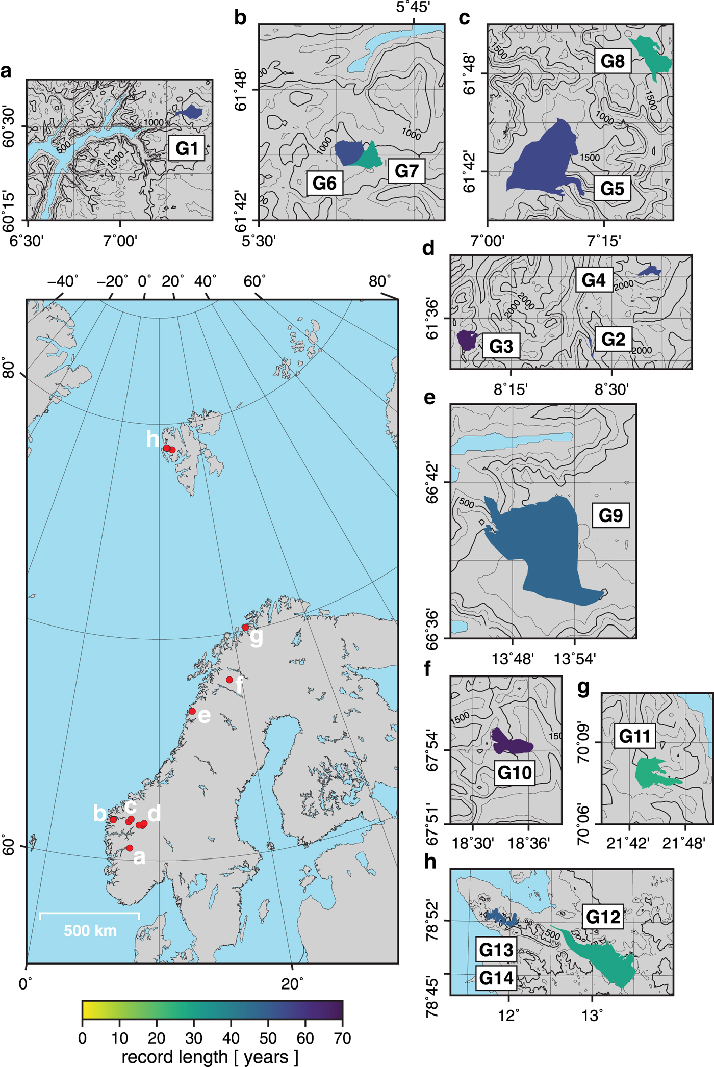
Fig. 1. Location, size and period of the glacier mass-balance records used in this study. Overview map shows the location of the glaciers used in this study. Panels (a–h) are close-ups of individual glaciers. Color shading indicates length of the record (see Table 1). Glacier extents are from the Randolph Glacier Inventory (RGI Consortium, Reference RGI Consortium2017). Contours are elevation intervals of 250 m.
Table 1. A list of the glacier mass-balance records (G1–G14) used in this study, their latitude (°N), elevation (m.a.s.l.), size (km2), period of mass-balance record and mean summer mass balance ( $\overline {B}_{\rm s}$), winter mass balance ( $\overline {B}_{\rm w}$) and annual mass-balance ( $\overline {B}_{\rm a}$) rates during the observational period in meters-water-equivalent per year (m w.e. a−1). For the location of each glacier, see Fig. 1.

In addition to having such long and continuous records, this set of glaciers samples both maritime and continental climate conditions (e.g., Engelhardt and others, Reference Engelhardt, Schuler and Andreassen2015), which allows us to understand the footprints of natural variability in different glacier regimes. Continental glaciers typically have less mass-balance variability, while maritime glaciers, which depend more on precipitation, typically have more mass-balance variability (Medwedeff and Roe, Reference Medwedeff and Roe2017). Table 1 shows the mean mass-balance rates ( $\overline {B}_{\rm s}$, $\overline {B}_{\rm w}$, and $\overline {B}_{\rm a}$) for the 14 glaciers in this study. Maritime glaciers, closer to the ocean, have both high accumulation and high ablation (e.g., Ålfotbreen (G6), $\overline {B}_{\rm w} = 3.62\,{\rm m}\,{\rm w.e.}\,{\rm a}^{-1}$, $\overline {B}_{\rm s} = -3.67\,{\rm m}\,{\rm w.e.}\,{\rm a}^{-1}$). Continental, or inland, glaciers often reflect a drier and colder climate, which is less dictated by variations in precipitation and temperature, resulting in lower magnitude accumulation and ablation values (e.g., Hellstugubreen (G2), $\overline {B}_{\rm w} = 1.10\,{\rm m}\,{\rm w.e.}\,{\rm a}^{-1}$, $\overline {B}_{\rm s} = -1.50\,{\rm m}\,{\rm w.e.}\,{\rm a}^{-1}$). The Arctic glaciers (G12–G14) have low mean winter mass-balance rates of 0.68 m w.e. a−1 and mean summer mass-balance rates of − 1.00 m w.e. a−1, typical values for glaciers in dry polar settings.
Glaciers of different sizes that are located at a variety of elevations (see Table 1) will respond to natural variability and an external forcing in different ways. The diversity in glacier size, mean mass-balance data and geographic locations further highlights the advantage of having a range of glacier mass-balance records to better understand the relationship between atmospheric and oceanic variability and glacier mass-balance fluctuations.
2.2. Predictors: SLP and SST fields
We use two spatiotemporal fields as predictors for glacier mass-balance variability: SLP and SST. In both cases, we use October--March and April--September averages that are similar to the winter and summer mass-balance seasons of the glacier records. The analysis is not particularly sensitive to whether we split the winter and summer averages after April or May. We restrict their spatial domain from 20°N to 90°N and from 65°W to 40°E. We tested various other spatial domains, and our results are not particularly sensitive to the specific domain as long as most of the North Atlantic ocean basin is included so that large-scale circulation variability is captured.
The SLP predictor is a 2.5° × 2.5° grid of monthly means from the NCEP-NCAR reanalysis (Kalnay and others, Reference Kalnay1996). The SST predictor, a 1.0° × 1.0° grid of monthly means, comes from the Met Office Hadley Centre sea ice and sea surface temperature dataset (Rayner and others, Reference Rayner2003). For the SST predictor, we subtract the global mean out of each month to remove the long-term warming signal associated with anthropogenic warming (Flato and others, Reference Flato2014). This retains any trends unique to the North Atlantic region on interannual and multidecadal timescales. We further restrict the SST domain by removing all grid points that experience sea-ice cover (as indicated by the gray hatches in Figs 3, 5).
3. METHODOLOGY
3.1. PLS-based dynamical adjustment
Dynamical adjustment is based on PLS regression, a matrix method that combines features from principal component analysis and multiple regression (Wold and others, Reference Wold, Sjöström and Eriksson2001). The goal of PLS regression is to identify structures in the predictor field, X, that best explain the variance in the predictand, Y. This is done iteratively, where each pass identifies a time series, t, that expresses the amplitude of an associated spatial pattern, W. These structures are analogous to the principal components and associated empirical orthogonal functions of a time-varying field. In PLS regression, however, W is determined by the correlation in time between the predictand and each grid-point of the predictor. In this way, the patterns explain maximal variance in the predictand (though not necessarily in the predictor). To extract the correlated variability, the time series t is projected onto X and Y to determine regression coefficients, P and β. The mode of variability is then regressed out of both the predictor and predictand, leaving adjusted variables:
 $$ {\bf X}_{{\rm adj}} = {\bf X}-{\bf t}{\bf P}^{\rm T }\;{\rm and}\;{\bf Y}_{\rm adj} = {\bf Y}- {\rm \beta} {\bf t} $$
The process is then repeated with Xadj and Yadj to identify and regress remaining patterns of predictor variability that explain variance in the predictand. After multiple iterations, the result is a decomposition of both X and Y into orthogonal modes that have been optimized to explain variance in the predictand. It should be noted that while the regression imposes orthogonality in the time series, these modes are not necessarily physically independent, as it may require more than one fixed spatial pattern to express coherent variations in SLP or SST; alternatively, a single PLS mode may capture variations due to multiple physical processes. These subsequent iterations also tend to explain less variance and eventually fail to yield any physically significant meaning. In this study, we regress only the two leading patterns out of the mass-balance time series. Modes beyond the first two explain little additional variance (< 3%) and do not substantially alter our interpretations and conclusions. For a few records, the second SLP or SST mode explains 1–5% of variance, which we note may not have physically significant meaning. For consistency, we choose to include the first two modes across all glaciers. For comparison, the SLP or SST predictors explain 7–11% of variance in random white noise time series (ranging 30–70 years), which provides a rough threshold for patterns that stand out of the noise. We present the PLS regression algorithm in its entirety in the Appendix, but refer the reader to Smoliak and others (Reference Smoliak, Wallace, Lin and Fu2015) for a comprehensive explanation of PLS-based dynamical adjustment, including discussion on determining the number of modes to retain for a particular analysis.
PLS-based dynamical adjustment provides two useful products for interpretation: first, the patterns that explain variability in both the predictor (SLP or SST) and the predictand (seasonal glacier mass-balance records) can be interpreted as the signature of large-scale circulation variability that is correlated with mass-balance variability. As such, their spatial and temporal components can be compared with both established modes of climate variability and to the predictor patterns for other glaciers (see Section 5). Secondly, by comparing the adjusted mass-balance time series to the raw mass-balance time series, we can assess whether these signatures of climate variability have contributed to observed glacier mass-balance trends.
3.2. Assessing glacier trends and persistence
To evaluate the role of climate variability on glacier mass-balance trends, we assess the magnitude and statistical significance of the seasonal glacier mass-balance trends both before and after dynamical adjustment. We use a two-tailed t-test to evaluate for trend significance (Lettenmaier, Reference Lettenmaier1976). Following Roe (Reference Roe2011), for a given glacier mass-balance record, the t value is given by:
 $$ t = {{\Delta B} \over {\sigma}} \sqrt{ {\nu -2} \over {12}}, $$
where ΔB is the magnitude of the total change in mass balance as estimated by a least-squares linear fit over the observational period, σ is the standard deviation of the detrended residual and ν is the number of degrees of freedom. The signal-to-noise ratio (ΔB/σ) reveals the relationship of a trend with respect to variability, making the significance of a particular trend depends on the signal a glacier exhibits. The trend significance is also statistically dependent on the degree of persistence in the raw glacier mass-balance records, which reduces the degrees of freedom (ν) in the record. The majority of the glacier mass-balance records (G1–G12) we investigate, however, fall below the lag-1 autocorrelation threshold for white noise, defined by Bartlett (Reference Bartlett1946) as  $({1.96})/({\sqrt {n}})$. This result is consistent with the majority of glacier mass-balance records worldwide, which generally lack strong persistence on interannual timescales (Burke and Roe, Reference Burke and Roe2014; Medwedeff and Roe, Reference Medwedeff and Roe2017). Hereinafter, we treat the glacier mass-balance records of G1–G12 as uncorrelated in time and assume that the degrees of freedom in each record equals the number of years in the glacier mass-balance record. To account for the weak persistence in Midtre Lovénbreen (G13) and Austre Brøggerbreen (G14), we estimate ν following Leith (Reference Leith1973), which results in ν = 28 for Midtre Lovénbreen (G13) and ν = 26 for Austre Brøggerbreen (G14) – we evaluate the trend significance accordingly. All critical t values used to determine significance in this study correspond to the 95% confidence level.
4. RESULTS
4.1. Raw mass-balance trends
We begin by assessing the raw (unadjusted) winter and summer mass-balance trends, using the t-test as presented in the previous section (see Table 2). The summer mass-balance of glaciers G1–G7 and G9 show significantly negative trends at the 95% level. Austdalsbreen (G8) and Storgläcieren (G10) also have negative summer mass-balance trends, but both are statistically insignificant. The winter mass-balance trends of G1–G10 are all statistically insignificant, and are also small in magnitude except for Austdalsbreen (G8; − 0.22 m.w.e. a−1 decade−1), but its short record requires a comparatively higher signal-to-noise ratio for trend significance. The glaciers situated further north (G11–G14) show more mixed tendencies. The winter mass balances are all negative, although only Langfjordjøkelen (G11) and Kongsvegen (G12) are statistically significant. Summer mass-balance trends of G11–G14 are all weakly negative and statistically insignificant. The raw mass-balance time series for G1–G14 are presented in the Supplemental Material (see Figs S1 and S2). In summary, the southern set of glaciers (G1–G10) tend to have significantly negative summer mass-balance trends and the northern set of glaciers (G11–G14) tend to have negative winter mass-balance trends, though these are only statistically significant for Langfjordjøkelen (G11) and Kongsvegen (G12). We next apply dynamical adjustment, in order to isolate and remove variability induced by large-scale atmospheric or oceanic circulation, and afterward reassess trends across the adjusted mass-balance records.
Table 2. The seasonal glacier mass-balance trends (m w.e. a−1 decade−1) of the raw and adjusted time series. Values in bold are trends that are statistically significant at 95% based on a two-tailed student's t-test.
4.2. Variability in the winter mass balances
We first consider wintertime (October--March) SLP as a predictor. We find the first two modes explain between 39 and 81% of the variance in winter mass balance (Table 3). Additional modes do not explain appreciable variance (< 3%). Notably, the amount of variability that SLP explains in the winter mass-balance is less (by ~ 30%) in the more northern glaciers (G11–G14) when compared with the more southern glaciers (G1–G10). The amount of variability explained by SLP is also higher (by ~ 20–30%) for the most maritime glaciers (G6–G8) when compared with the more inland glaciers (G2 and G4).
Table 3. Percent (%) of summer and winter mass-balance variability explained in G1–G14 using SST and SLP as predictors. Variance explained is shown for the first mode (M1), second mode (M2) and their sum.

Figures 2 and 3 present the spatial pattern of variability regressed out of the winter mass balances. We focus here on the leading predictor pattern for each glacier but discuss the role of the second mode in Section 5, and provide the patterns of the second mode in the Supplementary Material (see Figs S3 and S4). The first modes of the wintertime SLP predictor patterns are shown in Fig. 2. The leading predictor pattern is nearly identical for glaciers G1–G8, which are clustered within 300 km of each other (Fig. 1); so we show only the mean pattern for G1–G8 in Fig. 2a. For glaciers G1–G8, G9 and G10, the leading predictor pattern has a dipole structure witha negative correlation above 60°N and positive correlation below 60°N. This structure resembles the spatial signature of the NAO (Figures 2a–c; compared with Fig. 9 of Hurrell and Deser, Reference Hurrell and Deser2010). The first mode of the wintertime SLP predictor pattern for Langfjordjøkelen (G11) is noticeably different than the southern set of glaciers (Fig. 2d), with a much less striking dipole. The leading predictor patterns of G12–G14 shows more of a tripole correlation pattern that is reminiscent of the SLP pattern typically associated with the AMO (Figure 2e; compared with Fig. 3 of Knight and others, Reference Knight, Folland and Scaife2006). However, this correspondence is not as close as it is for the southern glaciers and the NAO, which suggests the predictor pattern does not necessarily represent the AMO exclusively; we discuss the relationship between the predictors and established climate modes further in Section 5.
Fig. 2. Predictor patterns for the leading mode of wintertime SLP and the winter mass balance of (a) G1–G8, (b) G9, (c) G10, (d) G11 and (e) G12–G14. The patterns shown for G1–G8 and G12–G14 are both the average of each individual glacier's predictor pattern.
Fig. 3. Predictor patterns for the leading mode of wintertime SST and the winter mass balance of (a) G1–G8, (b) G9, (c) G10, (d) G11 and (e) G12–G14. The patterns shown for G1–G8 and G12–G14 are both the average of each individual glacier's predictor pattern. The hatches mark areas removed from the analysis due to the influence of sea ice. Note that the hatching in (d) covers a smaller area due to Langfjordjøkelen's shorter record; only grid boxes with sea ice since 1989 had to be excluded.
Compared with SLP, wintertime SST explains less mass-balance variability, accounting for 27--54% (Table 3). The first mode of the wintertime SST predictor patterns is presented in Fig. 3. The gray hatches mark areas removed from the analysis due to the influence of sea ice (see Section 2.2). The excluded points differ according to the time period of each mass-balance record; thus the hatches differ across each figure. Like SLP, the SST predictor patterns show a strong south-to-north distinction. For glaciers G1–G8, the SST predictors display a tripole spatial pattern similar to that typically associated with the NAO (Figure 3a; compared with Fig. 2 of Rodwell and others, Reference Rodwell, Rowell and Folland1999). The SST pattern of Engabreen (G9) and Storgläcieren (G10) also share these general NAO characteristics (Figures 3b, c; compared with Fig. 2 of Rodwell and others, Reference Rodwell, Rowell and Folland1999). The leading SST predictor pattern for Langfjordjøkelen (G11; Fig. 3d) is again spatially different than the SST patterns of G1–G10, as a large negative correlation pattern sits off the coast of western Europe that is not seen in the predictor patterns of G1–G10 (Figs 3a–c). The leading SST patterns for the glaciers located on Svalbard (G12–G14; Fig. 3e) depict a region of positive correlation near Svalbard, along with a highly localized negative correlation pattern in the central North Atlantic Ocean basin. This structure is similar, though not identical, to the pattern of G11 (Fig. 3d) and reminiscent of the spatial signature of SST associated with the AMO (Knight and others, Reference Knight, Folland and Scaife2006), which physically manifests as circulation anomalies just south of Greenland near the sub-polar gyre.
4.3. Variability in the summer mass balances
The two leading modes of the summertime (April--September) SLP and SST predictors explain between 24 and 69% of the summer mass-balance variance (Table 3). Circulation in the summertime is less vigorous than in the wintertime, and so, in addition to less variance explained, one may expect that summer mass balance to be more influenced by local radiative effects. Indeed, we find that the predictor patterns do not strongly resemble canonical, large-scale modes of climate variability and are likely associated with regional radiative conditions. The leading SLP and SST predictor patterns for the summer mass balances are shown in Figs 4 and 5, respectively. The second modes are again presented in the Supplemental Material (Figs S5 and S6). For G1–G10, the leading SLP predictor patterns show a center of negative correlation over the Scandinavian region (Figs 4a–c). This is consistent with the persistent anti-cyclonic pressure system that tends to form over Scandinavia in the summer (Luterbacher and others, Reference Luterbacher, Dietrich, Xoplaki, Grosjean and Wanner2004). Such high-pressure systems are associated with clear skies, which result in the availability of more radiation for glacial melt. Similarly, the leading summertime SST predictor patterns (Fig. 5) show local negative correlation in the vicinity of glaciers, but are weak elsewhere. This is consistent with above-normal regional SST that would favor glacier mass loss. Alternatively, the two patterns (Figs 4a–c and 5a–c) could be related: clear weather associated with a persistent high-pressure system would create above-normal SST and enhance incident short-wave radiation on the glaciers in the region.
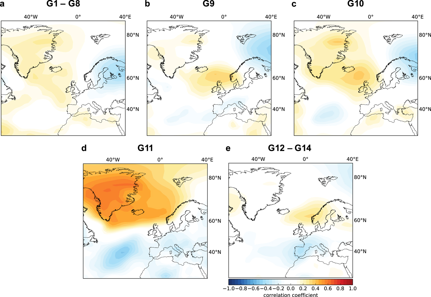
Fig. 4. Predictor patterns for the leading mode of summertime SLP and the summer mass balance of (a) G1–G8, (b) G9, (c) G10, (d) G11 and (e) G12–G14. The patterns shown for G1–G8 and G12–G14 are both the average of each individual glacier's predictor pattern.
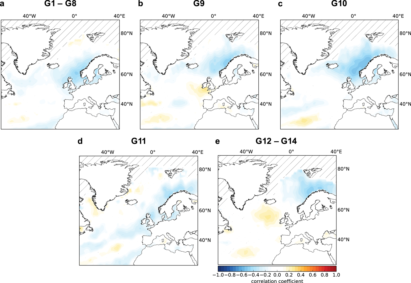
Fig. 5. Predictor patterns for the leading mode of summertime SST and the summer mass-balance of (a) G1–G8, (b) G9, (c) G10, (d) G11 and (e) G12–G14. The patterns shown for G1–G8 and G12–G14 are both the average of each individual glacier's predictor pattern. The hatches mark areas are removed from the analysis due to the influence of sea ice.
4.4. Adjusted mass-balance trends
Our analyses show that between 24 and 81% of seasonal glacier mass-balance variability can be explained by variability in SLP and SST (Table 3). We next evaluate whether these circulation patterns are responsible for some or all of the observed trends in the mass-balance records. Following Smoliak and others (Reference Smoliak, Wallace, Stoelinga and Mitchell2010), we do this by evaluating the trends in the time series after the variability associated with the circulation has been regressed out (shown in Table 2). To illustrate the procedure, Fig. 6 shows the effect of removing, separately, SLP and SST variability on the summer mass-balance of a long-term record, Storbreen (G3) and the winter mass-balance of a short-term record, Langfjordøkelen (G11). For the long-term record, though ~ 43% of the summer mass-balance variability can be explained by SLP or SST variability (Table 3), the significantly negative trend remains largely unchanged (Fig. 6a). Conversely, with a short-term record, the variance explained by SLP or SST (~ 50%) substantially alters the magnitude of the trend (Fig. 6b). The adjusted time series of all of the glaciers are also directly presented in the Supplemental Material (see Figs S1 and S2).
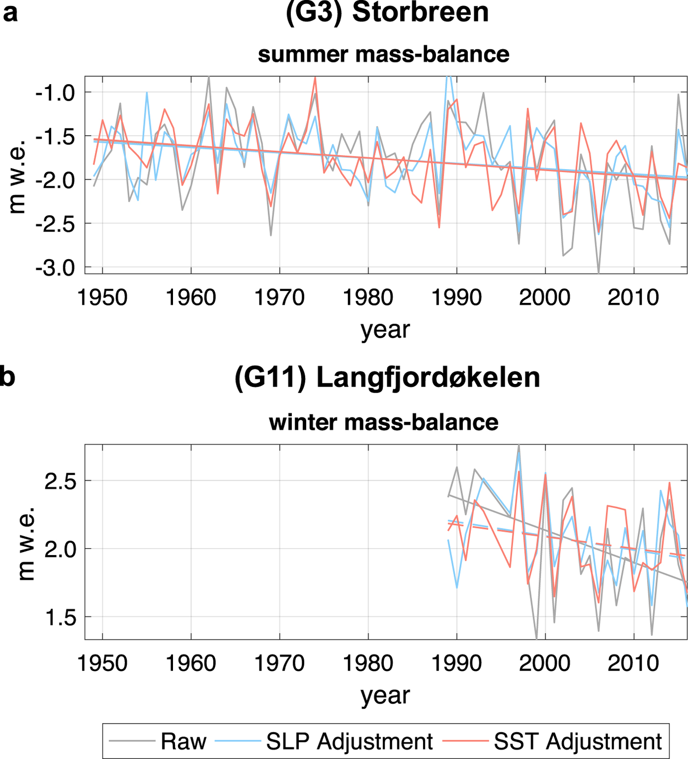
Fig. 6. The raw (gray), adjusted with SLP variability (blue) and adjusted with SST variability (red) summer mass-balance time series for (a) Storbreen (G3) and the winter mass-balance time series for (b) Langfjordjøkelen (G11). The lines represent a least squares linear fit of each time series. The dashed line denotes an insignificant trend and the solid line denotes a significant trend based on the t-test presented in Section 3.
Generally, the summer mass-balance trends do not substantially change after SLP adjustment, although there are a few exceptions. The trends of G1, G3, G5–7 and G9 do remain significantly negative at the 95% level, though most trends become slightly less negative. However, the summer mass-balance trends of Hellstugubreen (G2) and Gråsubreen (G4) remain negative, but drop in magnitude and become statistically insignificant. Notably, the summer mass-balance trends of Austdalsbreen (G8) and Langfjordjøkelen (G11), which both have short mass-balance records (~ 30-years), become significantly negative after SLP adjustment; their negative trends increase in magnitude by ~ 50%. The summer mass-balance trends of G12–G14 remain negative and insignificant, but their trends increase in magnitude. In the winter season, despite accounting for 39–81% of the winter mass-balance variability for G1–G10, SLP anomalies have little effect on the long-term trends; the winter mass-balance trends of G1–G10 remain insignificant, though most trends increase in magnitude. The negative winter mass-balance trend of Langfjordjøkelen (G11), which again has a short mass-balance record, loses statistical significance after SLP adjustment removes ~ 50% of its negative trend (see Fig. 6b). The significantly negative winter mass-balance trend of Kongsvegen (G12) remains significantly negative after adjustment with SLP variance. The insignificant negative winter mass-balance trend of Austre Brøggerbreen (G14) is essentially unchanged, but becomes statistically significant, having lower overall variance. Lastly, the insignificant negative trend of Midtre Lovénbreen (G13) remains insignificant and changes little in magnitude after SLP adjustment.
When using SST as a predictor for glacier mass-balance variability, the adjusted mass-balance trends also remain broadly similar to the raw mass-balance trends with some exceptions. The summer mass-balance trends of G1–G3, G5 and G9 remain significantly negative and change little in magnitude (see Fig. 6a). In contrast, the summer mass-balance trends of G4, G6, and G7 become insignificant and the magnitude of their trends change substantially after SST adjustment. The summer mass-balance trend of both Hansebreen (G7) and Austdalsbreen (G8) change sign. As with SLP, the summer mass-balance trends of G12–G14 remain insignificant and the magnitude of each changes little with SST adjustment. In the winter season, the trends of G1–G9 remain insignificant and the positive winter mass-balance trend of Storgläcieren (G10) becomes significantly positive after SST adjustment. The significantly negative winter mass-balance trend of Kongsvegen (G12) remains and the negative winter mass-balance trend of Austre Brøggerbreen (G14) becomes significantly negative. As with the SLP adjustment, the winter mass-balance trend of Langfjordjøkelen (G11) is reduced by > 50% and loses statistical significance (see Fig. 6b). Lastly, the winter mass-balance trend of Midtre Lovénbreen (G13) remains negative and insignificant after SST adjustment.
5. DISCUSSION
Using dynamical adjustment, we identified and removed variability associated with SLP and SST anomalies from the seasonal mass-balance records of 14 glaciers throughout Norway, Sweden and Svalbard. Our study adds to an already extensive literature (e.g., McCabe and Fountain, Reference McCabe and Fountain1995; Pohjola and Rogers, Reference Pohjola and Rogers1997; Bitz and Battisti, Reference Bitz and Battisti1999; Nesje and others, Reference Nesje, Lie and Dahl2000; Rasmussen and Conway, Reference Rasmussen and Conway2005; Rasmussen, Reference Rasmussen2007; Nesje and others, Reference Nesje, Bakke, Dahl, Lie and Matthews2008; Huss and others, Reference Huss, Hock, Bauder and Funk2010a; Marzeion and Nesje, Reference Marzeion and Nesje2012; Trachsel and Nesje, Reference Trachsel and Nesje2015; Mutz and others, Reference Mutz, Paeth and Winkler2016; Christian and others, Reference Christian, Siler, Koutnik and Roe2016) on the relationship between atmospheric and oceanic circulation and glacier mass balance by identifying patterns of climate variability that best explain mass-balance variability for each glacier. These analyses identify the influence of two prominent modes of variability in the North Atlantic region (i.e., the NAO and AMO) based on the spatial patterns in the leading modes of the predictor fields in the winter adjustments. However, the influences of each are regionally distinct: predictor patterns resembling the NAO drive accumulation variability for the southern glaciers (G1–G10), while patterns spatially resembling the AMO seem to drive accumulation variability for the more northern glaciers (G11–G14). In what follows, we first summarize circulation anomalies that are associated with the canonical NAO and AMO patterns. Then we explore their expression in the winter mass-balance records by comparing the PLS time series with the NAO and AMO indices to quantitatively assess the drivers of accumulation variability. Lastly, we place the results of our study in a broader context by considering the implications of trend changes associated with dynamically induced variability.
5.1. Modes of climate variability
The NAO is a mode of variability that expresses variations in the strength and orientation of the Westerlies, which control moisture and heat transport trajectories in the North Atlantic region (Hurrell, Reference Hurrell1995). The mechanisms creating these variations remain under debate (e.g., Visbeck and others, Reference Visbeck, Hurrell, Polvani and Cullen2001; Hurrell and Deser, Reference Hurrell and Deser2010), but a positive winter NAO phase is associated with low pressure across the high latitudes of the North Atlantic, strengthening the Icelandic low, and high pressure off the coast of western Europe, strengthening the Azores high. This increased south-to-north pressure gradient, drives storm tracks farther north, causing above-normal precipitation over northern Europe and Scandinavia. A negative winter NAO phase is associated with the opposite pressure anomalies over these regions, sending storm tracks farther south and creating below-normal precipitation over northern Europe and Scandinavia (Hurrell and others, Reference Hurrell, Kushnir, Ottersen and Visbeck2003).
Another dominant mode of variability in the region, the AMO, is a coherent pattern of SST variability that is often ascribed a multidecadal signature of 60–80 years, though it is important to note that these anomalies also have substantial power at interannual timescales (see Burke and Roe, Reference Burke and Roe2014). There is ongoing debate about the origins of this variability and whether it arises primarily through the influence of internal atmospheric variability or through changes in ocean circulation (e.g., Clement and others, Reference Clement2015; O'Reilly and others, Reference O'Reilly, Huber, Woollings and Zanna2016). Recent work suggests that the dynamic coupling between atmospheric and oceanic circulations is fundamental to the AMO (Wills and others, Reference Wills, Armour, Battisti and Hartmann2019). Regardless of the underlying mechanisms, the AMO is principally defined in terms of the spatially averaged SST anomalies in the North Atlantic basin (0–60°N, 0–80°W), with a positive (negative) AMO phase identified by above (below) normal SST. AMO variability contributes to anomalously warmer or cooler summers over North America and western Europe (Sutton and Hodson, Reference Sutton and Hodson2005), changes in northern hemispheric mean surface temperature (Knight and others, Reference Knight, Folland and Scaife2006) and Arctic sea-ice variability (Miles and others, Reference Miles2014; Li and others, Reference Li, Orsolini, Wang, Gao and He2018) through the basin-wide redistribution of heat and mass. In the wintertime, a positive AMO phase and above-normal surface temperatures may elevate the rain-snow line, thereby altering the amount of snow accumulation on glaciers.
5.2. Mass-balance variability
The leading SLP and SST predictor patterns for the winter mass balance of the southern glaciers (G1–G10), resemble the spatial signature of the NAO (Figs 2a–c and 3a–c). The relationship between the NAO and accumulation variability has been well-documented (e.g., Pohjola and Rogers, Reference Pohjola and Rogers1997; Nesje and others, Reference Nesje, Lie and Dahl2000; Rasmussen, Reference Rasmussen2007; Nesje and others, Reference Nesje, Bakke, Dahl, Lie and Matthews2008; Mutz and others, Reference Mutz, Paeth and Winkler2016) and it can be interpreted in the light of the storm-track and precipitation relationships described above. The leading SLP and SST predictor patterns of the winter mass-balance of the northern glaciers (G11–G14) exhibit a more AMO-like spatial structure, with a polarity that indicates anti-correlation with the AMO index (Figs 2d, e and 3d, e). However, this pattern is not identical to the AMO and may actually be a blend of different physical mechanisms. For instance, there are also localized positive SST correlations off the coast of Svalbard, suggesting that local SST variations may result in changes to nearby surface temperatures over land. During the winter season, this may allow for stronger storm systems, and thus more accumulation. The influence of the AMO on winter mass-balance variability for the glaciers on Svalbard (G12–G14) is consistent with the spatial extent of the AMO, which influences sea-ice variability near Svalbard (e.g., Day and others, Reference Day, Hargreaves, Annan and Abe-Ouchi2012; Miles and others, Reference Miles2014; Li and others, Reference Li, Orsolini, Wang, Gao and He2018). A mechanistic understanding of how the AMO impacts glacier mass balance in the Arctic may be difficult to partition from circulation variability associated with the NAO. In fact, Wills and others (Reference Wills, Armour, Battisti and Hartmann2019) propose that interannual variability, such as the NAO, is a key driver of the AMO, which suggests that the two modes are intimately related. However, it is worth noting the correlations suggest a negative tendency on winter mass balance occurs when there is a positive AMO phase (above-normal SST). Yet, a positive AMO is associated with an increase in both precipitation and surface temperatures, suggesting that questions remain about the relative importance of accumulation versus winter melt events on high-latitude glaciers and ice sheets.
Since the predictor patterns are not identical to the NAO or AMO, the variability removed from the seasonal mass-balance records likely represent a combination of different modes of climate variability. The PLS time series associated with these spatial patterns can be compared with the temporal indices for the AMO and NAO to further assess the primary drivers of glacier mass-balance variability. In the following, we use October--March averages of monthly NAO and AMO indices from NOAA's Climate Prediction Center (1950-present; Barnston and Livezey, Reference Barnston and Livezey1987) and Earth System Research Laboratory (1948-present; Enfield and others, Reference Enfield, Mestas-Nuñez and Trimble2001), respectively. Figure 7 shows temporal correlations between SLP predictors and the NAO index (Fig. 7a), and SLP predictors and the AMO index (Fig. 7b). Correlations are shown for the two leading PLS time series alone (t1 and t2), and their linear combinations (β 1t1 + β 2t2), the latter of which are the signals ultimately regressed out of the mass-balance records. In general, correlations between the leading PLS time series and the NAO are stronger than with AMO; however, these correlations also show a slight geographic trend of greater influence of the NAO in the south and an anti-correlation with the AMO in the north, especially with the combined modes. For comparison, correlation of the NAO with wintertime precipitation from Norwegian station data is similar (~0.70; Hurrell, Reference Hurrell1995), which adds confidence to the interpretation that the leading PLS mode captures the precipitation signal associated with large-scale atmospheric variability. The remaining variability may be due to local processes (avalanching or wind redistribution) or measurement error. It should be borne in mind that correlations are less robust for the shorter (~ 30-year) records of G7, G8, G11 and G12.
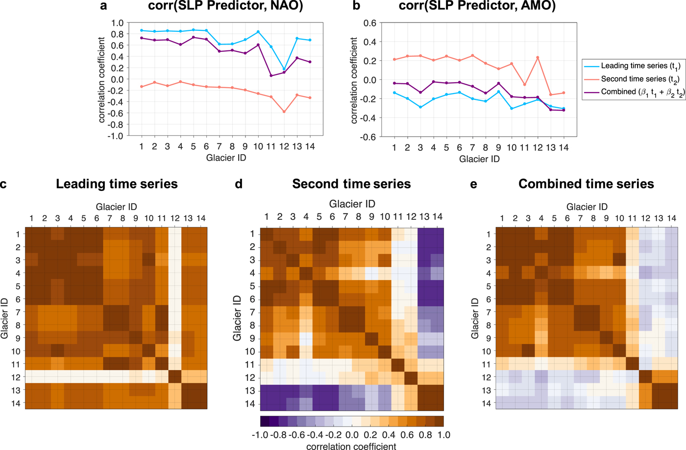
Fig. 7. (a, b) Correlations between climate indices and the SLP predictor time series identified by dynamical adjustment of each winter mass-balance record. Correlations are shown for the two leading time series alone (t1 and t2), and their weighted combinations (β 1t1 and β 2t2). (a) Winter (October--March) NAO index and SLP predictors. (b) Winter AMO index and SLP predictors. (c–e) Inter-glacier correlations of the leading PLS time series (c), the second time series (d) and the combined time series (e). In this case, the second mode helps differentiate the signals of dynamically induced variability between southern and northern glaciers.
The existence of moderate-to-strong correlations across latitudes for both the NAO and AMO suggests that the variability in any mass-balance record is not fully described by a single climate index, but may have multiple origins in the coupled ocean-atmosphere system of the North Atlantic. A combined regression of multiple independent modes, as is done with dynamical adjustment, provides a way to capture this blended variability and also the differing signatures between glaciers. Figures 7c–e displays correlations of the winter SLP time series between pairs of glaciers, again showing the two leading modes alone (Figs 7c–d) and their combination (Fig. 7e). The inter-glacier correlations demonstrate the importance of the second mode for these adjustments: In Fig. 7c, correlations are strong between nearly all glaciers, consistent with some influence of the NAO throughout the region (e.g., Fig. 7a); however, correlations for Fig. 7d have marked differences for southern and northern glaciers. These groups of correlation and anti-correlation also manifest in the combined time series, shown in Fig. 7e. Thus, along with explaining an additional 15–20% of variance in each record (Table 2), these second modes clarify the geographic dependence of mass-balance variability.
These relationships are generally less clear when using SST as a predictor (see Fig. S7 in the Supplemental Material). Because SLP and SST generally have different spatial patterns of variation, the variability identified by dynamical adjustment is not likely to be identically partitioned between the leading modes. The relationships may also be less clear simply because SST is a less robust predictor for mass-balance variability: dynamical adjustments with SST explain less variance than with SLP in nearly all cases (Table 3). The need to remove the global-mean signal as well as any grid-points with sea ice make SST a less-direct and less-expansive indicator of circulation variability for this application. Furthermore, reliably removing the externally forced anthropogenic signal within SST is challenging (e.g., Wills and others, Reference Wills, Schneider, Wallace, Battisti and Hartmann2018) – subtracting the global-mean value at each time step may leave residual regional warming trends. While it can provide a useful check for consistency with SLP adjustments (e.g., noting the influence of AMO/NAO indices in both), we have more confidence in our interpretations of the SLP predictor patterns and time series identified by dynamical adjustment.
5.3. Adjusted trends
After the patterns of variability described above have been regressed out of the original mass-balance records, the adjusted records may more directly manifest long-term trends. Largely, the negative summer mass-balance trends of G1–G9 remain after SST and SLP adjustments, which suggests that the trends are not associated with dynamically induced variability. There are, however, a few notable exceptions. For example, the summer mass-balance trends of Ålfotbreen (G6) and Hansebreen (G7), the two most maritime glaciers in this study, remain negative but become insignificant after adjustment with SST (Table 2). Similarly, the summer mass-balance trends of Hellustubreen (G2) and Gråsubreen (G4) remain negative but become insignificant after SLP adjustment (Table 2). These results suggest that some of the negative summer mass-balance trend may be the result of SST and SLP anomalies not associated with anthropogenic warming. Of course, it is certainly possible that these anomalies may themselves be the forced response, which would suggest that the negative trend will continue. Removing these anomalies make our analysis of any remaining trends a conservative estimate of the anthropogenic signal. Additionally, given the caveats of using SST as a predictor, changes to trend significance due to SST adjustment alone should be interpreted with caution. The negative summer mass-balance trends of Austdalsbreen (G8) and Langfjordjøkelen (G11), which both have short mass-balance records, increase in magnitude and gain statistical significance after SLP adjustment. However, Austdalsbreen is calving into a regulated lake, so caution should be applied when interpreting these trend results since its ablation is influenced to some extent by this regulation (Fleig and others, Reference Fleig2013). Still, this highlights that short-term mass-balance records can be especially susceptible to biases from variability in atmospheric circulation.
For the winter season, the mass-balance trends remain insignificant in the southern group (G1–G9) after both SST and SLP adjustments, though most trends do become slightly more negative. This result indicates that circulation variability while explaining between 27 and 81% of the winter mass-balance variability (Table 3), is not substantially biasing or masking any strong underlying trends. The positive winter mass-balance trend of Storgläcieren (G10), which is insignificant in the raw record, does become significantly positive after adjustment with SST, although not with SLP (Table 2). However, this significance arises mainly through the reduction of variance; the very minor change in magnitude suggests that SST variability is not substantially biasing Storgläcieren's (G10) trend. The geographic tendency of negative winter mass-balance trends for the more Northern glaciers remains after SLP and SST adjustment. The negative winter mass-balance trend of Langfjordjøkelen (G11) is greatly reduced by both SLP and SST adjustment and loses statistical significance, suggesting that climate variability is biasing the trend in its short winter mass-balance record (see Fig. 6b). Lastly, the insignificant winter mass-balance trend of Austre Brøggerbreen (G14) becomes significantly negative once variability from either SLP or SST is removed. However, the tiny change in magnitude suggests that climate variability is not substantially biasing the winter mass-balance trend of Austre Brøggerbreen.
6. SUMMARY AND CONCLUSION
A key challenge in climate science is quantifying the effects of internal variability on climate records (e.g., Hawkins and Sutton, Reference Hawkins and Sutton2009; Deser and others, Reference Deser, Phillips, Bourdette and Teng2012). Glacier retreat is a prominent and tangible manifestation of a warming world and the regional attribution is quite robust (e.g., Roe and others, Reference Roe, Baker and Herla2017). The mass-balance record of any glacier, however, can reflect anthropogenic changes as well as a high degree of variability induced by natural fluctuations of the climate system. Indeed, this means that the variability in any one record may be the result of multiple processes that drive anomalies in accumulation or ablation. This leads to an important prerequisite step before the mass loss of any individual glacier can be attributed to anthropogenic warming: the patterns of large-scale atmospheric and ocean circulation that drive glacier mass-balance variability must be identified and their effect on glacier mass-balance quantified. This work identified that glaciers throughout Norway, Sweden and Svalbard are influenced by the NAO, which is associated with the routing and intensity of winter storms – consistent with several previous studies (e.g., Pohjola and Rogers, Reference Pohjola and Rogers1997; Nesje and others, Reference Nesje, Lie and Dahl2000; Rasmussen, Reference Rasmussen2007; Nesje and others, Reference Nesje, Bakke, Dahl, Lie and Matthews2008; Marzeion and Nesje, Reference Marzeion and Nesje2012; Trachsel and Nesje, Reference Trachsel and Nesje2015). However, dynamical adjustment also revealed that the glaciers residing farther north show progressively more influence of AMO-like anomalies, which suggests that while the NAO is the primary driver of glacier mass-balance variability in the region, both modes of climate variability act to drive anomalies in accumulation. As a large portion of winter mass-balance variability (between 27 and 81%) in this region is driven by patterns reminiscent of these two modes of climate variability, predictions of glacier change may be limited by predictability of the NAO and AMO.
Analysis of trends in the raw and adjusted mass-balance time series is another key result of this study. The glaciers located in southern Norway tend to have significantly negative summer mass-balance trends, whereas the glaciers located farther north tend to have significantly negative winter mass-balance trends. After dynamical adjustment, these seasonal trends largely remain. This suggests that long-term mass-balance trends across the majority of the glaciers in Norway, Sweden and Svalbard has little to do with circulation variability, which stands in contrast to some analyses for glaciers in the Alps, where approximately half of the mass-balance trend is attributable to the AMO (Huss and others, Reference Huss, Hock, Bauder and Funk2010a). The exceptions – where dynamically induced variability more substantially affects mass-balance trends – tend to be those glaciers with shorter mass-balance records or that reside in more maritime climates. This demonstrates the challenges associated with interpreting trends in any single mass-balance record, especially on short timescales. Dynamical adjustment, however, is an effective tool for quantifying these effects as it identifies large-scale circulation patterns that are correlated with glacier mass balances without assuming a relationship to a predefined climate index. Identifying the signature of natural variability will always be a vital step in interpreting trends in glacier mass-balance records. Similar analyses in other regions with multidecadal mass-balance records, such as the Alps, may lead to a more robust understanding of the roles of circulation variability and of anthropogenic forcing on glacier mass balance. Even where long-term glacier mass-balance records are not available, partitioning natural variability from the forced response remains important, and previous applications of dynamical adjustment to temperature and precipitation measurements suggest that it could be applied to investigate the underlying drivers of glacier change in such settings as well.
SUPPLEMENTARY MATERIAL
The supplementary material for this article can be found at https://doi.org/10.1017/jog.2019.35
ACKNOWLEDGMENTS
This work benefited from insightful discussions with Kyle Armour, Cecilia Bitz, and Jack Kohler. We thank Gerard Roe for detailed comments on a draft of this manuscript and Nicholas Siler for offering guidance on the statistical technique. We also thank the Editor, Carleen Tijm-Reijmer and two anonymous reviewers for comments that greatly improved the manuscript. DBB was supported by startup funds from KC at the University of Washington. JEC was supported by the National Science Foundation Graduate Research Fellowship Program (DGE-1256082).
APPENDIX A
Here, we provide additional details on PLS-based dynamical adjustment. As described in the main text, PLS regression is a matrix analysis method that identifies patterns in a predictor, X, optimized to explain variance in a variable of interest, Y, called the predictand. For each adjustment in this study, X is a spatiotemporal SLP or SST field and Y is an individual seasonal mass-balance time series. If n is the number of years in the glacier mass-balance record and m is the number of predictor grid points, then X is a n × m matrix and Y is a n × 1 vector. Both X and Y are standardized to zero mean and unit variance. The spatial pattern W is correlation map using the temporally detrended variables (denoted by X′ and Y′):
 $$ {\bf W} = {{1} \over {n-1}}{\bf X}'^{\rm T} {\bf Y}'. $$
 If W is reshaped back into grid (lat×lon) dimensions, it yields the correlation maps shown in Figs 2–5. Next, X is projected onto  $\big \langle {\bf W}_{\rm c} \big \rangle $, where the brackets denote normalization and Wc is W area-weighted by the cosine of latitude:
 $$ {\bf t} = {\bf X} \big \langle {\bf W}_{\rm c} \big \rangle, $$
where t is a temporal index (with dimensions n × 1) that expresses the variations of the predictor field constrained by its correlation with mass-balance variability. The regression coefficients are, for X, the vector:
 $$ {\bf P} = {\bf X}^{\rm T} \big \langle {\bf t} \big \rangle, $$
and for Y, the scalar:
 $$ \beta = \big \langle {\bf t}^{\rm T} \big \rangle {\bf Y}. $$
Using P and β, t is then regressed out of X and Y, which yields the dynamically adjusted variables:
 $$ {\bf X}_{\rm adj} = {\bf X} - {\bf t}{\bf P}^{\rm T} \; {\rm and}\; {\bf Y}_{\rm adj} = {\bf Y} - \beta{\bf t}. $$
 As noted in Section 3, the regression is then repeated using Xadj and Yadj as inputs, yielding a series of indices t1, t2,  $\ldots $, ti, until further iterations fail to explain appreciable amounts of variance. For each iteration, the variance explained by ti is given by:
 $$ {{{\bf P}_{i}^{\rm T} {\bf P}_{i}} \over {\sum_m\sum_n\vert{\bf X}_{mn}\vert^2}} \; {\rm for}\; {\bf X} \;{\rm and}\; {{\beta_{i}^2} \over {\sum_n\vert{\bf Y}_{n}\vert^2}}\; {\rm for}\; {\bf Y}. $$


 Open access