


1. INTRODUCTION
Globally, glacier meltwater provides water resources for some of the most populated regions on Earth (Barnett and others, Reference Barnett, Adam and Lettenmaier2005). Understanding the driving processes behind meltwater generation is necessary for accurate prediction of water resource availability. While there have been many significant advances in process understanding (e.g. Hock, Reference Hock2005) that are being incorporated into glacier melt models, most of these investigations and modeling efforts have been for glaciers at mid- to high- latitudes (e.g. Pellicciotti and others, Reference Pellicciotti, Ragettli, Carenzo and McPhee2014). By comparison, low latitude glaciers in the tropics are understudied due both to their remoteness and high altitude. In the last 20 years, glaciers located in the tropics have gained interest and have been studied at a few well instrumented sites, such as the Zongo Glacier, Bolivia (Wagnon and others, Reference Wagnon, Ribstein, Francou and Pouyaud1999a, Reference Wagnon, Ribstein, Kaser and Bertonb; Sicart and others, Reference Sicart, Hock, Ribstein, Litt and Ramirez2011), the Antisana Glacier, Ecuador (Francou and others, Reference Francou, Vuille, Favier and Cáceres2004, Favier and others, Reference Favier, Wagnon and Ribstein2004a, Reference Favier, Wagnon, Chazarin, Maisincho and Coudrainb), Kilimanjaro in Tanzania, (Mölg and Hardy, Reference Mölg and Hardy2004; Mölg and others, Reference Mölg, Cullen, Hardy, Kaser and Klok2008), the Lewis Glacier in Kenya (Nicholson and others, Reference Nicholson2010, Reference Nicholson, Prinz, Mölg and Kaser2013) and Artesonraju and Shallap in Peru (Kaser and Osmaston, Reference Kaser and Osmaston2002; Winkler and others, Reference Winkler2009; Gurgiser and others, Reference Gurgiser, Mölg, Nicholson and Kaser2013a, Reference Gurgiser, Marzeion, Nicholson, Ortner and Kaserb). These studies have shown some of the distinct characteristics of the energy balance of tropical glaciers, such as the importance of negative latent heat fluxes on the energy balance during the dry season (Wagnon and others, Reference Wagnon, Ribstein, Kaser and Berton1999b).
To date, one process that has not been explicitly investigated in the scientific literature is the impact of longwave radiation on melting at the lateral margin of tropical glaciers. Based on field observations, it has been noticed that glaciers in mountainous tropical areas seem to retreat not only based on altitude, as a function of air temperature gradients, but also strongly retreat inwards from their lateral margins. This can be seen for the Pastoruri Glacier (Fig. 1), in the Cordillera Blanca (Peru), or the Lewis Glacier (Kenya). Terminal ice cliffs have been investigated by Chinn (Reference Chinn1987) and Lewis and others (Reference Lewis, Fountain and Dana1998) in Antarctica and by Winkler and others (Reference Winkler2010) on Kilimanjaro, but with a focus on the variation of incoming shortwave radiation between the vertical ice cliffs and the flat glacier surface and associated melt.

Fig. 1. Pastoruri Glacier fragmenting in two distinct sections in 2007. Images obtained from the Sociedad Peruano de Drecho Ambiental (a, b, c) and from D. Hoffman (d).
Surrounding terrain, typically from the valley walls and adjacent mountains, influences the longwave radiation budget and the spatial melt patterns at the glacier surface (Marks and Dozier, Reference Marks and Dozier1979; Olyphant, Reference Olyphant1986; Gratton and others, Reference Gratton, Howarth and Marceau1993; Plüss and Ohmura, Reference Plüss and Ohmura1997; Hannah and others, Reference Hannah, Gurnell and McGregor2000). These terrain emissions account for a significant increase of longwave radiation in cold and dry atmospheric conditions at high latitude. For example, in northern Canada, longwave radiation from a south-facing snow-free valley (slope > 35°) was shown to increase longwave radiation on the opposite slope by up to 60% (Sicart and others, Reference Sicart, Pomeroy, Essery and Bewley2006). Moreover, in the Canadian Rockies, terrain irradiance increased longwave radiation 30–50% locally, augmenting local melt by 30% while glacier-wide effects were <6% (Jiskoot and Mueller, Reference Jiskoot and Mueller2012). The process investigated here is similar to terrain longwave radiation, but focused on a smaller scale, where only the terrain up to 15 m away of the glacier impacts the first few meters of the ice (Benn and Evans, Reference Benn and Evans2010).
A comparable process to the margin melt is backwasting from ice cliffs on the debris-covered glacier (Sakai and others, Reference Sakai, Nakawo and Fujita1998, Reference Sakai, Nakawo and Fujita2002; Han and others, Reference Han, Wang, Wei and Liu2010; Reid and Brock, Reference Reid and Brock2014; Steiner and others, Reference Steiner2015; Buri and others, Reference Buri, Pellicciotti, Steiner, Miles and Immerzeel2016). Ice cliff backwasting, which happens when an exposed ice face on the glacier receives increased longwave emission from the surrounding debris, can be an important contributor to overall ablation (Gardelle and others, Reference Gardelle, Berthier, Arnaud and Kääb2013; Pellicciotti and others, Reference Pellicciotti, Stephan, Miles, Immerzeel and Bolch2015; Steiner and others, Reference Steiner2015). We hypothesize that a similar process happens at the glacier margin, where the glacier lateral margin receives enhanced longwave radiation from debris and terrain adjacent to the glacier, and that this process is potentially an important ablation process for tropical glaciers.
The present study investigates the magnitude and spatial variability of the longwave radiation emitted from the rock surface adjacent to a tropical glacier and its impact on the energy balance at the glacier margin and on the total glacier ablation. The longwave flux emitted by the rock adjacent to the glacier is calculated using calibrated ground-based thermal infrared high-definition images of the ablation zone of the Cuchillacocha Glacier, located in the Cordillera Blanca, Peru. The resulting margin longwave flux dataset is incorporated into a distributed energy-balance model of the glacier to assess the relative impact of the longwave flux on the glacier energy balance and melt.
2. METHODS
2.1. Field site and instruments
The Cuchillacocha Glacier (9°24′S, 77°21′W), located at the head of the Quilcayhuanca Valley, ranges in elevation from 4700 to 6096 m a.s.l. (Fig. 2).

Fig. 2. Map of instrumentation deployed at Cuchillacocha Glacier, Peru. Inset box shows site location within Peru. The red box is the area analyzed in the infrared images. The thick black outline is the watershed boundary. Figure adapted from Aubry-Wake and others (Reference Aubry-Wake2015).
The field site and instruments used in this study are the same as described by Aubry-Wake and others (Reference Aubry-Wake2015) with a few additional sensors. An automated weather station (AWS) operated on the glacier ablation zone for the period 23 June to 10 July 2014 at an elevation of 4821 m a.s.l. It recorded incoming and outgoing shortwave radiation, net radiation, air temperature and relative humidity at 0.2 and 1.0 m above the ice level, and surface temperature using an infrared thermocouple sensor with a surface area of 0.5 m2 at 1 min time intervals (Supplementary Fig. S1). Twelve ablation stakes were also deployed within 10 m of the weather station.
Thermal infrared images were taken at 5–10 min intervals for a total of 33 h between 23 and 25 June 2014. The thermal infrared camera was located at an elevation of 4645 m a.s.l. on a moraine facing the glacier, 945 m away from the toe of the glacier and 1145 m from the AWS. The infrared camera, a Jenoptik VarioCam HD with a resolution of 1024 × 768, utilizes an uncooled microbolometer and has a spectral range covering the thermal infrared wavelength of 7.5–14 µm, with a manufacturer's stated accuracy of ±1.5 °C. Pixels for the ablation zone have a 0.64 m2 mean resolution. Air temperature and humidity were recorded at the location of the thermal infrared camera.
At the lowest elevation point along the glacier margin, four temperature sensors were placed at distances of 1, 3, 7 and 10 m from the ice margin. The edge sensors were at the ground surface, under small piles of rocks to maximize the thermal contact between the sensor and the ground. As the sensors were positioned at ground level, their measured temperature is assumed as the ‘true’ surface temperature. The glacier meltwater runs into Cuchillacocha Lake. The discharge from the lake was measured using standard pressure transducer instrumentation. Supplementary Table S1 further describes the instruments deployed at the field site.
The ground-based infrared images were converted to calibrated surface-temperature data following the methodology of Aubry-Wake and others (Reference Aubry-Wake2015). The thermal infrared camera measures radiance, which is a function of the surface temperature, the emissivity of the measured surface and atmospheric transmissivity. Using Plank's law, the radiance is converted to surface temperature. The image processing methodology requires air temperature and relative humidity at the infrared camera location and the glacier AWS, as well as a minimum of three surface temperature control points. These are used to account for interference from the atmosphere and the surroundings, such as reflected radiation from the mountains, turbulent eddies or variable sun exposure. The resulting thermal infrared imagery is a high-resolution, gridded temperature dataset that allows the investigation of small-scale temperature variations at the ground and glacier surfaces.
2.2. View factors
The calculation of the longwave radiation transfer from the rock surface adjacent to the glacier to the ice margin accounts for the geometry of the ice margin using view factors. A view factor is the proportion of the radiation leaving a surface and reaching another surface (Johnson and Watson, Reference Johnson and Watson1984). At the glacier margin, this corresponds to the amount of longwave radiation that reaches the ice face from the adjacent ground surface, which is composed of rock debris of various sizes and sections of exposed bedrock. To define the distance of influence of the ground surface onto the glacier margin, theoretical view factors for 1 m increments leading away from the ice margin are calculated. For each meter away from the margin, a geometric derivation of the view factors, gvf, is calculated (Johnson and Watson, Reference Johnson and Watson1984) (Eqn (1)).
 $$gvf\,(x) = 1 - \; 0.5(x/[x^2 + H^2 ]^{1/2} - 1){\rm \;} $$
where x is the horizontal distance from the top of the glacier slope to the measurement point, here done for 1 m increments from the glacier edge and H is the height of the glacier in meters. The height of the glacier H and the horizontal distance from the top of the slope to the edge of the glacier face A are obtained from the observed geometry of the glacier (Fig. 3). The gvf is obtained as the difference between a fully-unobstructed sky and the calculated sky view factor.

Fig. 3. Schematic of view factor calculation. H is the height of the glacier face, x is the distance from the edge of the glacier to the measurement point, A is the horizontal distance from the top of the slope to the edge of the glacier face and L is the length of the glacier face.
Terrain that is farther from the glacier than a view factor of 0.01 (i.e. <1% of the longwave radiation emitted by the rock is reaching the glacier margin), is considered to have negligible influence on the longwave flux from the rock adjacent to the glacier. Based on a DEM (10 cm resolution) of the ablation zone obtained from UAV data (Wigmore and Mark, Reference Wigmore and Mark2017), the glacier margin wall length (L) in the ablation zone was found to be consistently ~3.0 m long with an inclination θ varying from 30° to almost 90° and most frequently being 75°. Based on this consistently observed margin geometry, this analysis assumes that the glacier margin is uniform in height, with the glacier margin geometry being a wall length (L) of 3 m at an angle of 75°. Our view factor calculation also assumes that surface topography adjacent to the glacier is uniform and flat in the area of interest. Actual ground topography along the edge of the glacier varies slightly from this ideal representation with the presence of boulders, debris mounds or fallen ice blocks. However, we consider that these local variations (boulders, local depression, ice blocks) average each other out when a larger area is taken into consideration (Reid and Brock, Reference Reid and Brock2014).
The glacier view factor decreases exponentially with increasing distance from the glacier. Past a critical distance from the glacier margin, the energy emitted by the rock effectively does not reach the glacier and is instead entirely transferred to the atmosphere. For the glacier edge configuration of a glacier margin face 3 m long at an angle of 75°, the glacier view factor is 0.28 for the first meter away from the glacier margin, then decreases to 0.19 for the second meter and reaches 0.05 at a distance of 5 m from the edge. At a distance of 15 m from the glacier margin, the view factor is slightly below the 0.01 threshold.
2.3. Margin longwave radiation flux calculation
Using the surface temperature dataset obtained from processed ground-based infrared imagery (Aubry-Wake and others, Reference Aubry-Wake2015), the rock surface temperature was extracted for 15 one-meter increments perpendicular to the glacier edge at 350 discrete locations along the ablation zone margin. For each meter step along the transect, the longwave radiation reaching the glacier is calculated using the Stefan–Boltzmann Law. The longwave radiation is then summed for the 15 m transect and divided by the length of the glacier wall L to obtain the longwave radiation reaching the glacier margin from the adjacent rock:
 $$LW_{margin\; discrete} = \sum\limits_{x = 15}^{x = 1} {(gvf_x \varepsilon \sigma T_x ^4 )} /L\; {\rm \; \;} $$
where ε is the emissivity of the surface (0.9), σ is the Stefan Boltzmann constant (5.67 × 10⁻⁸ W m−2 K −4), T is the surface temperature (K) extracted from the thermal infrared images, x is the distance away from the glacier margin and the resulting LW margin discrete is in W m−2. The longwave margin flux LW margin is obtained from the average of all 350 LW margin discrete calculation along the ablation zone. Eqn (2) is also used to compute the longwave margin flux from the surface temperature of the edge sensors for a 14-day period.
2.4. Estimation of the LW margin flux impact on glacier ablation
The impact of the LW margin flux on the ice ablation at the glacier margin is estimated by using a distributed glacier energy-balance model run at an hourly time step with a 30 m × 30 m grid cell resolution. Two versions of the model were used: a base model which is a modified version of the one developed by Rigaudiere and others (Reference Rigaudiere, Ribstein, Francou, Pouyaud and Saravia1995) for the Zongo glacier in Bolivia and a modified version of that model that integrates the LW margin flux in the energy balance at the glacier margin. The difference between the simulation results of the two model versions was used for estimating the ablation triggered by the LW margin flux.
2.4.1. Base model
The base model solves the following energy-balance equation:
 $$M\; = \; SW_{net} + \; LW_{net} + H + LE - C$$
where SW net is the net incoming shortwave radiation, LW net is the net longwave radiation, H and LE are the turbulent sensible and latent heat flux respectively, C is the conductive heat flux and M is the energy available for melt. All terms are in W m−2. A detailed description of equations and parameters is presented in the Supplemental materials.
Input parameters are extrapolated for each cell at an hourly time step from measurements made at the AWSsituated on the glacier. Those include the air temperature measured at two levels (1.0 and 0.2 m above the ice level), the relative humidity, the wind speed and the incoming solar radiation and the atmospheric pressure. Air temperature is extrapolated using a lapse rate of 0.55° 100 m−1 (Gurgiser and others, Reference Gurgiser, Mölg, Nicholson and Kaser2013a). For simplicity, wind speed and relative humidity are assumed to remain constant across the entire glacier. Considering the short distance between the glacier margin and the AWS (200 m), these simplifications were considered reasonable. Direct solar radiation is estimated using the method proposed by Ohta (Reference Ohta1994) and Fierz and others (Reference Fierz, Pluss and Martin1997). The method uses the theoretical maximum solar radiation I c (Garnier and Ohmura, Reference Garnier and Ohmura1968) calculated at each cell as follows:
 $$SW_{in} = \; \displaystyle{{SW_{meas}} \over {I_{cAWS}}} I_{\rm c} $$
where SW in represents the incoming solar radiation for a given cell, SW meas represents the incoming solar radiation measured at the AWS and I cAWS is the theoretical clear-sky solar radiation calculated for the cell that hosts the AWS. The theoretical maximum solar radiation I c calculation includes the terrain effects of the slope and angle of the model grid cell. This also accounts for cloudiness effect, as the calculated incoming solar radiation for each grid cell is scaled to the ratio of measured incoming solar radiation SW meas to the potential clear-sky radiation I cAWS .
SW net is obtained using SW in and a constant albedo throughout the simulation. This is motivated by the short duration of the simulation (2 weeks) and by the fact that no significant precipitation was recorded prior to and during the experiment. Albedo was assigned to individual cells based on their surface type as identified on digital pictures. Albedo of clean dry snow is 0.8, firn at the snow/ice transition is 0.55, clean ice is 0.4, dirty ice at the toe of the glacier is 0.15 and intermediates between clean and dirty ice is 0.3 (Cuffey and Paterson, Reference Cuffey and Paterson2010).
Shade from the surrounding topography may have a great influence on melt generation because incoming solar radiation is the most important source of energy for tropical glacier melt (Nicholson and others, Reference Nicholson, Prinz, Mölg and Kaser2013) and the annual sun path variation is limited in the tropic compared with temperate locations. Where the ice surface is consistently in the shadow of the surrounding mountains, the energy received is significantly reduced. For example, this situation is observed from the positioning of the small tropical glacier, often located in areas of persistent shadows below cliff bands (Kaser and Osmaston, Reference Kaser and Osmaston2002). To account for this phenomenon, a filter based on the topography of the area surrounding the Cuchillacocha Glacier is used in both model versions. The filter modulates the incoming solar radiation received at the surface of the glacier. For each time step, the sun position relative to the studied cell is calculated using sun elevation and azimuth. Where the topography obstructs the incoming solar radiation vector, SW in is turned to 15% of the incoming solar radiation to account for diffuse radiation (Hock and Noetzli, Reference Hock and Noetzli1997) for the cell. Otherwise, SW in is unchanged.
In the base model, the net longwave radiation LW net is calculated as follows:
 $$LW_{net\; \;} = \; LW_{in} - \; LW_{out} $$
where LW in and LW out are the longwave radiation fluxes to and from the glacier surface respectively. Both fluxes are estimated using an empirical equation derived from the Stefan–Boltzmann law (Rigaudiere and others, Reference Rigaudiere, Ribstein, Francou, Pouyaud and Saravia1995). The atmospheric emissivity for LW in was calculated using Brutsaert (Reference Brutsaert1975) while the ice emissivity is 0.985 for LW out .
The turbulent fluxes H and LE are calculated using the Richardson stability coefficient (Kustas and others, Reference Kustas, Rango and Uijlenhoet1994). Because the wind speed is only measured at one level the following assumptions are made:
-
• For H calculation, the wind at 0.2 m above the ice surface is 30% of the one measured at 1.0 m.
-
• For LE calculation, the wind speed at 1 cm is zero. Relative humidity is supposed to remain constant between 0.01 and 1.0 m.
The conductive heat flux C, is calculated for the top 1.5 m of the ice. Underneath this ice layer the ice temperature is assumed to remain at the annual average air temperature. The ice surface temperature is hypothesized to be at the air temperature if the air temperature is negative and at 0°C if the air temperature is at or above 0°C. The 1.5 m top ice layer is divided into five homogeneous sublayers. The conductive heat flux is then computed for each sublayer from the change in cold content with time (Hock, Reference Hock2005).
The energy available for melt, M, is calculated using Eqn (3). It is converted into melt volumes by using the latent heat of melt.
2.4.2. Modified model
In the modified model, the cells situated at the edge of the glacier in the base model are divided into two sub-cells. Only cells in the area analyzed in the infrared images (see Fig. 2) are affected by the modification. The first sub-cell, having an area 10% of the original cell surface, represents the glacier wall (L) described in Section 3.2. For this sub-cell, the modified model is applied. For the second sub-cell, representing 90% of the original cell surface, the model simulate melt using the same energy balance as the base model. In the modified energy-balance equation, the LW net term is replaced by LW net margin that is calculated as follows:
 $$LW_{net\; margin} = \; LW_{in} - \; LW_{out} + \; LW_{margin} $$
where LW margin corresponds to the longwave radiation flux from the ground surface adjacent to the glacier. For practical reasons, all margin sub-cells receive the same value for LW margin at each time step. The value corresponds to the hourly average off all LW calculated at Section 3.3 with Eqn (2).
2.5. Base model performance evaluation
The model performance is evaluated in two ways. First, simulated ice cumulative ablation at the AWS cell is compared with ablation measured using ablation stakes. Second, the cumulative melt simulated for all the glacier cells is compared with the cumulative discharge measured at a gauging station situated at the Cuchillacocha Lake outlet (see Fig. 2).
2.5.1. Ablation measurements
Twelve ablation stakes were deployed in an area of ~10 m2 around the AWS for the 14-day observation period. The average measured ablation of the 12 stakes is used for comparison to the cumulated ablation simulated at the same model cell location. The average ablation measured for the study period was 12 cm with a standard deviation of 3 cm, with individual measurements ranging from 9 to 19 cm. The modeled cumulative ablation simulated with the base model at the AWS cell was 18 cm. Simulation results are within the measurement range with a possible tendency for overestimation. Considering the uncertainty and range of the measurements, the difference between the cell size and the measurement area, and considering that the model results are used in comparison with the modified model simulation only, those results are considered acceptable for the study.
2.5.2. Melt volume measurements
The base model is evaluated by comparing cumulative simulated melt, the output of the melt model, with the measured melt, which is the sum of the measured cumulative lake discharge and calculated lake evaporation. This comparison is made under the assumption that the totality of the melt that occurs at the cells surface drains into the proglacial lake and that the only water losses in the system occur through lake evaporation. Evaporation is calculated using the Penman equation (Abtew and Malesse, Reference Abtew and Malesse2013), using coefficients from Delclaux and others (Reference Delclaux, Coudrain and Condom2007), who calibrated the Penman Equation for Lake Titicaca. The calculated evaporation to measured discharge ratio is 0.14. The comparison between the cumulative simulated melt and the measured melt is presented in Figure 4. The cumulative simulated melt is obtained by first converting the energy available for melt to m w.e. for each glacier cell using a latent heat of fusion of 333.6 J g−1 and an ice density of 920 kg m−1 and then summing all cells to obtain glacier-wide melt.
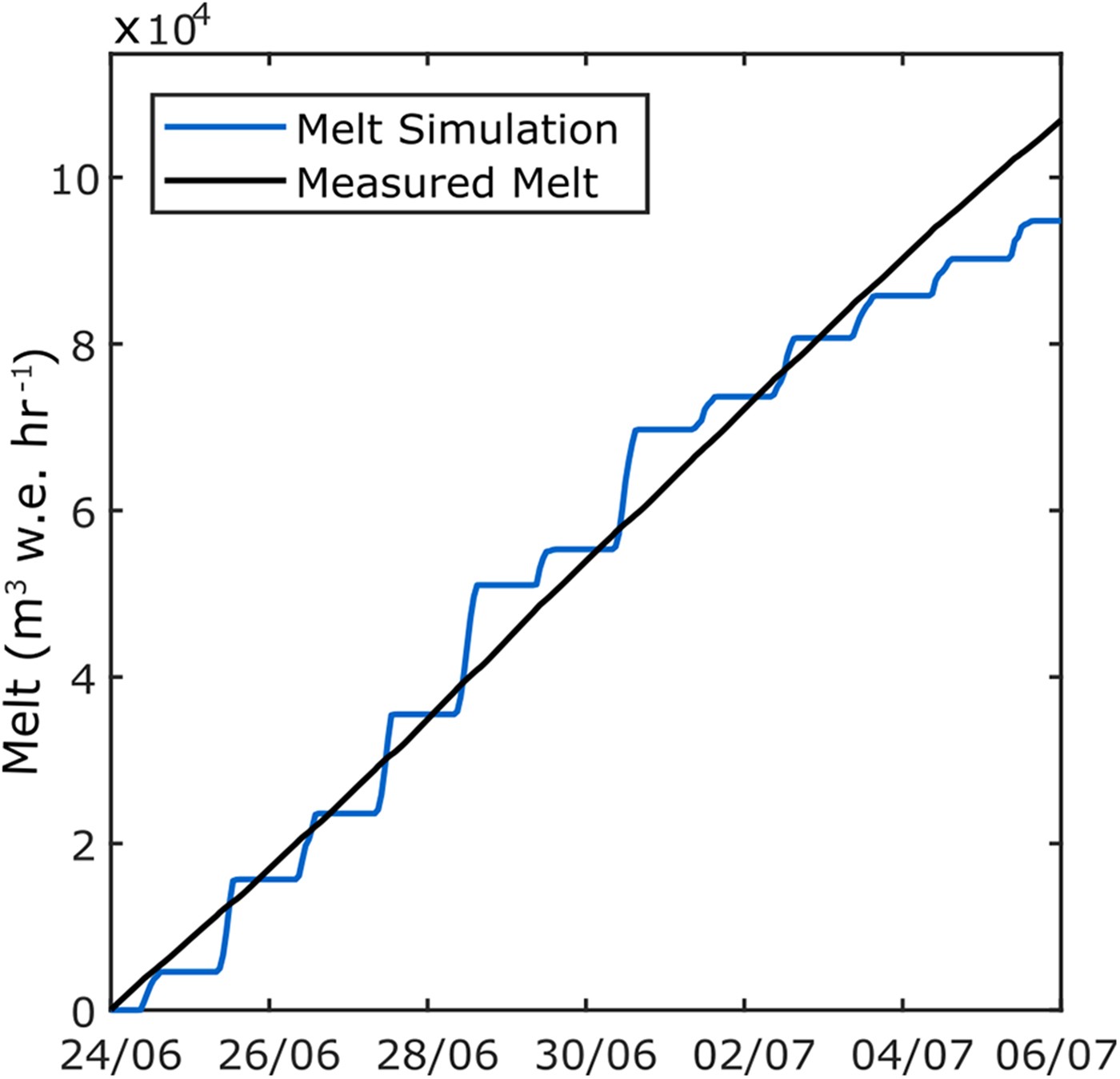
Fig. 4. Comparison of simulated and measured cumulative glacial melt. The blue line is the simulated cumulative melt volume from the base model and the black line is the measured melt (i.e. the sum of the lake discharge and calculated lake evaporation).
The daily simulated melt with the base model from the glacier has an amplitude of 1500 m3 h−1, from zero at night to a peak melt at noon, which results in pronounced daily steps in the cumulated values. The estimated melt, obtained from the measured lake discharge and calculated lake evaporation, does not show these daily steps as both discharge and evaporation have relatively small daily amplitude variations. The lake discharge varies between 302 and 422 m3 h−1 and the evaporation between 26 and 173 m3 h−1. This explains the difference in the pattern of the two lines on Figure 4.
With a correlation coefficient (Pearson's R) of 0. 74, simulated and measured melt volumes, shows an acceptable ability of the base model to reproduce melt volumes during the comparison period. Total cumulative melt volumes at the end of the simulation differ by 13% (Fig. 4), suggesting the model is able to provide a reasonable representation of melt volumes for the purpose of the study.
3. RESULTS
3.1. Spatial variability of margin longwave flux
The margin longwave flux obtained from the infrared images shows a strong daily cyclicity (Fig. 5) over the 33 h of available thermal infrared imagery. The average longwave flux for the ablation zone margin, LW margin , varies between 85 W m−2 at 6:00 AM, the coldest time of the day, and 108 W m−2 ~12:00 PM (noon), the warmest time of the day. It shows a slow cooling trend overnight, decreasing only by 8 W m−2 between 6:00 PM and 8:00 AM. The longwave margin flux increases quickly when the sun appears, reaching 107 W m−2 between 8:00 and 10:00 AM. It then stabilizes until 12:00 PM, the end of the study period.

Fig. 5. Spatial variation of LW margin . Each colored line on (a) is a location where surface temperature was extracted from the thermal infrared images for the 33 h of available imagery, at 5–10 min intervals. The same locations are thin black lines on the infrared images in (b). In (a) and (b), the green dot is the AWS, the yellow dot is the location of the edge temperature sensors and the W and E represent the west and east side of the ablation zone. In (c) each colored line is the LW margin discrete at the corresponding color location in (a). The dashed black line is the longwave radiation calculated at the glacier margin with the edge temperature sensors and the thick black line is LW margin , the average margin longwave flux from all the locations along the ablation zone from the infrared images. Only every third transect from (a) is shown for clarity. The light grey overlay delineates when weather conditions interfered with measurements and the dark grey overlay is when instrument malfunction prevented thermal infrared image acquisition.
The entire ablation margin shows a similar daily fluctuation in LW margin discrete , but the amplitude of daily pattern of the flux depends on the location along the glacier margin. At night, the north side of the glacier (blue on Fig. 5a) is colder, with a longwave flux ranging between 80 and 85 W m−2. For the same period, the west side of the ablation zone (red on Fig. 5a) emits slightly more longwave radiation, between 87 and 92 W m−2. During the day, the opposite pattern happens: the east side of the glacier emits up to 115 W m−2, but the west side reaches only ~92–100 W m−2. On average, the difference between the east and west sides of the glacier is 7 W m−2 overnight, and increases to 28 W m−2 during the day. Both sides of the glacier lie at the same altitude, and thus, the difference in longwave radiation is not related to elevation change. Instead, it appears that the spatial variability of the margin longwave flux is due to local shading effects. Local shading on the ablation zone, obtained from the topography filter in the model (see Section 3.4.1.), shows that in the morning, the east side starts receiving shortwave radiation early in the day (slightly past 8:30 AM) but the west side stays in the shade until past 9:00 AM. In the afternoon, the opposite situation occurs. At 3:30 PM, the west side of the glacier is still in the sunlight and only becomes shaded slightly before 5:00 PM (Fig. 6). Those shading effects have a direct influence on the temperature of the rock adjacent to the glacier affecting the longwave margin flux explaining the variation between the LW margin discrete on the east and west side of the ablation zone.
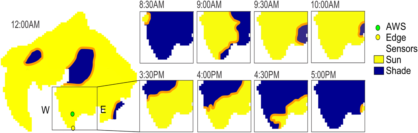
Fig. 6. The shading on the ablation zone for morning and afternoon. Blue is shaded, yellow is receiving incoming solar radiation and orange is the transition zone. E and W represent the east and west sides of the ablation zone.
3.2. LW margin extrapolation in time
For logistical reasons, the infrared images were collected over 33 h only. The measurements are extrapolated to a 14 day period by using the longwave flux calculated from the edge temperature sensors measurements (Fig. 7).

Fig. 7. Extrapolated LW margin (red) from 23 June 2014 to 7 July 2014, based on the linear regression model between the measurements with the infrared images (black) and the edge temperature sensors (dashed black). The square inset is the period where the infrared camera was active. The colored lines within the square are LW margin discrete from all of the location along the glacier margin. The light grey overlay is when weather conditions interfered with measurements and the dark grey overlay is when instrument malfunction prevented thermal infrared image acquisition.
A simple model uses linear regression on the margin longwave fluxes calculated from the temperature edge sensors (black dashed line on Fig. 7) and from the longwave flux calculated from the infrared thermal images (black line on Fig. 7) for the 33 h when both measurements overlap. The longwave flux calculated from the infrared thermal images is the average of the 350 discrete longwave calculations along the glacier margin (Eqn (2)). This linear regression model results in a spatially-averaged longwave margin flux for the 14 days period (red line on Fig. 7). The resulting correlation coefficient (Pearson's R) between the longwave margin flux calculated from the edge temperature sensors and the infrared images is 0.92.
Over the study period, the margin longwave flux fluctuates from a minimum of 85 W m−2 to a maximum of 112 W m−2. The daily pattern consistently shows a sharp increase in the morning, starting as soon as the incoming solar radiation reaches the glacier, ~8:00 AM and either peak ~12:00 AM, or fluctuate ~100 W m−2 until mid-afternoon, due to cloud cover throughout the day. The margin longwave flux then decreases sharply between 4:00 PM and 5:00 PM and then gradually reaches its minimum at 6:00 AM.
3.3. Impacts on surface energy balance
Figure 8 shows the energy available for melt for all the glacier cells as simulated by the modified model for the first day of the experiment. The figure clearly shows an enhanced melt condition at the glacier margin as compared with non-margin areas. The margin regions receive a higher energy available for melt M of ~100 W m−2 between 11:00 AM and 5:00 PM compared with the regions situated away from the margin.
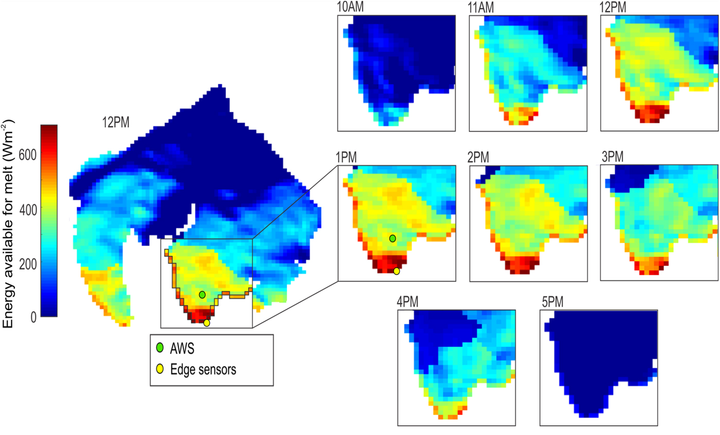
Fig. 8. Energy available for melt M from the modified melt model for 23 June 2014. For visualization purposes, the area impacted by the LW margin , which corresponds to only 10% of the cell on the glacier margin (black outline), was shown as regular sized cells. The green dot is the AWS and the yellow point is the edge sensors location. Only the times when energy available for melt is above zero are shown.
At 10:00 AM, when the glacier starts exhibiting melt areas, the influence of LW margin is not as strong as later on during the day but still perceivable. At 5:00 PM, the model calculates that cells at glacier margin only receive enough energy to generate some melt as all the cells situated away from the margin have zero energy available for melt. The energy available for melt varies along the ablation zone margin, with the highest values observed at the lower portion of the glacier. As the LW margin value was identical for all cells at each time step, the variability seen along the glacier margin results from other factors such as the spatial distribution of the topographic shading, the elevation and/or the albedo.
A comparison of the models’ output for the grid cells at the glacier margin for the 14-days is in Figure 9. Figure 9a shows that the introduction of LW margin into the modified model leads to higher energy for melt during the day but not overnight. Around midday, when energy available for melt is at its maximum for most of the days, the extra energy for melt calculated by the modified model reaches 20% more than that calculated by the base model. The average value for the 10:00 AM to noon window reaches 310 W m−2 for the modified model against 200 W m−2 for the base model. The difference between the model outputs is not only observed in the amplitudes of the energy availability for melt but appears in timing too. For at least 10 days out of the 14 simulation days, the energy available for melt remains above zero in the modified simulations for an at least 1 h longer than the base model. On average, the extra energy available for melt for the 4:00–6:00 PM time window is 30 W m−2 h−1 higher with the modified model than the base model. The situation at the beginning of the day has similar characteristics to the evening but the difference between simulations is less pronounced. The net radiation at the glacier margin presented in Figure 9b exhibits variations that are very close to the ones of the energy for melt. This confirms the importance of the shortwave and longwave radiation fluxes in tropical glacier ablation control. During the night, the net radiative flux typically reaches an average of −90 W m−2 for the base model, compared with −6 W m−2 when simulated using the modified model. This difference shows that the base model requires a significant energy input to reach a positive energy balance at the start of the day, but the modified model needs minimal input to have energy available for melt.
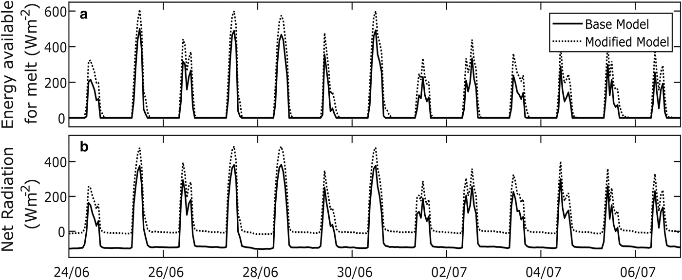
Fig. 9. Modeling results for the base and modified models for the cells at the glacier margin, with (a) the average energy available for melt and (b) the cells average net radiation.
Overall, Figure 9 shows that cumulated on the length of the experiment, the extra energy for melt computed by the modified model compared with the base model reaches 37.4 ± 5.6 × 10⁶ W m−2 with a 15% uncertainty value based on Machguth and others (Reference Machguth, Purves, Oerlemans, Hoelzle and Paul2008), who suggest an uncertainty for cumulative mass-balance modeling of 10%. Considering this estimate conservative, we use a value of 15% to calculate our uncertainties. Using a latent heat of fusion of 333.6 J g−1 and an ice density of 920 kg m−1, this cumulated extra energy for melt corresponds to 12.2 ± 1.8 cm of ice ablation for the margin cells. For the length of the dry season, from May to October, this value represents an extra ablation of 1.7 ± 0.3 m at the glacier margin compared with a simulation where the LW margin flux is not accounted for. However, this extra seasonal ablation should be considered as a first estimate because the LW margin flux is likely to vary throughout the season.
In terms of volume, the modified model computes an extra melt volume of 1361 m3 w.e. at the glacier margin over the 14 day simulation period. Because only one of the two glacier tongues was simulated with the LW margin flux, and because both tongues have a comparable length of ablation area margin (Fig. 1), it is hypothesized that the extra melt caused by the longwave margin flux for the entire glacier margin would be approximately doubled. The resulting 2722 ± 229 m3 w.e., the extra melt from the inclusion of the margin longwave flux, represents an increase of 2.7 ± 0.2% of the total glacier melt simulated by the base model over 14 days.
4. DISCUSSION
4.1. LW margin flux influence on tropical glaciers ablations
This study is a first attempt at quantifying the energy transfer happening at the glacier margins and its effects on ablation for tropical glaciers. We calculate an order of magnitude estimate for both important parameters and show that the longwave margin flux is a significant energy input for the ablation pattern at the glacier margin. Based on our results, this local energy flux should be considered as partly responsible for the strong lateral retreat pattern seen on tropical glaciers.
Moreover, as tropical glacier retreat, the ratio of glacier margin to ablation zone should increase, which will enhance the importance of the margin processes in a positive feedback. The feedback would only occur as long as the glacier margin has a steep slope angle or is adjacent to steep topography, which is likely as glacier margin ice cliffs have been known to maintain a steep slope angle and to persist over multiple years (Reid and Brock, Reference Reid and Brock2014).
It is likely that other local processes, such as warm air advection, are also factors resulting in enhancing melt at the margin. The calculations and results presented here for the longwave margin flux, based on distributed surface temperature measurements, should be considered as one plausible explanation to this retreat pattern and not as a complete picture of the physical processes happening at the glacier margin.
4.2. Comparison with ice-cliff backwasting
No literature was found that studied specifically the impact of longwave radiation from adjacent terrain to a glacier margin of a tropical glacier, but a useful comparison can be made with the study of ice-cliff backwasting on debris-covered glaciers. Our results on the importance of the margin longwave flux at the glacier edge are consistent with the result from Steiner and others (Reference Steiner2015). Steiner used a point-model of ice cliff backwasting on the debris-covered Lirung Glacier in the Himalayas and found that the longwave flux emitted by the adjacent debris to the ice surface was a significant input to the melt and compensated the deficit between incoming longwave radiation from the atmosphere and outgoing longwave emissions from the ice. The longwave flux from the debris calculated in his study ranges from 40 to 100 W m−2 depending on the season. Also on Lirung Glacier, Buri and others (Reference Buri, Pellicciotti, Steiner, Miles and Immerzeel2016) used a fully-distributed, grid-based model to calculate a mean hourly debris longwave flux of 70–80 W m−2, varying on the cliff and on the season and contributed to ~25% of the incoming longwave at the ice cliff. Both of these findings are in the same order of magnitude as the margin longwave flux calculated in this study, which varies from 80 to 120 W m−2 and contributes to 29% of the incoming longwave radiation at the glacier margin.
A comparison of the contribution to glacier-wide melt from ice-cliff backwasting and from the margin longwave flux is more difficult. The backwasting studies have focused on debris-covered glaciers, which show less surface ablation than a glacier with an exposed ice surface and therefore will have a higher proportion of their total ablation coming from exposed ice cliffs. Moreover, the studied glaciers are in different climate regions than our study in the tropical Andes. In the Alps, Reid and Brock (Reference Reid and Brock2014) found that the ice cliffs on the Miage Glacier accounted for 1.3% of the studied area, but contributed a disproportionate 7.4% of the ablation. At the Lirung Glacier, ice cliff backwasting for the two studied cliffs account for 0.02 and 0.07% of the studied area but contribute to 0.27 and 0.96% of the total melt. In the approach used in this study, we only calculate the increase in melt due to margin longwave flux and find that 0.3% of the glacier area is affected by the margin longwave flux, and this contributes to an overall melt increase of 2.7%.
4.3. Glacier margin geometry
An important parameter for our study is the glacier margin geometry. The margin geometry is one of the main factors determining the glacier view factors, and thus the magnitude of the energy transfer from the adjacent terrain to the glacier. For our study, the glacier margin geometry was assumed to be consistent along the studied ablation area. This allowed us to use the simplification of constant glacier view factors. However, glacier geometry will vary from glacier to glacier, and can also change along the margin of an individual glacier. To assess for what type of margin geometry the longwave margin flux is the most important, we use a simple sensitivity analysis of the impact of the glacier wall angle on the glacier view factor. The lower the angle of the glacier wall, the shorter the area of influence from the adjacent ground surface (Fig. 10). For a wall angle of 90°, the 15 m next to the margin will contribute to the longwave flux, with 42% of the longwave radiation emitted next to the glacier reaching the glacier wall. However, for a wall at 30°, only the first 5 m adjacent to the glacier will contribute to the margin longwave flux. For a margin angle of only 15°, the view factor immediately adjacent to the ice margin is already at 0.01. In this case, the emission from the ground adjacent to the glacier will not reach the glacier. The sensitivity analysis considered a changing glacier wall angle on a flat surface, but the same process would happen with a changing ground surface angle. A glacier margin facing a short cliff band or a rising pile of debris would have a high view factor as well. The one situation where the view factors do not allow for a longwave transfer is when the glacier lies at a very shallow angle (15° or less) to the ground surface. For any other glacier margin geometry, there will be a strong influence from the adjacent terrain contributing to the energy and mass balance at the glacier margin.
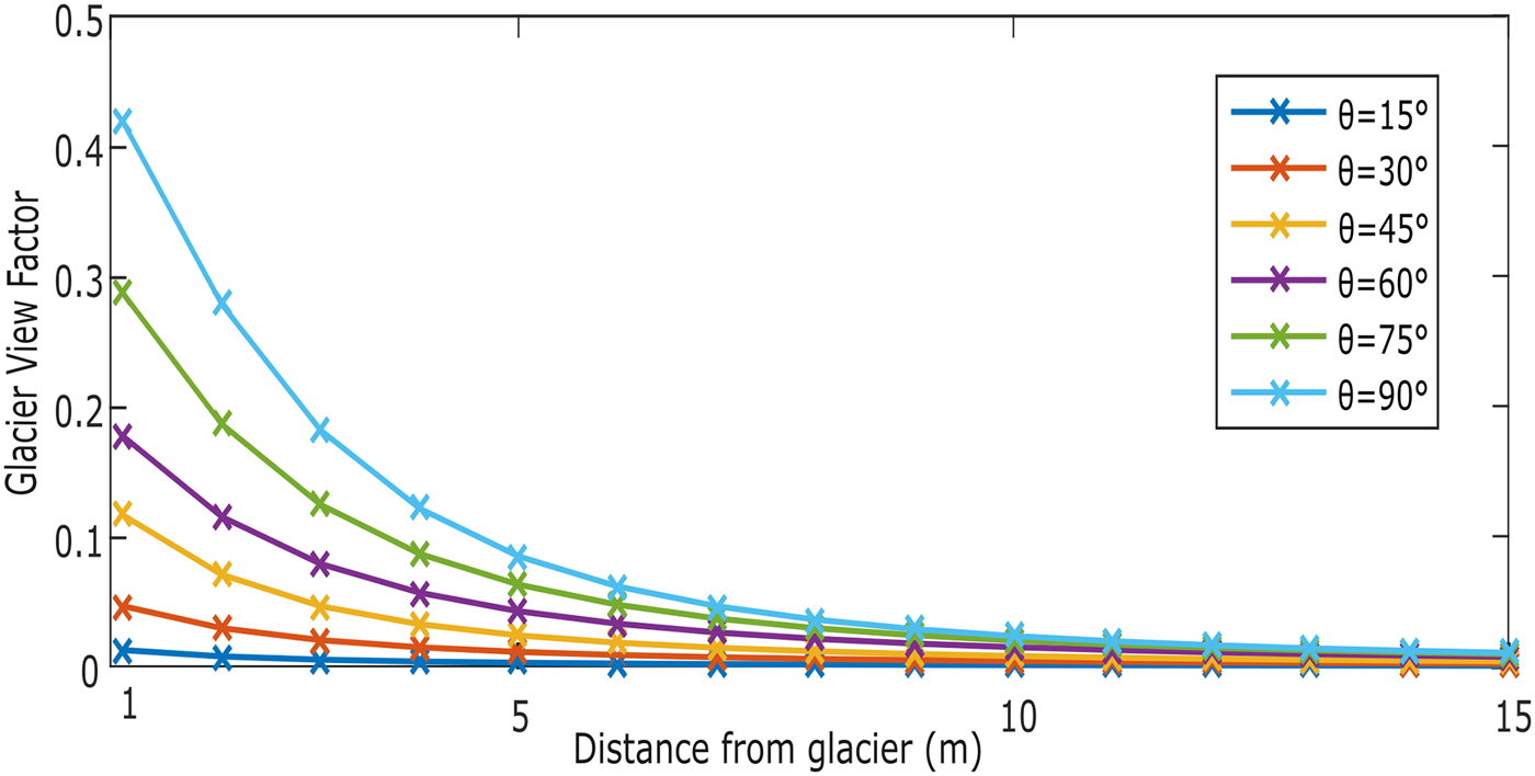
Fig. 10. View factors for different wall angles θ. In this study, the 75° (green) wall angle is used. A view factor threshold of 0.01 (dashed line) was used to defined areas contributing to margin longwave radiation.
4.4. Model uncertainty
The ablation estimations used in this study are based on a physically based energy-balance model designed not to require calibration for setting parameters. The model evaluation (Sections 3.5.1 and 3.5.2) shows that the model adequately reproduces measured ablation. Moreover, the model's outputs are being used for inter-comparison and are well adapted for the study objectives.
By targeting the main physical processes triggering melt, the model used in this study omits some other processes that may affect its accuracy without affecting significantly its outputs. First, the model does not distinguish directly between direct and diffuse shortwave radiation. When the topography obstructs the direct sunlight, incoming solar radiation to the shaded model cells is set to 15% of the calculated value without the shading to account for diffuse radiation. This simplification is justified by the assumption that, in our study, the impact of topographic shading on a glacier surrounded by high mountain peaks is more important than the impact of diffused shortwave radiation. In the tropical high Andes during the dry season, with the low relative humidity and the predominantly clear sky, filtering and scattering effects are minimal due to the thin air and the contribution from diffuse sky shortwave radiation is small (Benn and Evans, Reference Benn and Evans2010). The reflected terrain shortwave radiation, another component of diffuse radiation, is considered negligible as the surrounding mountains are composed of dark rock with no snow cover and high sky view factors (Gurgiser and others, Reference Gurgiser, Mölg, Nicholson and Kaser2013a). The importance of topographic shading on incoming solar radiation has been shown in multiple studies. Arnold and others (Reference Arnold, Willis, Sharp, Richards and Lawson1996) found that excluding shading increased incoming shortwave radiation by 5.8% for the Haut Glacier D'Arolla in Switzerland and resulted in an over-prediction of melt in high mountain environment and Brock and others (Reference Brock, Mihalcea, Kirkbride, Diolaiuti, Cutler and Smiraglia2010) found a reduction of incoming shortwave of 15% due to topographic shading on the Miage Glacier in Italy.
Second, the model does not account for topographic longwave irradiance from the surrounding mountains, which Plüss and Ohmura (Reference Plüss and Ohmura1997) estimated can cause an error up to 60 W m−2 when compared to unobstructed skies and Jiskoot and Mueller (Reference Jiskoot and Mueller2012) found an increase of 75–90 W m−2 from terrain radiation. However, including topographic incoming longwave radiation would be associated by a decrease in the incoming sky longwave, as some of the sky view factors would be obstructed. However, as relative changes in between the base and modified model only are used as modeling outputs, these factors do not significantly impact the results.
A sensitivity analysis is used to evaluate the effect of incoming shortwave radiation, incoming longwave radiation and albedo on model results. The sensitivity analysis is a common modeling technique that allows for comparison of parameter error on model outcomes (Somers and others, Reference Somers2016). The base model was run six times – twice for each of the three parameters that were varied by −10.0 and +10.0%, with the incoming shortwave radiation capped at the solar constant. The results are expressed as a percent change from the original base case simulation (Table 1). The results show that the model is most sensitive to the parameterization of the incoming shortwave radiation, with a 20.0% increase in glacial melt generation due to a 10.0% increase in shortwave radiation. The model was essentially equally sensitive to longwave radiation and albedo. Considering that incoming shortwave radiation is the main driver of melt for tropical glaciers, this result is not out of the ordinary, and reflects the sensitivity of the model to this critical parameter.
Table 1. The sensitivity of the base glacier melt model to the following parameters: incoming shortwave radiation, SW in , incoming longwave radiation, LW in and albedo parametrization
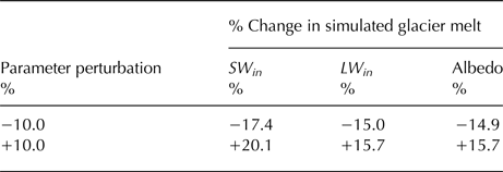
The values are percentage change of the simulated cumulative glacier melt for the 14-day base model run for each pertubation compared with the base model run result of 10.2 × 10⁵ m3.
The limited length of time of the simulations, coupled with the different assumptions made for modeling LW margin flux related processes, requires that care should be taken in interpretation of the results. The results provide an order of magnitude of the LW margin effects. The simulations show how margin ablation processes can be important in tropical glaciers and indicate the potential need for more margin radiation flux oriented model developments. These developments could include longer measurements of radiation fluxes at the glacier margin, to understand better the seasonality of such flux, a better representation of the glacier margin geometry to account for local topographic variations and more sophisticated melt models.
5. CONCLUSION
In this study, we used ground-based thermal infrared imagery to obtain a margin longwave radiation flux, emitted from the terrain surrounding the glacier. This flux varies between 80 and 120 W m−2 diurnally and is more dependent on local shading than on elevation. We include this margin longwave flux in a physically-based melt model of the glacier to investigate the impact on local ablation and energy balance at the glacier margin. The simulations show that the margin longwave flux has a visible impact on the net radiation and the available energy for melt at the glacier margins, increasing the energy available for melt by an average of 106 W m−2 during the daytime. The addition of the longwave margin flux also results in a net radiation that averages −6 W m−2 at night instead of −90 W m−2. The modified model shows an additional 2722 ± 229 m3 w.e. of melt over the 14-day study period, which is equivalent to an increase in melt of 2.7 ± 0.2% compared with the base model, generated by 0.3% of the total glacier area.
We present a previously unquantified energy flux affecting the energy balance at the glacier margin of a Peruvian glacier. This longwave flux from the terrain adjacent to the glacier, which for the 14-day study period amounts to an additional 12.2 cm of ice backwasting, may potentially explain retreat patterns seen on some tropical glaciers, where accelerated mass loss is noticed not only at the lowest elevation along the glacier toe but along the entire margin of the ablation zone. As the glacier melts, the ratio of glacier margin to total area increases and the importance of the margin longwave flux derived in this study would increase. Therefore, even if this flux is not a significant input to glacier meltwater generation in this situation, it is potentially an important contribution to glacier retreat pattern.
To the best of our knowledge, this is the first quantitative assessment of the longwave energy transfer happening at the glacier margin of a tropical glacier. This significant energy flux should be investigated at more locations, with special attention given to the variation in margin geometry and the variation in view factors along the glacier margin. Moreover, a longer study period would be beneficial to obtain a more complete picture of the ablation pattern resulting from this longwave margin flux. More studies on this topic and the inclusion of the margin longwave energy flux into further melt modeling studies would improve the assessment of meltwater generation and ablation patterns for tropical glaciers.
With accelerated glacier loss worldwide, water resources for population downstream of glaciated terrain are threatened. This is especially true in regions with a precipitation deficit during part of the year, such as the Cordillera Blanca, Peru, where there is effectively no precipitation during the dry season (Baraer and others, Reference Baraer2012). This study provides valuable information to better understand the driving glacier ablation in tropical climates and predict future water availability in these already water-stressed areas.
SUPPLEMENTARY MATERIAL
The supplementary material for this article can be found at https://doi.org/10.1017/jog.2017.85
Acknowledgment
We thank Autoridad Nacional del Agua, in particular, the staff of the Huaraz Office, the Parque Nacional Huascarán and Jesus Gomez. We also thank Oliver Wigmore for providing the DEM of Cuchillacocha Glacier as well as James DeGrand for assisting with the instrumentation. We also thank Wolfgang Gurgiser and an anonymous reviewer whose comments greatly improved the paper. The project is supported by grants from NSERC, including the Research Tools and Instruments Program, and the National Science Foundation under grants EAR-1316429 and EAR-1316432. Additional thanks to McGill University and L'École de Technologie Supérieure de Montréal for additional support. Aubry-Wake received funding for a scholarship for Master's studies from The Fonds de recherche du Québec - Nature et technologies. Please contact the corresponding author for use of published data.


 Open access