


1 Introduction
Proper representation of the basal boundary condition of ice sheets is essential to evaluate their evolution, and to project how they will behave in the future. For contemporary ice sheets, it is possible to make a general inference on basal properties based on present day observations of velocity, bed topography and ice surface height (e.g. Joughin and others, Reference Joughin, MacAyeal and Tulaczyk2004; Shapero and others, Reference Shapero, Joughin, Poinar, Morlighem and Gillet-Chaulet2016), or through geophysical measurements (e.g. Anandakrishnan and Winberry, Reference Anandakrishnan and Winberry2004; Walter and others, Reference Walter, Chaput and Lüthi2014). The velocity of glaciers is influenced by seasonal variations in water reaching the base, which causes fluctuations during the melt season (Zwally and others, Reference Zwally2002; van de Wal and others, Reference van de Wal2008). An ice sheet model should be able to incorporate the presence of deforming sediments (Alley and others, Reference Alley, Blankenship, Bentley and Rooney1986) and hydrologically induced velocity changes (Clason and others, Reference Clason2015; de Fleurian, Reference de Fleurian2016).
Most actively developed ice sheet models incorporate a basal sliding law using the shallow shelf approximation (SSA) and the hypothesis that the bed is covered by deformable sediments (for instance PISM Bueler and Brown (Reference Bueler and Brown2009); Winkelmann and others (Reference Winkelmann2011); PISM authors (2022)), or a spatially varying basal traction constant in a Coulomb friction or power law sliding (for instance, BISICLES (Cornford and others, Reference Cornford2013), SICOPOLIS (Bernales and others, Reference Bernales, Rogozhina, Greve and Thomas2017), Elmer/Ice (Gagliardini and others, Reference Gagliardini, Cohen, Råback and Zwinger2007, Reference Gagliardini2013), ISSM (Morlighem and others, Reference Morlighem2010), and CISM (Lipscomb and others, Reference Lipscomb2019)). Elmer/Ice, ISSM and SICOPOLIS also have models that couple the subglacial hydrology to the basal conditions (Gagliardini and Werder, Reference Gagliardini and Werder2018; Smith-Johnsen and others, Reference Smith-Johnsen, de Fleurian and Nisancioglu2020; Goelzer and others, Reference Goelzer2020; Greve and others, Reference Greve, Chambers and Calov2020). These models were generally developed for use within the existing Greenland and Antarctic ice sheets, where details on the nature of basal conditions are limited. Earlier ice sheet models using simpler ice flow approximations demonstrated the importance of hydrology on ice sheet evolution (Arnold and Sharp, Reference Arnold and Sharp2002; Clason and others, Reference Clason, Applegate and Holmlund2014).
At present, there is no open source ice sheet model that couples seasonally changing hydrological conditions, and basal conditions that include changes in sediment cover, while using the more advanced ice flow physics in a way that can be applied to the 100 000 year time scales of continental glaciation. For the North American and Eurasian ice sheets, although we know about the distribution of sediments and can make inferences on ice sheet flow based on landforms (Stokes and Clark, Reference Stokes and Clark2001; Margold and others, Reference Margold, Stokes and Clark2015; Greenwood and others, Reference Greenwood, Clason, Nyberg, Jakobsson and Holmlund2017), the constants used in the sliding laws used in ice sheet models have no reference ice thickness or velocity field in which to tune them. Therefore, it is desirable to create a model that can utilize observations from surficial geology and geomorphology to control the parameterization of glacial sliding.
We present a new basal condition model within the Parallel Ice Sheet Model 1.0 (PISM) (Bueler and Brown, Reference Bueler and Brown2009; Winkelmann and others, Reference Winkelmann2011; PISM authors, 2022) that incorporates these features. Our intent is to create a model that provides more realistic basal boundary conditions, while still being efficient enough to run on glacial time scales. Prior to this, PISM did not have a way to couple surface meltwater to the basal sliding model, nor did it have a way to incorporate sliding without sediment deformation. Our model is computationally inexpensive, even over a continental size domain, and is therefore suitable for simulating paleo ice sheets. We provide a suite of tests of the variables available within the model, and provide recommendations on usage. Finally, we apply the model to the North American continent to simulate the Cordilleran and Laurentide ice sheets, to show how the change in basal conditions can affect ice sheet growth and retreat.
2 Methods
2.1 Hydrology model
The hydrology model is based on the concept that a certain amount of water gets stored in the sediments underlying the ice sheets, and, once saturated, the excess is transported in the direction of the hydrological gradient to the ice margin. Some components of our model derive from the routing scheme described by Bueler and van Pelt (Reference Bueler and van Pelt2015), but we have simplified the implementation to emphasize computation speed. Our model does not conserve mass, and transports water to the edge of the ice sheet without any time delay. When the routing of the excess water is computed, the water from upstream grid cells is added to each grid cell downstream. This is not entirely realistic, since the hydrological system can react at a time scale on the order of hours (Bartholomew and others, Reference Bartholomew2012). The time stepping in the model is usually on the order of days to months, so this simplification may be considered to be representative of average conditions. Ultimately, the output of the hydrology model is the effective pressure at the base of the ice sheet, which is then transferred into the basal sliding model. A schematic of the components of our model is shown on Figure 1, while Figure 2 shows the workflow of the model.
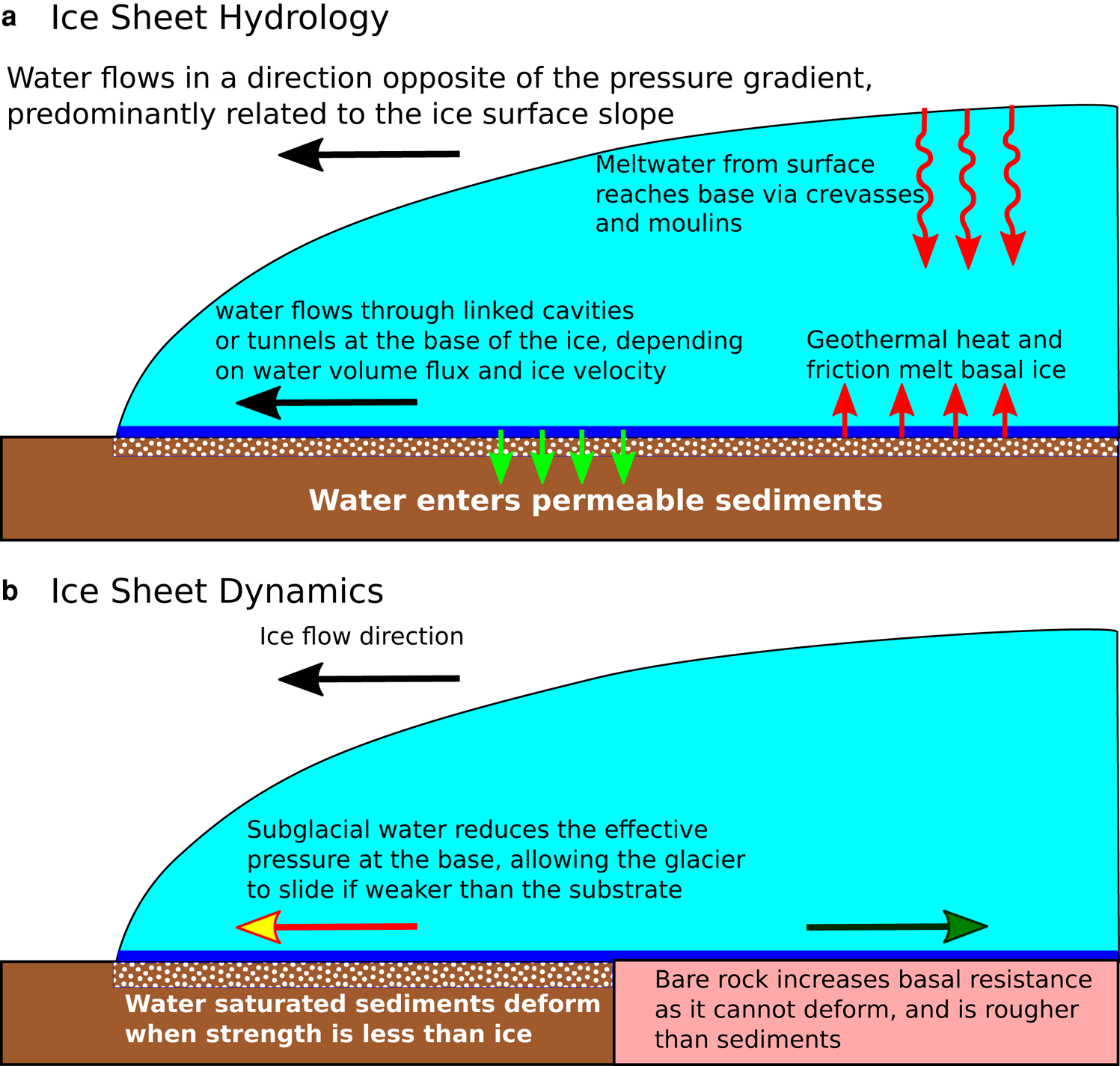
Fig. 1. Schematic of the components of the new basal conditions model. (a) Overview of ice sheet hydrology. (b) Overview of impact on sliding.
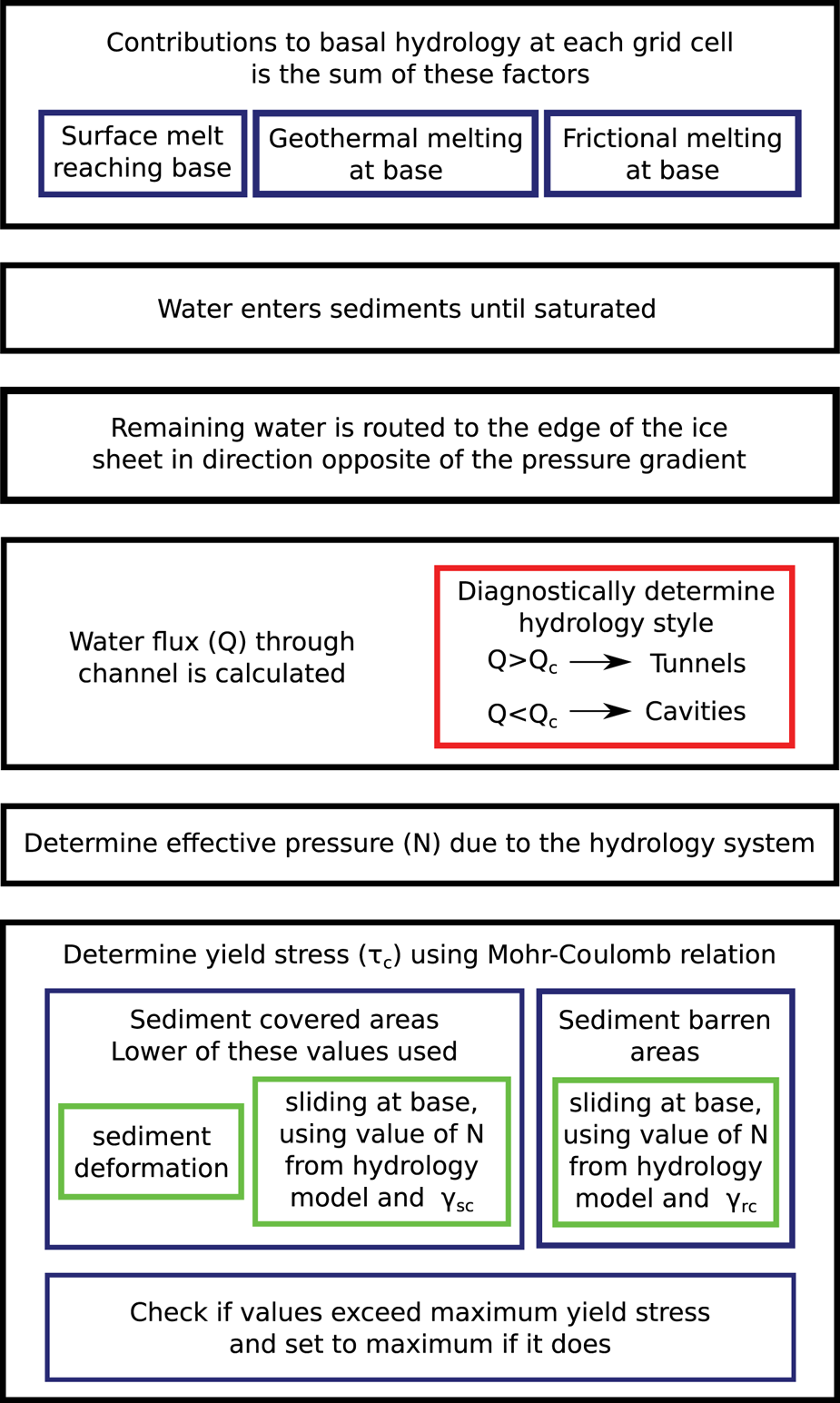
Fig. 2. Diagram showing the workflow of the model.
2.1.1 Water routing
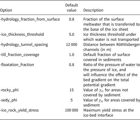
The first component of the model is that it captures the surface melt. We are using the semi-analytical positive degree day (PDD) method module (Calov and Greve, Reference Calov and Greve2005). As implemented in PISM, it computes the amount of ice that melts at the surface as a diagnostic parameter. Our modification stores this value and passes it to our hydrology model. Within our model, there is an option to set the fraction of the meltwater that gets transferred to the base of the ice sheet (see Table 1 for a full list of command line options available for the model). The water transferred from the surface is added to the meltwater generated from heating at the base (Aschwanden and others, Reference Aschwanden, Bueler, Khroulev and Blatter2012).
Table 1. Command line options available for the described models
The next step is a modification of the undrained plastic bed model (Tulaczyk and others, Reference Tulaczyk, Kamb and Engelhardt2000; Bueler and Brown, Reference Bueler and Brown2009). In this model, a layer of sediment of a specified thickness and porosity fills with water until it is saturated, which is set within PISM as a ‘water thickness’ parameter, W sed. The saturation, s, is:

W sed is the amount of water in the sediments, represented as a layer below of the ice sheet that fills when there is water input into the subglacial hydrology system, while $W_{sed}^{\max }$ is the maximum thickness of that layer. In our simulations, $W_{sed}^{\max } = 1$
 m, the value used in Niu and others (Reference Niu, Lohmann, Hinck, Gowan and Krebs-Kanzow2019). If the porosity of a deforming till is 40% (Blankenship and others, Reference Blankenship, Bentley, Rooney and Alley1987), this value implies that 2.5 m layer of subglacial sediment is active in the hydrology system of the ice sheet.
A certain amount of accumulated water within the sediment is removed at every time step in order to simulate drainage. This is determined by reducing the basal water layer thickness at a rate of 1 mm yr−1, which is the default value in PISM. At every grid cell where s < 1, any subglacial water will be added to the sediments. Our modification from the default model is that the amount of water that can enter the sediments depends on the fraction of the subglacial surface that is covered in sediment. If the sediment cover is incomplete, then the sediments can fill with water to the maximum level faster than if there is complete cover since there is less sediment to accommodate the water. Note that our model does not take into account the possibility that the underlying sediments are impenetrable due to being frozen. The consequence of this is that the water flux is underestimated (since water would not be able to enter the sediments) and the area where sediment deformation happens would be overestimated (since frozen sediments cannot deform).
Any excess water in the grid cell after filling the sediments is transported to the edge of the ice sheet. We use a simple subglacial water routing routine, where the water is transported in the direction opposite to the hydrological potential gradient, $\nabla \phi _h$ . Note that the routing of water happens after the sediment filling step, so none of the water added to a grid cell from upstream contributes to the water in the sediments. The equation for calculating the potential gradient at the base of the ice sheet is as in Cuffey and Paterson (Reference Cuffey and Paterson2010):
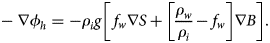
In this equation, ρ i is the ice density, ρ w is the water density, g is the gravitational acceleration, $\nabla S$ is the ice surface gradient, $\nabla B$
 is the bed gradient, and f w is the flotation fraction, which is the ratio of the water pressure and overburden pressure. The flotation fraction governs the relative influence of the bed and ice surface slopes on the direction of water flow. We have set it to be a constant, f w = 0.8, which gives the surface slope a 2.7 times greater influence on the routing (Cuffey and Paterson, Reference Cuffey and Paterson2010). This ensures that the water will generally move toward the edge of the ice sheet. We calculate the gradient either using a third order finite difference method described in Skidmore (Reference Skidmore1989) or using a least squares method on a 5 × 5 grid (i.e. all the grid cells within 2 cells of cell where the gradient is calculated), the later which is the default.
The routing of water is accomplished by first sorting the hydrological potential, ϕ h, values over the entire grid from highest to lowest. In order to avoid singularities, S and B are smoothed using a 5 × 5 average filter. The potential values are sorted from highest to lowest and the water is routed in the direction opposite to the gradient. This results in increasing amounts of water toward the edge of the ice sheet, where the potential will be the lowest as the ice sheet is thinnest. If the gradient of a cell is below a certain threshold (which we have set to be 1.0 N m−3), then no water is distributed as it is assumed that the water would be flowing too slowly to be distributed. The amount of water determined to go through each grid cell, which we define as T w, is used to determine the effective pressure, which is described in the next step. The amount of water, T w is expressed as the thickness of water over the entire grid cell per unit time (i.e. units of m s−1).
2.1.2 Effective pressure
To calculate the effective pressure, we use a parameterization described by Schoof (Reference Schoof2010). This parameterization is based on the concept of water drainage at the bottom of the ice sheet being routed through efficient Röthlisberger channels (Röthlisberger, Reference Röthlisberger1972) or less efficient linked cavities (Kamb, Reference Kamb1987). This is a modification of other subglacial drainage models that have been proposed in the past (Fowler, Reference Fowler1987; Hewitt and Fowler, Reference Hewitt and Fowler2008), but allows for better switching between drainage styles. The style of drainage system is dependent on the amount of water available and the velocity of the ice. In this formulation, the effective pressure decreases up to a certain point, after which drainage becomes efficient enough that it causes the effective pressure to increase again.
The main component of this model is the switch between channel and cavity drainage systems. The type of drainage system is dependent on the total water flux, Q. The threshold water flux, Q c is calculated by the following equation:
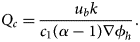
The velocity of the ice at the base is u b. In this model, the bed is assumed to be rough, with a protrusion height of k, which we have set to be 0.1 m. The constant c 1 is related to the latent heat of fusion of ice, L, and is calculated by c 1 = 1/(ρ i L). The constant α = 5/4 is related to the Darcy–Weisbach equation friction factor for water flow in a conduit (Schoof, Reference Schoof2010). This quantity is calculated purely as a diagnostic value, and does not influence the modeled drainage system.
For the parameterization from Schoof (Reference Schoof2010), the effective pressure is calculated using the assumption that the water discharge is in steady state. This assumption reduces the complexity of the effective pressure calculation, since it does not have dependence on the size of the conduits or the style of drainage system. We use the total amount of water going through each cell, T w, as calculated in the previous section, to determine the water flux. The water is assumed to be directed through a single channel. The total flux of water through a channel, Q, considering a grid cell of width dx is calculated as follows:

The value of r is the spacing between channels. This value is set to a constant of 12 km, which is the average distance between eskers on the Canadian Shield (Storrar and others, Reference Storrar, Stokes and Evans2014). This formulation allows for the proper parameterization of water flux through the channel regardless of the actual width of the grid cell. Based on Eq. (3), if Q > Q c, then the routing is via the tunnel system (efficient drainage), while if Q < Q c, the drainage is via a cavity system (inefficient drainage). As a result of this formulation, if the ice velocity increases, the threshold amount of discharge to switch to efficient tunnel drainage also increases.
The effective pressure in the drainage system, N hyd is calculated by the following equation (Schoof, Reference Schoof2010):
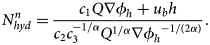
The exponent, n is the Glen exponent, which by default is 3. The thickness of the ice is h. The velocity of the ice at the base is u b. The constant c 2 = 2 A n −n includes parameters in Glen's law, where A is the ice softness. The default value is A = 3.1689 × 1024 Pa−3 s−1 (Huybrechts and Payne, Reference Huybrechts and Payne1996). The constant c 3 is related to the relation for turbulent flow of water in the Darcy–Weisbach equation, where $c_3 = 2^{1/4} \sqrt {\pi + 2} / [ \pi ^{1/4} \sqrt {\rho _w f}]$ , and f is a friction factor. We use the value f = 0.1 (Schoof, Reference Schoof2010).
There is a check so that the calculated effective pressure is not greater than the overburden pressure:

If the effective pressure is greater than the threshold, it is set to be equal to the overburden pressure. This can happen if the water flux, Q, becomes much smaller than u b h. There is also a check to ensure that the effective pressure is greater than a minimum threshold, which we have set to be 0.01 times the overburden pressure. This should rarely happen except if the equation is solved where there is essentially no ice, or where there is no surface gradient and velocity. In reality, negative effective pressures can exist under glaciers when there is a rapid influx of water, which can cause the ice to temporarily float (Roberts, Reference Roberts2005). Here we have removed the possibility of negative effective pressure only to ensure the stability of the ice sheet model.
2.2 Basal sliding model
The sliding model that we use is basically a modification of the existing Mohr–Coulomb yield stress relationship that is generally used as the sliding law in PISM (Bueler and van Pelt, Reference Bueler and van Pelt2015). The general definition for the Mohr–Coulomb yield stress, τ c, is a function of the effective pressure, N, the angle of internal friction, ϕ, and a cohesion parameter, c.
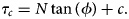
The value of ϕ determines the angle that the material will fail if a normal stress is applied. In the default PISM sliding law, the entire base of the ice sheet is assumed to be covered in a layer of deformable sediments (i.e. soft bedded sliding), and ϕ is the shear friction angle of the sediments. For sediments, this value will depend on the dominant grain size, with clay materials having a lower value than sand and gravel. When a sediment under the ice sheet becomes water saturated, the effective pressure decreases, which increases the chance of failure. In general, the cohesion is regarded as being negligible in a deforming till (Cuffey and Paterson, Reference Cuffey and Paterson2010), so it is set to c = 0.
In PISM, the basal shear stress, τ b that balances the driving stress is related to the yield stress τ c by (Bueler and Brown, Reference Bueler and Brown2009):
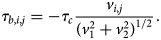
In this equation, v is the basal ice velocity, and the indices i, j refer to the directional components of the velocity. In PISM, the SSA is used to compute the stress balance only when v > 0, otherwise the non-sliding shallow ice approximation (SIA) is used. The value of τ c used in the modified model is described below.
The modified sliding law has two components, sliding due to the deformation of saturated sediments, and sliding due to the interactions between the water in the drainage system and the ice-bed interface. The sliding between the ice and the substrate when the effective pressure is low due to high water pressures is considered to be analogous to a landslide, and can also be described using the Mohr–Coulomb relationship (Cuffey and Paterson, Reference Cuffey and Paterson2010). The PISM module we have created solves for both of these sliding mechanisms, and will chose the one that has a lower yield stress.
Our modified sliding law allows for spatially variable sediment cover, as places such as the Canadian Shield in North America did not have complete sediment cover (i.e. hard bedded sliding) (Fulton, Reference Fulton1995). This sliding law still allows for sediment deformation as utilized in the default PISM sliding law, and for sliding at the ice-bed interface. In this sliding law, the strength of the bed is calculated for both sediment deformation and sliding along the bed-ice interface, and the lower value is used.
First, we describe the yield stress due only to sediment deformation. The fraction of the area that is covered in sediment, S f, can be spatially variable. This affects both components of the basal sliding model. For areas that have incomplete sediment cover, sediment deformation only happens for the fraction of the surface that has sediment, while the rest of the area is set to have a yield stress that is equal a user adjustable value, τ bare (by default it is set to 100 kPa, which is a typical value of the yield stress at the base of a glacier (Cuffey and Paterson, Reference Cuffey and Paterson2010)). In reality this value will depend on factors such as the roughness of the bed, the debris content of the ice, and temperature, all factors that we do not estimate. This value is also set to be the maximum yield stress in sediment covered areas. The overall yield stress, τ def, is:

where τ sed = N sedtan (ϕ sed) is the yield stress of the sediments. The result of this is that areas with incomplete sediment cover will be less likely to be influenced by sediment deformation as the primary mode of sliding. We sometimes refer to S f as the percentage cover, although in these equations and in the code, it is expressed as a fraction. The effective pressure in the sediments, N sed is the same as described by Bueler and van Pelt (Reference Bueler and van Pelt2015):

This equation has several constants, which in PISM are derived from Tulaczyk and others (Reference Tulaczyk, Kamb and Engelhardt2000). N o = 1000 Pa is the reference effective pressure. e 0 = 0.69 is the void ratio at the reference pressure. C c = 0.12 is the compressibility of the sediments, which for this value refers to glacial till. P o is the overburden pressure. The value s is the water saturation of the sediments, which is taken from the hydrology model described above.
For the second component of the sliding law with sliding along the ice-bed interface, the Mohr–Coulomb relationship is also used. In this case the ϕ value is related to the roughness of the interface between the ice and the bed (Iken, Reference Iken1981; Cuffey and Paterson, Reference Cuffey and Paterson2010). For clarity, we define the angle in this component as γ. A Coulomb-style law has been found to be sufficient to describe hard bedded sliding (Helanow and others, Reference Helanow, Iverson, Woodard and Zoet2021). In this model, the base of the ice sheet is covered by bumps, with an upslope angle that is equal to γ. There is a separate value for sediment covered areas (γ sc) and areas where the bed is rock (γ rc), as it is assumed that sediment covered areas will be smoother. First the model checks if the yield stress over sediment covered areas, N hydtanγ sc, is lower than the value from sediment deformation, N sedtanϕ sed. This lower value is taken as the yield stress over sediment covered areas and denoted as τ sedfrac.

As a result, if sediment cover is almost complete and the sediments are saturated with water, the effective yield stress will be similar to the default sliding law of PISM. The overall yield stress, τ slide is:

The values of γ for sediment covered and bare areas can be set by the user. The effective pressure, N hyd, is taken from the hydrology submodel described in the previous section.
After the yield stress for both sediment deformation and sliding at the base has been calculated, the lower of the two values is chosen as the yield stress for calculating sliding.

In addition to sediment deformation and the combined hydrology and sediment deformation methods to find the yield stress, there is also an optional method to artificially impose a low value at the grounding line of the ice sheet when it is beside an ice shelf (the option is called ‘slippery grounding lines’ – sgl). The slippery grounding line option will ensure that the sediments are completely saturated. There is also an additional value of the potential yield stress, τ sgl calculated, which scales the overburden pressure using the following relationship:

where b is the elevation, g is the gravitational acceleration and ρ i is the density of ice. These equations scale the yield stress to be 0.1 to 0.2 times the overburden pressure above −1000 m, between 0.1 and 0.001 times the overburden pressure between −1000 and −2000 m, and 0.001 times the overburden pressure lower than −2000 m. This scaling will allow a reduction in the yield stress at the grounding line even where there is incomplete sediment coverage. The value of τ sgl is used if it is lower than τ slide and τ def.
2.3 Limitations
In reality, if there was enough water under the ice sheet, it would cause the ice sheet to float (i.e. the water pressure would exceed the overburden pressure and N hyd would be negative) (Schoof and others, Reference Schoof, Hewitt and Werder2012). The model does not take into account this possibility, and as a result limits the seasonal acceleration of the ice sheet. Another issue is the lack of water storage underneath the ice sheet. If there is a localized hydrological potential low point within the ice sheet, water would be routed toward this point. If enough water were to collect at such a point, it is likely that a subglacial lake would form. Since the influence of bed topography is reduced using the variable f w, this problem is reduced, as the ice surface generally decreases toward the edge of the ice sheet. A future addition to this model that would make it more realistic would be to incorporate water conservation between time steps. This could be used to determine if a subglacial lake would form. The consequence of these limitations is that the modeled velocity of the ice sheet will be slower than reality, as a subglacial lake would essentially remove the resistance to flow at the base (Thoma and others, Reference Thoma, Grosfeld, Mayer and Pattyn2012). As an example, the ice velocity over a well studied subglacial lake in the Whillans and Mercer ice streams in Antarctica increased by up to 4% when it filled (Siegfried and others, Reference Siegfried, Fricker, Carter and Tulaczyk2016).
Our model does not take into account the possibility of spatially variable sediment thickness beyond having the possibility of having sediment free areas. This is not seen as being a major limitation, because sediment deformation mostly happens in the uppermost one meter of sediment (Boulton and others, Reference Boulton, Dobbie and Zatsepin2001). A larger possible consequence would be on the volume of water that could be stored subglacially in the sediments. Given the time scales of glacial cycle models, we regard this as a minor issue, as we expect that the aquifers would remain close to being full if water was consistently reaching the bed.
The effective pressure calculation uses an assumption that the water flux is in steady state. The style of drainage is implicit in the equation, and does not evolve if the flux is no longer in steady state. In reality, the drainage system does not necessarily switch back to an earlier state if there is a reduction of flux (Schoof, Reference Schoof2010). A more accurate drainage model would require explicit determination of the evolution of the geometry of the channels or tunnels.
Another limitation is the spatial resolution of the model simulation. The way the model is set up, it is assumed that the water is distributed to the adjacent cells. In a higher resolution model run, the pathway the water takes may become more focused than in the coarser tests that we have run. This would result in some pathways having a much higher water flux, while some adjacent cells would be much lower. The increased influence of the hydrological component of the model would be competing against adjacent cells that might not undergo a seasonal reduction in yield stress.
3 Modeling
3.1 Model setup
We test our model using two experimental setups. The first is an idealized circular ice sheet with a strip that has differing basal conditions, in order to test the sensitivity to various parameters used in the model. The second is a glacial cycle simulation in the area covered by the Laurentide and Cordilleran ice sheets in North America. This tests the model in a more realistic setting, using spatially variable topography and sediment properties (Gowan and others, Reference Gowan, Niu, Knorr and Lohmann2019). In both cases, the model parameters used in this study are the same as used in Niu and others (Reference Niu, Lohmann, Hinck, Gowan and Krebs-Kanzow2019), except where noted. We briefly summarize the basic model setup here.
The stress balance of the ice sheet uses a combination of the SIA and SSA (Bueler and Brown, Reference Bueler and Brown2009). The surface mass balance is driven by the positive degree day method (Reeh, Reference Reeh1991). The precipitation and temperature fields are varied between two climate states using an index, as implemented by Niu and others (Reference Niu, Lohmann, Hinck, Gowan and Krebs-Kanzow2019). Marine-ice sheet interactions make use of the PISM-PIK parameterizations, which control the ice sheet behavior of ice shelves and the grounding line (Winkelmann and others, Reference Winkelmann2011; Albrecht and others, Reference Albrecht, Martin, Haseloff, Winkelmann and Levermann2011; Levermann and others, Reference Levermann2012).
For calving of floating ice shelves, we have modified the thickness calving scheme in PISM. The default version causes any floating ice less than h = 200 m to be calved. This might be appropriate for Antarctica, where the shelf edge floats over very deep water. However, in the shallow Hudson Bay, where tidal and wave driven stresses would be far less, this is not appropriate. In our initial experiments, this harsh calving criteria prevented the advance of the ice sheet into Hudson Bay. Our modified version changes the threshold thickness for calving, h ct, to be dependent on the water depth, b, and a scaling parameter c:

For our experiments, we use a value of c = 0.1. We also set minimum and maximum thresholds for the calving. The maximum threshold is h ct(max) = 200 m, which is the default value of the thickness calving module (i.e. at the calving front, the ice shelf will only calve when the thickness becomes less than 200 m even when cb > 200). The minimum threshold is h ct(min) = 40 m, which prevents the formation of very thin ice shelves (i.e. the ice shelf will always calve if below h ct(min), regardless of the value of cb). Any place where the floating ice is h < h ct is calved.
As we wish to test the impact of changing basal conditions in the context of terrestrially terminating ice sheets (as the southern and western margins of the Laurentide Ice Sheet were), we have chosen to use the purely elastic glacial isostatic adjustment (GIA) module in PISM. The Lingle-Clark model (Lingle and Clark, Reference Lingle and Clark1985; Bueler and others, Reference Bueler, Lingle and Brown2007) with a viscous half-space mantle that was used in Niu and others (Reference Niu, Lohmann, Hinck, Gowan and Krebs-Kanzow2019) has a tendency to produce unrealistically depressed basins when applied to the glaciation of the Laurentide Ice Sheet, likely the result of the lack of a contrasting high viscosity lower mantle. These basins are often below sea level, which PISM interprets as being ocean basins. This is not desirable in our experiments, and the elastic deformation model allows us to avoid this problem. In addition, we have kept sea level as a constant to avoid sea level induced fluctuations of the ice sheet (i.e. Gomez and others, Reference Gomez, Weber, Clark, Mitrovica and Han2020).
3.2 Idealized circular ice sheet experiments
3.2.1 Overview
In order to test the effects of our basal conditions model, we have created an idealized setup that produces a circular ice sheet if the basal conditions are uniform over the domain. The ice sheet is generated by interpolating between two different climate states (i.e. a glacial index), representing a glacial state and an ice free state. A circular ice sheet is achieved by setting the coldest conditions at the center of the domain, and increasing the temperature toward the edge of domain. The values for the temperature and precipitation at the center and edge of where the circular ice sheet form were derived from the glacial cycle simulations by Niu and others (Reference Niu, Lohmann and Gowan2019a). We use a sinusoidal index with a period of 40 000 years, so that the coldest conditions happen at 20 000 years. As noted by Niu and others (Reference Niu, Lohmann and Gowan2019a), the maximum size of the ice sheets in this kind of experiment happens after the minimum in coldness, in our case at about 25 000 years. This is the time that we chose to compare the results of the experiments, since the ice sheet was near the maximum growth, and the elevation differences at the edge of the ice sheet are not substantial between the experiments. At this point, the equilibrium line altitude for melt and accumulation is increasing, which causes meltwater to be produced at the surface. After 25 000 years, the surface height and margin location are different, because of the differing basal conditions, so the velocity cannot be easily compared. Figure 3 shows the general setup for the experiments, including the ice surface elevation and ice thickness near the edge of the ice sheet. Since there are changes in the basal conditions, this results in differing ice thickness evolution.
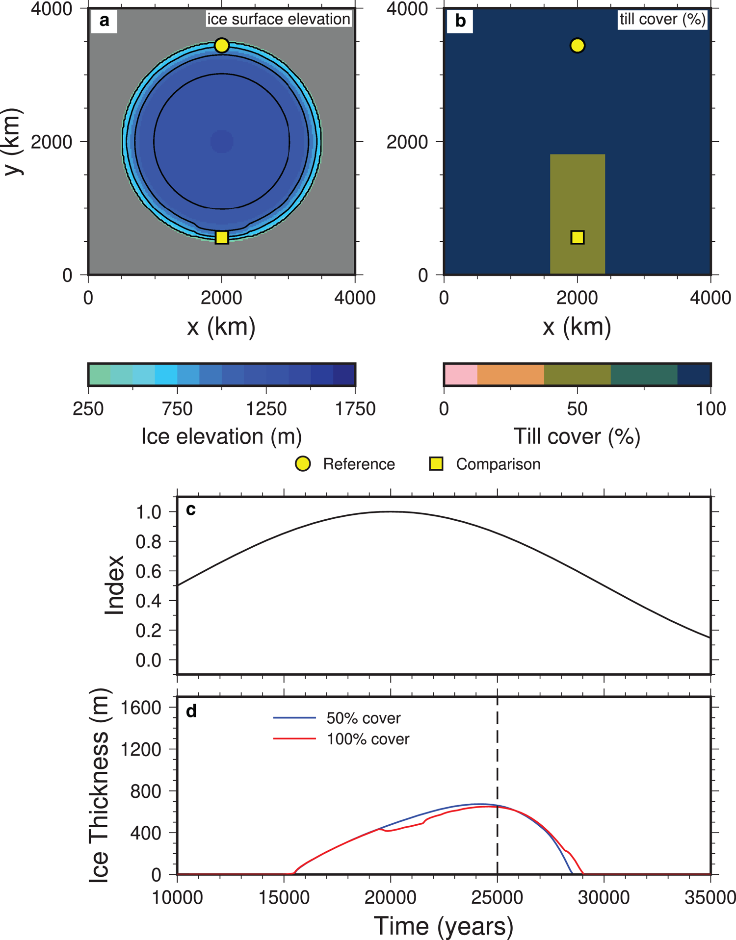
Fig. 3. Experiment with a strip of S f =50% sediment cover, with γ rc = 2° for areas with bare rock, and γ sc = 1° for areas covered in sediment. For sediment deformation, ϕ sed = 20°. The percentage of surface meltwater reaching the base is 80%. (a) Ice surface elevation at 25 000 years. (b) Sediment (till) cover fraction, showing the strip with reduced cover. Also shown are the locations that are used to compare the velocity and sliding properties. (c) Index used to linearly interpolate the climate variables, where 0 is warm conditions, while 1 is glacial conditions. (d) Ice thickness evolution at those two locations, showing a greater thickness in the partially covered strip, as the velocity is less.
Figure 4 shows a time series example demonstrating the switching between different hydrology types and sliding mechanisms for four idealized experiments (plots for all of the experiments can be found in the Supplementary Material). The velocity of the ice sheet at different points of the year for the experiment with $S_f = 50\percnt$ and $\phi _{sed} = 20^\circ$
 is shown on the left side of Fig 5. This particular experiment shows that there is a switch to an inefficient cavity system when water flux is introduced. The velocity increases during the summer, though it never reaches the value of the fully sediment covered areas. In the case with $\phi _{sed} = 30^\circ$
 , the ice sheet is able to achieve velocities comparable to the fully covered areas, as the velocity from sediment deformation is lower. When S f = 80% , there is still an increase in velocity during the summer, but the magnitude of the difference from the winter value is not as great. At the end of the melt season, the calculated effective pressure becomes higher than the overburden, triggering the limit described before. When the index is artificially changed to create a warmer climate (by using the 25 000 year ice sheet using the climate at 35 000 years), the higher surface meltwater production causes the drainage system to switch to a tunnel system, and causes a slight reduction in velocity. In this test, the velocity increases slightly at the end of the melt season when the hydrology system returns to the cavity system.

Fig. 4. Basal conditions and velocity time series for the locations shown in Figure 3 at about 25 000 years with S f values of 50% or 80% (blue lines) and 100% (red lines) and ϕ sed values of 20° and 30° and glacial index set to 25 000 years or 35 000 years. (a) Volume water flux, primarily from meltwater from the surface being transferred to the base. (b) Type of water routing at the base of the ice sheet that determines the effective pressure. ob - overburden, cav - cavities, tun - tunnels/channels, dry - no water in the system. (c) Sliding law method used by PISM. sgl - slippery grounding lines, slide - modified sliding law that takes into account both sediment deformation and sliding at the ice-bed interface, sed - sediment deformation only model (PISM default), none - no sliding (i.e. no ice is present). (d) Surface velocity magnitude.
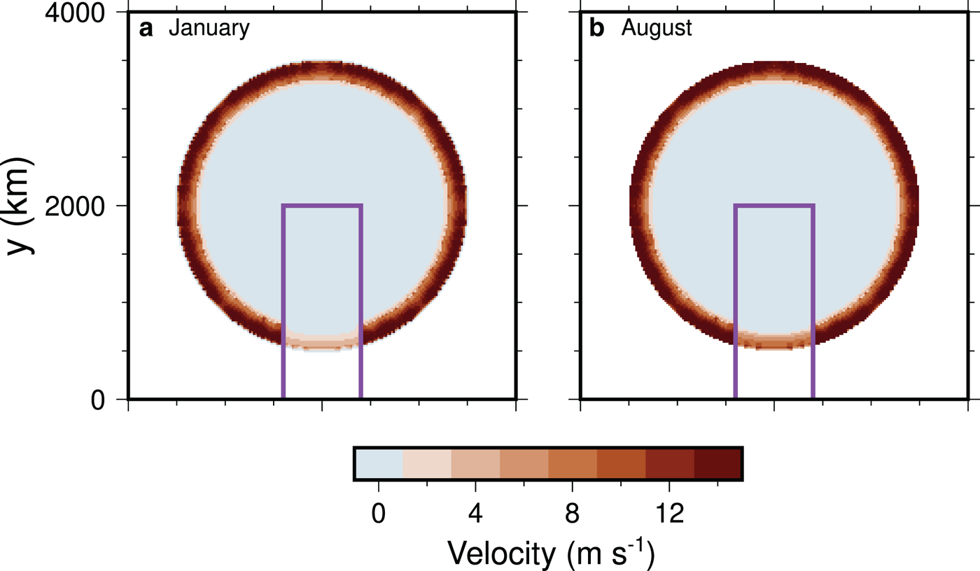
Fig. 5. Comparison of ice sheet surface velocity between the winter and summer for the simulation shown on Figure 3 at 25 000 years. The purple box shows the region that has S f =50% sediment cover. (a) In the winter, the velocity in partially sediment cover is near zero, while the margin regions with continuous cover continue to flow. (b) In the summer, the velocity in partially covered areas increases as a result of the input of water.
3.2.2 Effect of fraction sediment cover
We conducted a series of experiments where we set the strip of reduced sediment cover to be S f = 50%, 80%, 95% and 99% (Figs. S1 and S2). The purpose of this experiment is to see if there is a threshold where sediment deformation becomes important in partially covered regions. In the experiments shown on Figure S1, ϕ sed = 30° for sediment deformation, γ rc = 15° for areas with bare rock, and γ sc = 5° for areas covered in sediment. In the experiments shown on Figure S2, ϕ sed = 20° for sediment deformation, γ rc = 2° for areas with bare rock, and γ sc = 1° for areas covered in sediment. The amount of water reaching the base from the surface is 80%. In the first case sliding is always accomplished through sediment deformation (for instance, Figs. S1 and S2), as the value of γ sc = 5° seems too high to allow for sliding on the ice-bed interface. There is a slight increase in velocity during the summer, as the sediments become replenished and water saturated. In the 50% covered area, the velocity is about half that of the fully covered area, and the difference becomes smaller as a large fraction of area becomes sediment covered. For the second set of experiments, the sliding mechanism in the partially sediment covered areas does switch as water input increases, leading to an increase in velocity. The areas fully covered in sediment never switch to sliding along the base.
3.2.3 Effect of γ rc and γ sc
We tested a variety of values for γ rc and γ sc using S f = 50% sediment cover and ϕ sed of 20 and 30 degrees (Figs. S3 for ϕ sed = 30; 4 for ϕ sed = 20). For areas with 100% sediment cover, a switch from sediment deformation to sliding at the ice-bed interface did not happen unless γ sc < 1°. For areas with incomplete cover, this threshold is γ sc < 2°.
3.2.4 Effect of ϕ sed
We did many of the experiments with ϕ sed = 30° and ϕ sed = 20° (see Figs. S5 and S6) with different values of γ rc and γ sc. With the higher value of ϕ sed, the average velocity is generally slower. During the melt season, the average velocity in the partially sediment covered areas increase more when ϕ sed is lower. When γ rc and γ sc are set to lower values, the lower value of ϕ sed prevents the switch to the base sliding regime likely due to the higher initial velocity. This actually causes the maximum velocity in the ϕ sed = 30° experiments to be higher during the melt season, even though the annual average is lower.
3.2.5 Effect of water input
We tested different values of the fraction of surface meltwater reaching the base, using values of 0%, 5%, 20%, 50%, and 80% (Fig. S7). Using 0% (which would be equivalent to the default in PISM), there is essentially no sliding because there is no water getting into the system, preventing the sediments from filling with water and deforming. When the fraction is ≥20%, the velocity in fully covered areas reaches its standard value for the points we test (i.e. there is enough water entering to saturate the sediments), and the incompletely covered areas start experiencing an increase during the summer. As the fraction of meltwater reaching the base increases, the seasonal increase in velocity also increases.
To test more extreme amounts of water reaching the base, we also artificially changed the climate index to simulate the effects of extreme melting seasons, which is shown on Figure S8. When the index is changed so that the surface temperature is warmer, there is a much greater amount of meltwater being produced. This demonstrates the switching between the cavity and tunnel drainage styles. As mentioned before, this switch limits how low the effective pressure can be, and therefore how fast the velocity is during the summer.
3.3 Glacial cycle simulation
In order to show the effect of different basal conditions on ice sheet evolution, we have repeated the experiment done by Niu and others (Reference Niu, Lohmann, Hinck, Gowan and Krebs-Kanzow2019) for the region covered by the Laurentide and Cordilleran ice sheets in North America. The simulation runs for the past 120 000 years, using an index based on the NGRIP δ 18O record (Andersen, Reference Andersen2004), with the value for full glacial conditions (1) corresponding to the Last Glacial Maximum (LGM) value at 21 000 yr BP, and a value of 0 to represent interglacial conditions at 0 yr BP. The climate forcing is from equilibrium simulations using the PMIP3 protocol from the COSMOS-AWI model (Stepanek and Lohmann, Reference Stepanek and Lohmann2012; Zhang and others, Reference Zhang, Lohmann, Knorr and Xu2013). We have edited the forcing to have zero precipitation outside of the Laurentide-Cordilleran region to prevent ice sheet growth.
We compare the evolution of the ice sheet through the glacial cycle using three simulations. The default simulation (denoted ‘default’) has the default ‘null’ hydrology model used in PISM, where water is only created at the base through geothermal and frictional heating, and basal strength is defined through sediment deformation only (Tulaczyk and others, Reference Tulaczyk, Kamb and Engelhardt2000). The second simulation (denoted ‘basal’) has our new model as described earlier. In the basal simulation, we use γ rc = 2°, γ sc = 1°. The fraction of surface meltwater reaching the base is set to 80% based on Clason and others (Reference Clason2015). Although this may overestimate how much water reaches the base in higher elevation areas, we choose this value in order to test the model. The third simulation, (denoted ‘norock’) is the same as basal, but uses 100% sediment cover over the entire domain. This tests the impact of spatially variable sediment cover on the evolution of the ice sheet.
The sediment properties for North America are derived from the dataset by Gowan and others (Reference Gowan, Niu, Knorr and Lohmann2019) (Fig. 6). In this dataset, there is a parameterization for sediment grain size, and a generalized sediment cover distribution. For the sediment friction angle, we have set ϕ sed = 30° for sand, ϕ sed = 20° for silt, and ϕ sed = 15° for clay. These values are used for all experiments. For sediment cover, the fraction of the surface covered is set to 100% for ‘blanket’ (i.e. complete cover), 80% for ‘veneer’ (i.e. isolated bedrock outcrops), and 50% for ‘rock’ (i.e. widespread bedrock outcrops).
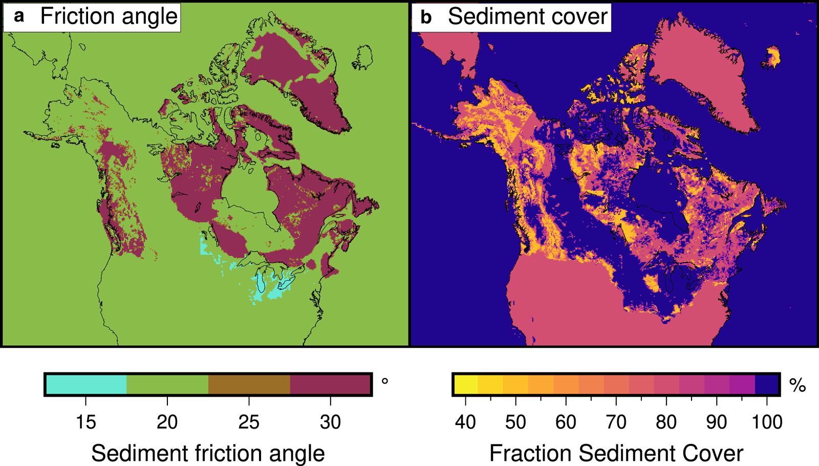
Fig. 6. Sediment properties used in the experiment (Gowan and others, Reference Gowan, Niu, Knorr and Lohmann2019). (a) Sediment friction angle (ϕ sed), used to govern the strength of the sediments. (b) Sediment cover distribution (S f), showing areas of complete and incomplete sediment cover.
A comparison of the default and basal simulations are shown on Figure 7. The results of these simulations show that while the overall volume of default and basal simulations is similar, the distribution of where the ice can be quite different. In the basal simulation, the ice advances faster, which allows more rapid buildup especially in areas with complete sediment cover. This results in places like Hudson Bay becoming fully covered in ice earlier in the simulation (Fig. 8). In the Last Glacial Maximum (20 000 yr BP) time slice, shown on Figure 7, this results in having thicker ice in western Laurentide region than in the default simulation, as the ice is able to flow there easier. The default simulation has thicker ice in the core ice growth centers, which results in an overall greater ice volume. The basal conditions in the basal simulation prevents the buildup of ice, and the volume stays stable through the LGM period. The absolute difference in ice volume between the simulations reaches up to 5 m of sea level equivalent (SLE, i.e. the equivalent water volume of ice divided by the area of the modern ocean).
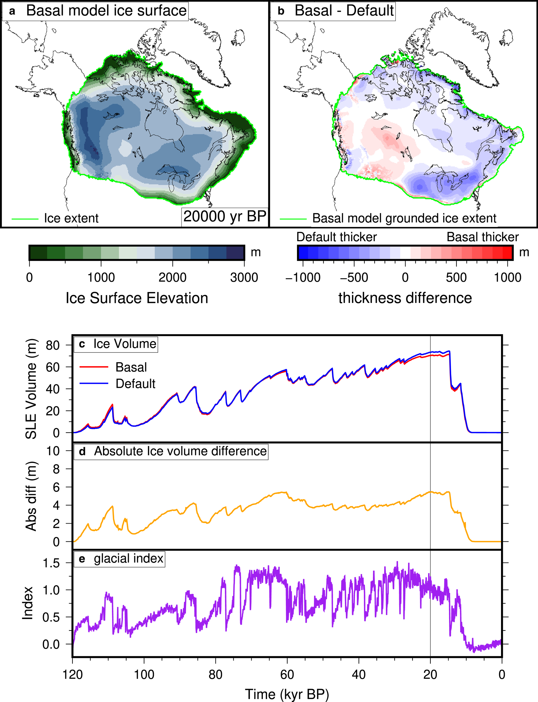
Fig. 7. Results of the glacial cycle simulation, comparing the default and basal simulations. (a) The ice surface elevation of the basal simulation at 20 000 yr BP. (b) The difference between the basal and default grounded ice thickness at 20 000 yr BP. (c) Ice volume evolution of the simulations. (d) Absolute ice volume difference (i.e. the absolute value of panel (b)) between the simulations. (e) Glacial index used in the simulations, based on the Greenland ice core records (Andersen, Reference Andersen2004).
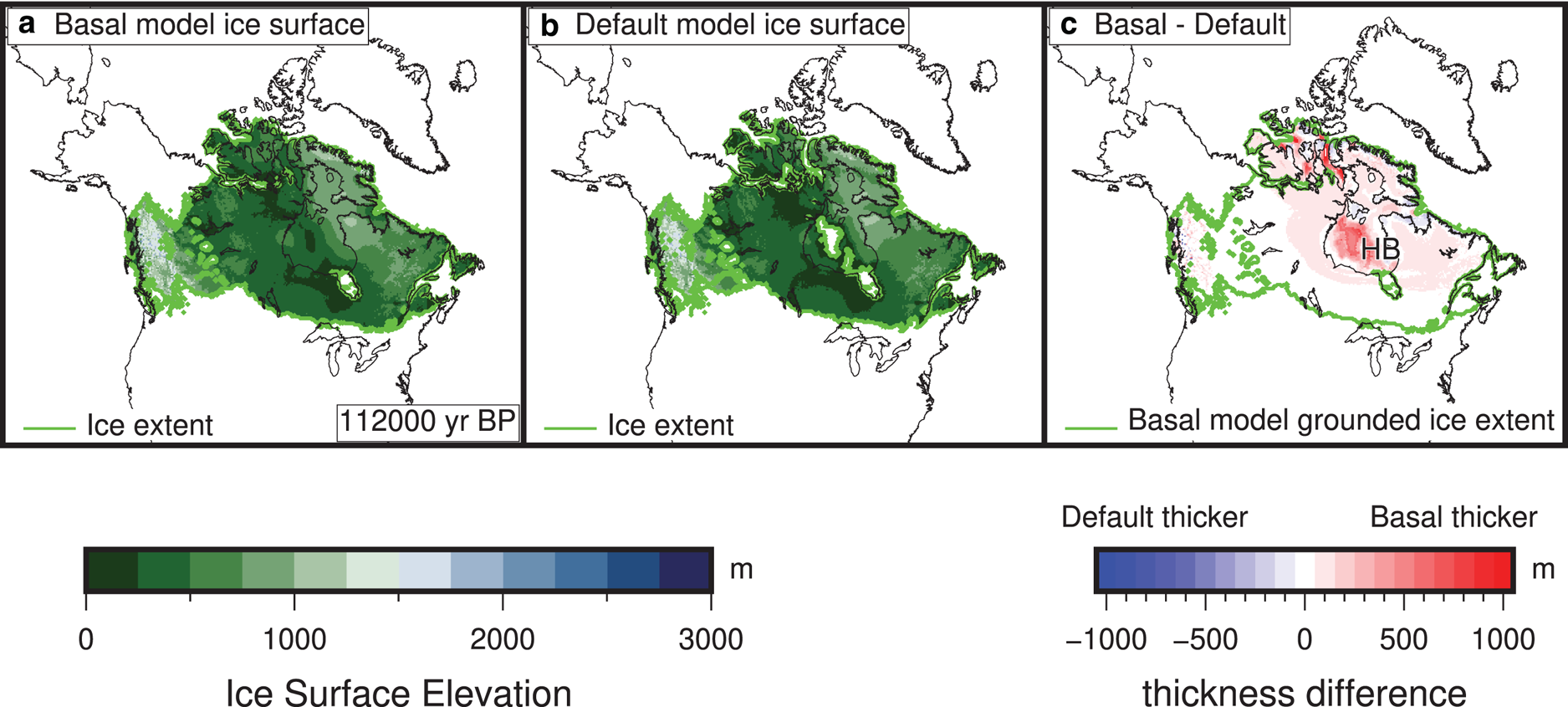
Fig. 8. Early ice advance into Hudson Bay (HB) in the basal simulation. (a) The ice surface elevation of the basal simulation at 112 000 yr BP. (b) The ice surface elevation of the default simulation at 112 000 yr BP. (c) The absolute value of the difference between the basal and default grounded ice thickness. Figures showing the evolution between 116 000 to 111 000 yr BP are shown on Figure S11.
A comparison of the basal and norock simulations are shown on Fig. 9. The simulation with S f =100% cover (Fig. 9) is primarily different in areas that are mountainous, especially in the Cordilleran region (where a significant area has $S_f = 50\percnt$ cover), but also in the mountainous areas on the southeastern part of the ice sheet. This indicates that for the given parameterization, partial sediment cover only has a significant impact on ice sheet evolution where there are also large topographical changes. The lack of sediment cover allows for a more stable ice sheet in mountainous regions. The lower impact of the incomplete covered Canadian Shield on the results shows that a larger value of γ rc or lower value of S f may be needed to provide a contrast in basal conditions between the ‘soft bedded’ and ‘hard bedded’ regions. Alternatively, it may indicate that the contrast in bed conditions is not as significant of a factor in the evolution of the Laurentide Ice Sheet as was previously assumed.
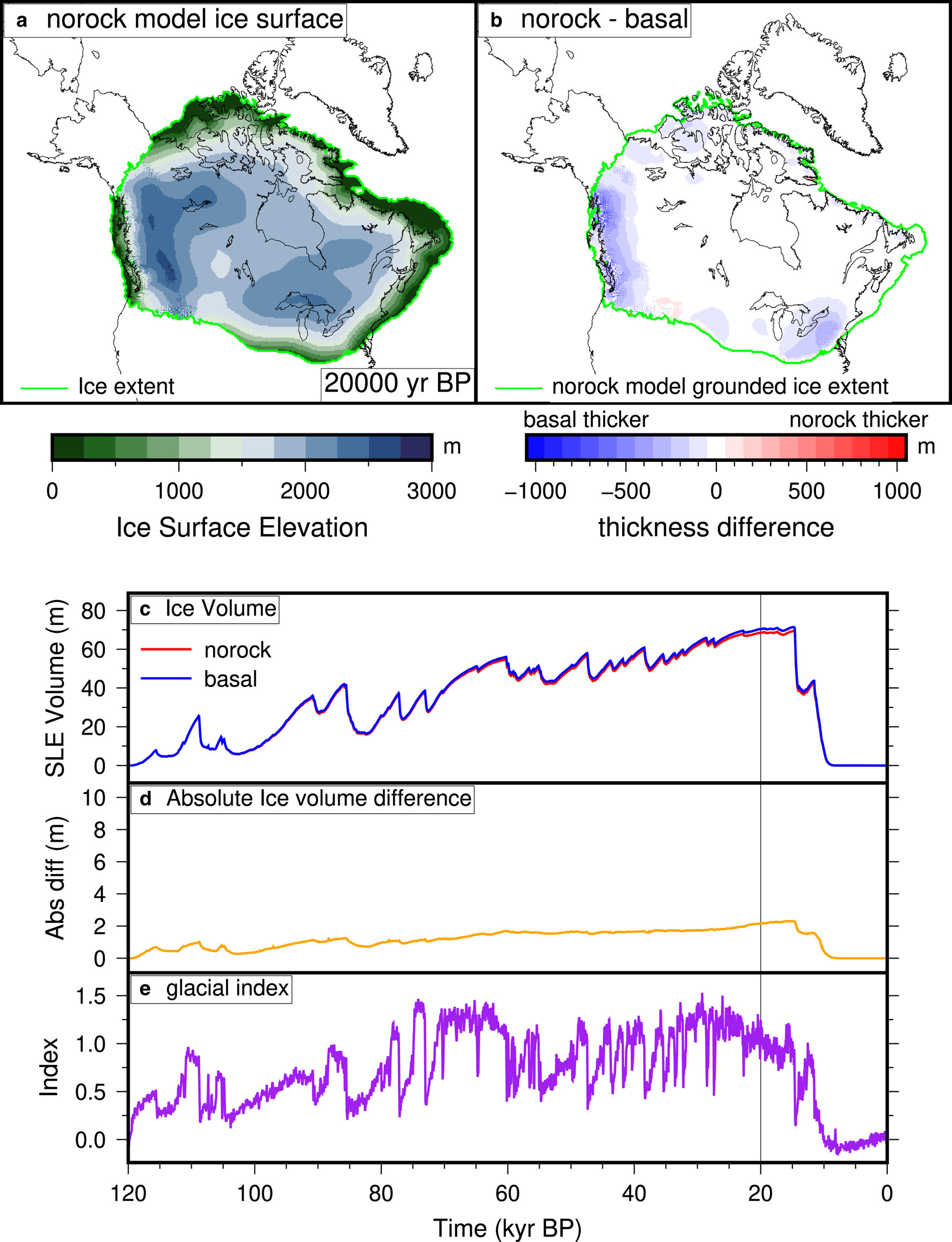
Fig. 9. Same as Figure 7, but comparing a simulation with S f =100% sediment cover (norock) and with spatially variable sediment cover (basal). (a) The ice surface elevation of the norock simulation at 20 000 yr BP. (b) The difference between the basal and norock grounded ice thickness at 20 000 yr BP. (c) Ice volume evolution of the simulations. (d) Absolute ice volume difference (i.e. the absolute value of panel (b)) between the simulations. (e) Glacial index used in the simulations, based on the Greenland ice core records (Andersen, Reference Andersen2004).
A comparison of the velocity between the simulations for the southeastern Laurentide Ice Sheet at 20 000 yr BP is shown on Figure 10. The velocity in the default simulation near the margin of the ice sheet is low throughout the year, which explains why the ice sheet is thicker in this area compared to the basal and norock simulations. The simulations that use the new basal conditions model has a much larger velocity. The basal simulation has patches with lower velocity where there is incomplete cover, which does not happen in the norock simulation. However, these low velocity patches only have a minor impact on the ice thickness (Fig. 9). This may indicate that on longer time scales, the surface mass balance plays a larger role in ice sheet evolution than dynamic ice loss from spatially heterogeneous ice sheet flow in areas without large topography changes, at least in a glacial index style experiment. Alternatively, it may indicate that the coarse spatial resolution we use is unable to promote ice flow into narrow ice streams that would create a more varied topography. There is seasonal variations in velocity of up to 20 m yr−1, which mostly happens along the margin of the ice sheet.
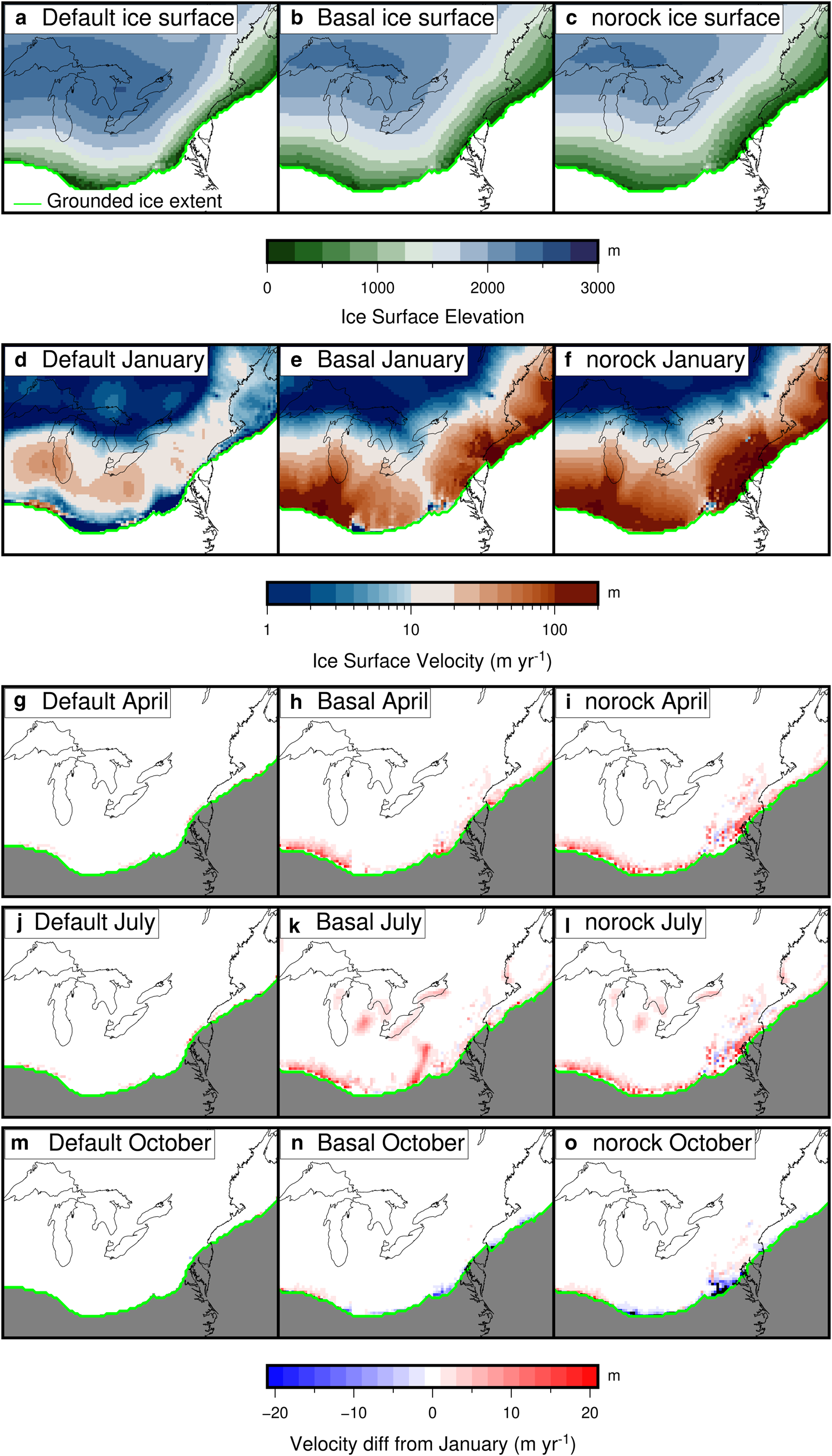
Fig. 10. Comparison of ice surface elevation (a–c) and ice surface velocity in January (d–f) and the difference in velocity compared to January (g-o) for the three simulations for the southwestern Laurentide Ice Sheet at 20 000 yr BP.
The basal conditions model is designed to have low enough complexity to run at glacial cycle timescales. The overhead at fully glacial conditions is roughly double that of the default model. This increase in overhead is largely the result of having seasonally variable water input, which results in generally larger velocity values (Fig. 10). This causes the more computationally intensive shallow shelf stress balance model to be computed over a larger area. The sacrifice in speed is balanced by a more realistic depiction of ice sheet dynamics.
Geologically informed reconstructions of the initial growth of the Laurentide Ice Sheet (e.g Kleman and others, Reference Kleman2010; Gowan, Reference Gowan2021) depict the ice sheet growing from independent domes centered either side of Hudson Bay, eventually merging to form a single ice sheet. This may have happened multiple times during a glacial cycle (Dalton and others, Reference Dalton2019). Our basal conditions model is able to reproduce this behavior easier than the default PISM model (Fig. 8). If repeated ice cover over Hudson Bay happened multiple times, the presence of saturated, deformable sediments recharged by surface meltwater is likely a prerequisite of this behavior. This shows the importance of including seasonal meltwater input to the base, in order to ensure that the sediments under the ice sheet remain saturated. The peripheral regions of the Laurentide Ice Sheet also had low profiles as a result of the weak basal conditions (Mathews, Reference Mathews1974; Beget, Reference Beget1987; Fisher and others, Reference Fisher, Reeh and Langley1985; Wickert and others, Reference Wickert, Mitrovica, Williams and Anderson2013). Our model is better able to create a low profile in peripheral regions than the default model. In places such as the Great Lakes region, the ice thickness is as much as 500 m less than the default model (Fig. 7).
4 Conclusions
We have presented a new basal conditions model for use in the ice sheet model PISM. This model allows us to incorporate spatially variable sediment parameters and basal hydrology that includes meltwater from the surface. Our model runs fast enough to feasibly perform glacial cycle scale simulations. The model, when applied to the Laurentide Ice Sheet, impacts how the ice sheet evolves, and changes the ultimate distribution and thickness of ice. Since the ice sheet is able to dynamically grow at a much faster rate, this provides a more realistic depiction of glacial advance. The primary cause of the changes in dynamic behavior is the addition of meltwater from the surface into the subglacial hydrology system. This allows the sediments at the base to fill with water far easier than in the default model, allowing for sustained sliding. In partially sediment covered areas, there is an increase in velocity during the summer. At glacial time scales, the impact of partially sediment covered areas on the evolution of the ice sheet was not substantial except in mountainous areas. In future studies with a coupled climate forcing, we anticipate that our model will be better able to reproduce geological evidence of ice sheet extent and flow.
Supplementary Material
The supplementary material for this article can be found at https://doi.org/10.1017/jog.2022.125.
Data
The version of PISM 1.0 with our basal conditions model can be found at https://github.com/evangowan/pism_basal. The scripts to generate the idealized circular ice sheet experiments can be found at https://github.com/evangowan/pism_blackboard.
Acknowledgements
This work was funded by the Helmholtz Climate Initiative REKLIM (Regional Climate Change), a joint research project of the Helmholtz Association of German research centers (HGF). This study was also supported by the Bundesministerium für Bildung und Forschung funded project PalMod, and the Program Changing Earth - Sustaining our Future of the Helmholtz Association. Funding also came from an International Postdoctoral Fellowship of Japan Society for the Promotion of Science. Computer simulations were performed on the Cray CS400 (‘Ollie’) supercomputer of AWI. We acknowledge the Ollie administrators, Natalja Rakowsky and Malte Thoma. We acknowledge support by the Open Access Publication Funds of Alfred-Wegener-Institut Helmholtz-Zentrum für Polar- und Meeresforschung. Development of PISM is supported by NSF grants PLR-1644277 and PLR-1914668 and NASA grants NNX17AG65G and 20-CRYO2020-0052. The figures were created with the aid of Generic Mapping Tools (Wessel and others, Reference Wessel2019).
Author Contributions
Evan J. Gowan came up with the concept for the basal conditions model, with input from Caroline Clason and Gerrit Lohmann. Evan J. Gowan wrote the model code with contributions from Sebastian Hinck. Lu Niu and Sebastian Hinck developed the design of the PISM experiments, which were modified by Evan J. Gowan. Evan J. Gowan wrote the manuscript with input from all authors.


 Open access