


Introduction
Lake Vostok is located in central East Antarctica, below a 4 km thick ice sheet. It is the largest subglacial lake on earth with a length of almost 290 km, a maximum width of 90 km, an area of 16 000 km$^2$ (Popov and Chernoglazov, Reference Popov and Chernoglazov2011) and a maximum depth exceeding 1000 m (Popov and others, Reference Popov, Masolov, Lukin and Popkov2012). The ice surface morphology above the lake is characterized by its exceptionally smooth and almost horizontal surface (Fig. 1). This peculiarity, aided by satellite radar altimetry, was instrumental in the lake's discovery (Ridley and others, Reference Ridley, Cudlip and Laxon1993; Kapitsa and others, Reference Kapitsa, Ridley, de Q Robin, Siegert and Zotikov1996). The flat ice surface above the lake has been used to improve surface elevation retrieval methods from radar altimetry (Roemer and others, Reference Roemer, Legrésy, Horwath and Dietrich2007; Schröder and others, Reference Schröder2019) and as target for the determination of ICESat laser campaign biases (Ewert and others, Reference Ewert2012b; Richter and others, Reference Richter2014; Schröder and others, Reference Schröder2017). The satellite laser altimetry dataset provided by ICESat (2003–09; Schutz and others, Reference Schutz, Zwally, Shuman, Hancock and Di Marzio2005) improved the accuracy of surface heights and their spatio-temporal changes in the Lake Vostok area, and was used to observationally demonstrate the hydrostatic equilibrium of the ice-sheet surface over the lake (Ewert and others, Reference Ewert2012b; Schwabe and others, Reference Schwabe, Ewert, Scheinert and Dietrich2014). The laser campaign biases determined over Lake Vostok were applied in the estimation of surface elevation changes and the ice mass balance of the Antarctic and Greenland ice sheets (Ewert and others, Reference Ewert, Groh and Dietrich2012a; Groh and others, Reference Groh2012, Reference Groh2014a, Reference Groh2014b; Shepherd and others, Reference Shepherd2018; Schröder and others, Reference Schröder2019; Shepherd and others, Reference Shepherd2019).
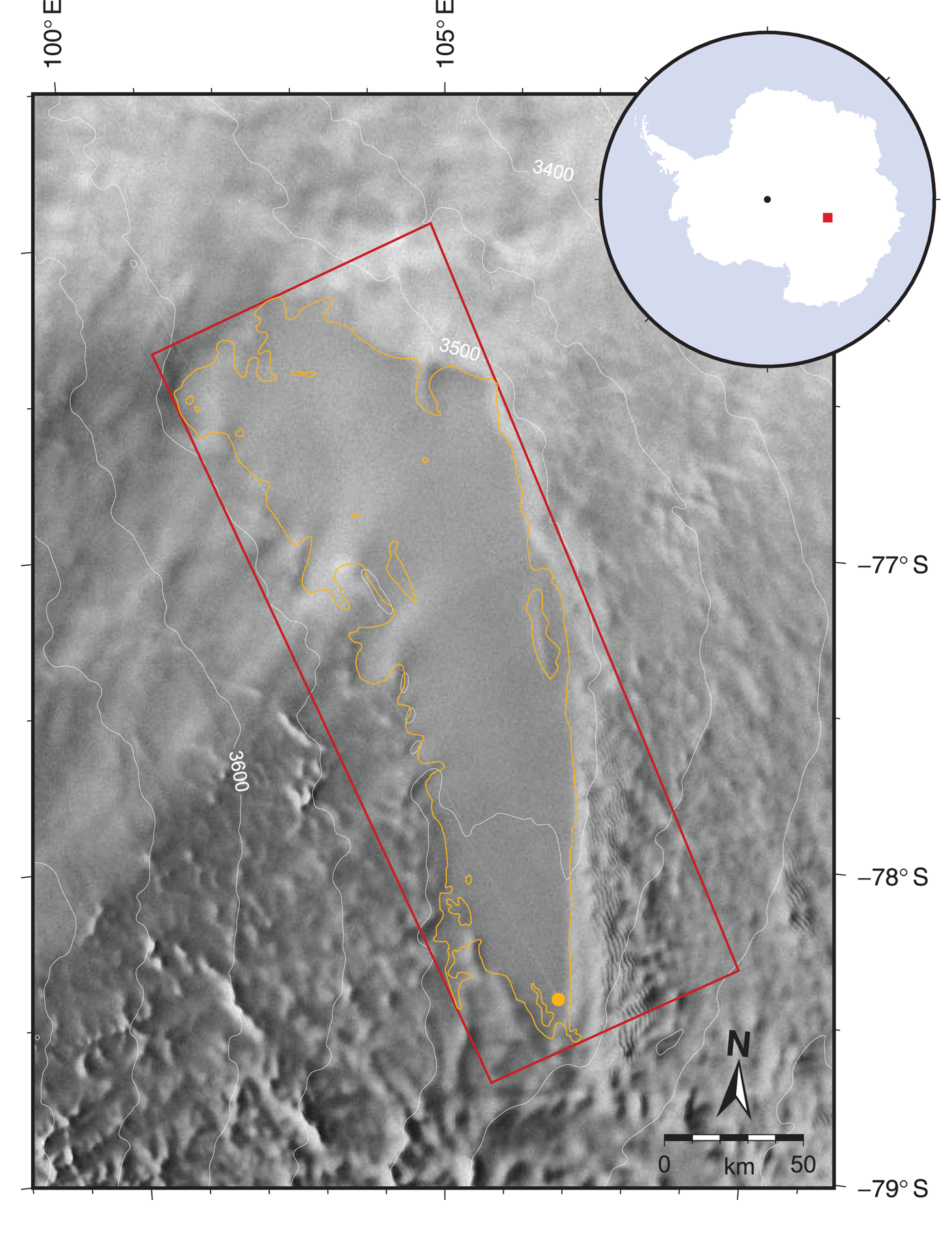
Fig. 1. Map of the area under investigation. Orange: shoreline of Lake Vostok derived from terrestrial radio-echo sounding (Popov and Chernoglazov, Reference Popov and Chernoglazov2011); orange dot: Vostok station; red: model grid domain, corresponds to the map domain of Figs 3, 4–9, 12; white isohypses indicate ellipsoidal surface elevation in metres (Bamber and others, Reference Bamber, Gomez-Dans and Griggs2009); background: RADARSAT amplitude image (Jezek and others, Reference Jezek, Noltimier and Team2001). Inset: location of map area (red square) in central East Antarctica; black dot: South Pole.
Surface accumulation rates are small in this area, ranging from 20 to 35 kg m$^{-2}$ a$^{-1}$
 , and exhibit a regional S–N gradient (Ekaykin and others, Reference Ekaykin, Lipenkov and Shibaev2012; Richter and others, Reference Richter2021). Basal accretion and melting occur simultaneously in different parts of the lake area and maintain a continuous mass exchange between the ice sheet and the lake (Bell and others, Reference Bell2002; Tikku and others, Reference Tikku, Bell, Studinger and Clarke2004). While the bedrock topography allows us to rule out a subglacial water discharge from Lake Vostok (Richter and others, Reference Richter2014), a water inflow through an active hydrological system could produce a water volume increment in the lake (Wingham and others, Reference Wingham, Siegert, Shepherd and Muir2006; Smith and others, Reference Smith, Fricker, Joughin and Tulaczyk2009) potentially detectable as a uniform surface height increase over the lake. The water surface of the lake affects also the ice flow due to the absence of basal friction. Understanding the interplay between height changes, ice flow dynamics and basal ice–water interaction is of particular relevance in the Lake Vostok region for the interpretation of the Vostok ice core and the separation of palaeo-climatic signals from glacio-dynamic effects superimposed in the observable parameters (Petit and others, Reference Petit1999; Salamatin and others, Reference Salamatin, Tsyganova, Popov and Lipenkov2009).
Geodetic fieldwork conducted in the Lake Vostok region since 2001 has contributed to the quantification of firn particle movements and surface height changes over the lake. Static Global Navigation Satellite Systems (GNSS; including the GPS) observations on surface markers during repeated occupations yield velocity components which represent the vertical and horizontal particle movement of a firn particle at the marker base. The vertical particle movement is dominated by a firn-densification driven subsidence (Richter and others, Reference Richter2014). The horizontal velocity components reflect the local ice flow which is, within the lake area, representative for the entire ice column (Wendt and others, Reference Wendt2006; Richter and others, Reference Richter2013). This allows the determination of components of the local ice mass balance (Richter and others, Reference Richter2008, Reference Richter2014). A continuously operating GNSS station at Vostok provides time series of daily 3-D particle positions since early-2008. Lake tides have been shown to produce small vertical particle and surface displacements over Lake Vostok (Wendt and others, Reference Wendt2005). Schröder and others (Reference Schröder2017) derived surface height profiles of high accuracy from kinematic GNSS observations on snow vehicles. Crossovers between kinematic GNSS profiles acquired at different observation epochs allow us to determine local surface height changes. A combination of these complementary observation techniques indicates that ice surface height changes above Lake Vostok have kept within $\pm 2$ mm a$^{-1}$
 over a decade, that the local ice mass balance is very close to equilibrium and that the firn densification occurs almost linearly over several years (Richter and others, Reference Richter2014; Schröder and others, Reference Schröder2017).
However, the observations on which those results rely might be affected by surface or particle height variations over the lake resulting from the hydrostatic response to snow, ice or atmospheric pressure loads. Here, we develop a modelling scheme to derive height changes over Lake Vostok from any given load pattern. This approach is applied to realistic load scenarios to demonstrate the mechanism, spatial patterns and plausible magnitudes of the hydrostatic response. It is further used to predict surface and particle height changes based on input fields of snow-buildup anomalies and atmospheric pressure loads derived from a regional climate model. These predicted height changes are compared to available observational datasets with the aim to (a) explore the observational detectability of load-induced height changes; (b) evaluate the efficiency of our model predictions as corrections to geodetic observables and (c) estimate the impact of the hydrostatic load response on observational results published previously without explicit correction.
Methods
Model setup
We define load as a change in the spatial distribution of mass (due to snow buildup or basal melting/accretion) or pressure at the ice-sheet surface between two points in time (before and after the change). The response to this load is evaluated in terms of the vertical displacement of two particular interfaces: the ice–water interface and the surface of the ice sheet. These interfaces can change their vertical position as a result of two mechanisms: first, a deformation, that is, the vertical displacement of firn/ice particles and, second, the accretion or erosion of firn/ice particles at the interface. In order to discriminate between both contributions in our model we introduce the particle horizon. This concept denotes a laterally continuous set of firn/ice particles within the ice sheet. This horizon participates in the deformation mechanism, through the relative vertical displacement of its constituting particles, but is not affected by the accretion/erosion contribution at the ice-sheet interfaces above and beneath. Illustrative examples for particle horizons are the surfaces of coeval ice particles, manifested as internal layers in radio-echo sounding profiles, whose constitutive particles represented the ice-sheet surface at the time of their accumulation (though a common accumulation time is not a necessary condition for a particle horizon in our case). In the following, we do not consider any (a) water volume change in Lake Vostok (i.e. no influx nor discharge, Richter and others, Reference Richter2014, and imposing a zero net basal mass balance over the lake area); (b) hydrodynamic lake-level variation; (c) change in the vertical firn/ice density profile and (d) vertical solid-earth deformation beneath the subglacial lake (e.g. due to glacial isostatic adjustment or tectonics).
Archimedes’ principle determines the vertical position of the ice-water interface at the base of ice floating in hydrostatic equilibrium on an extended water surface. It relates any load applied to the ice surface with the vertical displacement of the ice-water interface resulting from the hydrostatic adjustment to this load. In the case of Lake Vostok, the extent of the ice body exceeds that of the water surface. The hydrostatic equilibration is then confined to within the area of the subglacial lake. The hydrostatic adjustment to the load causes a bending of the ice sheet, which is assumed unfractured. This implies a finite relative vertical displacement of neighbouring ice columns, limited by the visco-elastic properties of the ice sheet. The lateral smoothness of particle horizon (e.g. ice-water interface) deformation leads to an attenuation of the hydrostatic response towards the lake shore, as well as across abrupt load gradients within the lake area. The hydrostatic ice-water interface adjustment complies, in addition, with the water volume conservation in the lake. This volume conservation leads to ice-water interface displacements also in those parts of the lake area unaffected by the load, but with inverted sign. Hence, load-induced height changes of the ice-water interface are determined by the following three constraints: (a) the hydrostatic equilibrium; (b) the flexural attenuation and (c) the water volume conservation. The surface height change is then obtained by adding the load thickness to the ice-water interface displacement. Figure 2 illustrates the effect of the three constraining processes on the considered interfaces in response to a surface load as, e.g. a snow-buildup anomaly.
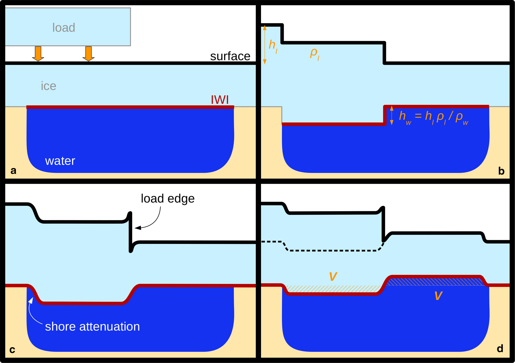
Fig. 2. Schematic cross section of Lake Vostok. (a) Geometry of ice surface (black) and ice-water interface (red) in an initial situation before the application of a surface load. (b) Vertical deformation of the surface and ice-water interface (IWI) due to the hydrostatic equilibration of the load. The load is described by its height $h_{\rm l}$ and density $\rho _{\rm l}$
 ; $h_{\rm w}$
 : vertical ice-water interface displacement; $\rho _{\rm w}$
 : water density. (c) Effect of the flexural attenuation, damping the vertical surface and ice-water interface deformation across the attenuation fringes along the lake shores and the load edge. (d) Effect of the water volume conservation in the lake on the vertical surface and ice-water interface displacements. The water volume $V$
 lost due to the load-induced ice-water interface deformation (hashed area to the left) equals the volume gain (hashed area to the right). The dashed black line shows the equilibrated surface in the case of a pressure load equivalent to the mass distribution of the considered surface load.
A load acting on the surface of the floating ice sheet is described in any place $x$ by the areal load mass density $\kappa ( x)$
 . The areal density of a snow or ice load is determined by the thickness $h_{\rm l}$
 and density $\rho _{\rm l}$
 of the load:

In the case of atmospheric pressure loading the areal density is obtained by dividing the local pressure $P_{\rm l}( x)$ by gravity $g$
 :
:

i.e. the applied pressure can be represented equivalently by adding or subtracting mass atop the ice sheet.
The hydrostatic equilibration of a surface load (prior to accounting for flexural attenuation and water volume conservation) produces a vertical ice-water interface displacement $h_{\rm w}^{( 1) }( x)$ governed by the local areal density $\kappa ( x)$
 , expressed as the equivalent water column height by applying the density of water $\rho _{\rm w}$
 :
:

A positive $h_{\rm w}^{( 1) }( x)$ denotes an upward displacement of the ice-water interface. The hydrostatic response to a spatially non-uniform load produces a vertical deformation of the ice-water interface which follows the opposite of the spatial pattern of the areal density variations over the lake area. The vertical ice-water interface displacement is zero where the ice is grounded, that is, outside the subglacial lake and over islands. We keep the grounding line position fixed, neglecting the small migrations caused by load-induced ice-water interface displacements. The ice-water interface deformation differs from $h_{\rm w}^{( 1) }( x)$
 due to the flexural attenuation at the transition from floating to grounded ice, as well as across steep load gradients. The attenuation is described by a factor $a( x)$
 that depends on the distance to the nearest shore segment and varies from 0 (grounded, no ice-water interface displacement) to 1 (freely floating, complete hydrostatic equilibrium). Hence, the ice-water interface displacement with account for flexural attenuation becomes

For the characteristic attenuation profile we adopt a linear shape over a length $L_{\rm a}$ :
:

where $d( x)$ denotes the distance to the nearest shore segment. The profile length $L_{\rm a}$
 determines the width of the attenuation fringe along the shore, across which the ice-water interface deformation is damped. We adopt a profile length of 10 km. This choice is supported, on the one hand, by the surface deformation observed over Lake Vostok (Wendt and others, Reference Wendt2005) and, on the other hand, by the deviation of the static surface geometry from hydrostatic equilibrium (Ewert and others, Reference Ewert2012b; Schwabe and others, Reference Schwabe, Ewert, Scheinert and Dietrich2014); and will be elaborated on in the Discussion section.
In general, the ice-water interface deformation involves a volume excess $\Delta V$ over the lake area $S$
 :
:

Water volume conservation is ensured through an additional vertical shift of the ice-water interface by $a( x) k$ , where $k$
 is constant over the lake area and $a( x)$
 is, again, the flexural attenuation near the shores. Volume conservation implies that $k = - \Delta V / \tilde {S}$
 , where $\tilde {S} = \iint a( x) {\rm d}S$
 is the effective area on which the volume excess $\Delta V$
 is compensated. Hence, the final expression for the ice-water interface displacement is

Due to the subtraction of $k$ , only the relative differences of the load within lake area are effective rather than the absolute value of the introduced mass or pressure load. In the case of atmospheric pressure loading, the induced surface height change $h_{\rm s}( x)$
 is identical to the vertical ice-water interface displacement $h_{\rm w}( x)$
 . For snow loads, the surface height change is obtained by adding the load height $h_{\rm l}$
 to the ice-water interface displacement:

In general, the spatial patterns and gradients of the ice-water interface and surface deformations depend on the patterns of load distribution and attenuation. Combining Eqns (1), (3) and (8) we see that, in the case of snow-buildup loads and neglecting attenuation effects, the gradients of surface vs ice-water interface displacements relate as $h_{\rm s}/h_{\rm w} = ( h_{\rm l} ( 1-\rho _{\rm l}/\rho _{\rm w}) ) / ( -h_{\rm l} \rho _{\rm l}/\rho _{\rm w}) = 1-\rho _{\rm w}/\rho _{\rm l} < 0$ . The negative sign of this deformation gradient ratio denotes that the hydrostatic equilibration partitions an ice thickening between an upward growth at the surface and a downward growth at the ice-water interface. The surface snow density at Vostok ($\rho _{\rm l} =\, \sim \! 330$
 kg m$^{-3}$
 ) suggests furthermore that surface height change gradients are approximately twice as large as the simultaneous ice-water interface height change gradients.
The calculations are performed on a grid of the lake area (red box in Fig. 1) with 100 m spacing. The attenuation factors within the transition zone along the grounding line and the effective lake area $\tilde {S}$ are the same for any load scenario and are therefore computed only once. The ice-water interface displacement $h_{\rm w}( x)$
 is calculated according to Eqn (7). The maximum gradient within the ice-water interface displacement grid $h_{\rm w}( x)$
 is evaluated. If the gradient exceeds a threshold of 10$^{-5}$
 , the flexural attenuation across load edges is applied. For example, the geometrical description of load patterns can be simplified by polygons delimiting areas of constant areal density (Fig. 2). A polygon segment which separates different surface densities to either side is referred to as load edge. In this case, the load edge attenuation is implemented by smoothing the load areal density grid $\kappa ( x)$
 within a 10 km wide attenuation band centred on the load edge by a linear interpolation between the $\kappa$
 values on either side of the edge (consistent with the linear, 10 km long attenuation profile applied for the shore attenuation). The calculation of the $h_{\rm w}( x)$
 grid according to Eqn (7) is then repeated introducing the smoothed $\tilde {\kappa }( x)$
 grid. The surface height jump at the load edge shown in Figure 2c equals the height of the load in Figure 2a, $h_{\rm l}$
 .
.
Different geometrical load discretizations (patterns) are adopted in the computational experiments presented below: a uniform load within a polygon (pattern P in Table 1), a regional gradient (G) or an areal density field interpolated from the gridcell pattern of a regional climate model onto our computation grid (I).
Table 1. Summary of the diagnostic scenarios for which the hydrostatic response over Lake Vostok is modelled

aLoad patterns denote: P, uniform load bounded by polygon; I, interpolation from RACMO cell centres onto our calculation grid; G, uniform gradient.
Mass changes at the ice base require a special treatment. In this case, the particle horizon to which the flexural attenuation is applied does not coincide with the ice-water interface. Thus, the attenuation and the volume conservation conditions are evaluated over different surfaces (attenuation: particle horizon, e.g. ice surface; volume conservation: ice-water interface). A preliminary particle horizon deformation $h_{\rm p}^{( 1) }$ is determined according to isostasy and shore attenuation:

The ice-water interface displacement implied by this particle horizon deformation and the basal load height $h_{\rm l}$ yields a preliminary volume excess

This volume excess is corrected through an increment to the preliminary particle horizon deformation, analogous to the case of surface loads (Eqn (7)), yielding

The surface height change corresponds to the particle horizon deformation $h_{\rm s}( x) = h_{\rm p}( x)$ and the final ice-water interface displacement is obtained by subtracting the load height

In our calculations we apply a standard water density of $\rho _{\rm w} = 1000$ kg m$^{-3}$
 . For snow loads we adopt the mean density of the uppermost 20 cm snow layer derived from stake and snow pit observations at Vostok station of $\rho _{\rm l} = 330$
 kg m$^{-3}$
 (Ekaykin and others, Reference Ekaykin, Lipenkov, Petit and Masson-Delmotte2003). For basal ice loads we apply an ice density of $\rho _{\rm l} = 923$
 kg m$^{-3}$
 as derived from the Vostok ice core (Lipenkov and others, Reference Lipenkov, Salamatin and Duval1997).
Loading scenarios
We consider snow build-up, basal ice mass changes and air pressure changes as loads. Spatio-temporal snow-buildup variations are represented by the surface mass balance estimates of the regional climate model RACMO2.3p2 (henceforth RACMO; van Wessem and others, Reference van Wessem2018). Stake observations in the Vostok stake farm and along three profiles across the Lake Vostok area were used to validate this surface mass balance model (Richter and others, Reference Richter2021). We use RACMO's surface mass balance estimates on a grid with a spatial resolution of 27 km, over the period 1979–2019 with monthly resolution, to extract snow-buildup load fields over Lake Vostok.
The basal mass balance of the ice sheet floating on top of Lake Vostok is characterized by simultaneous melting and freezing at the ice-water interface in different parts of the lake. Models (Wüest and Carmack, Reference Wüest and Carmack2000; Mayer others, Reference Mayer, Grosfeld and Siegert2003; Thoma and others, Reference Thoma, Grosfeld and Mayer2007; Salamatin and others, Reference Salamatin, Tsyganova, Popov and Lipenkov2009) and the sparse available observations (Bell and others, Reference Bell2002; Tikku and others, Reference Tikku, Bell, Studinger and Clarke2004) agree that basal accretion prevails in the southern half of the lake area, while basal melting dominates in the northern part. Local basal mass balance estimates were derived for ten polygons distributed over the lake area from a combination of 3-D particle displacement velocities observed by GNSS with ice thickness determined by radio-echo sounding (Richter and others, Reference Richter2014). These estimates suggest that the general basal mass balance variation can be approximated by an N–S gradient of 0.2 kg m$^{-2}$ a$^{-1}$
 km$^{-1}$
 .
.
Atmospheric pressure loading is effective over Lake Vostok according to the inverse barometer response to temporal changes in the air pressure field. The air pressure is continuously recorded at Vostok, but the lack of nearby additional meteorological stations impairs the retrieval of air pressure gradients representative for the lake area. According to Wendt and others (Reference Wendt2005) and Richter and others (Reference Richter2014) the N–S air pressure gradient over the lake area varies within $\pm 2$ Pa km$^{-1}$
 . Here, we use the air pressure fields predicted by RACMO over the period 1979–2019 with a temporal resolution of 3 h.
Our modelling scheme is applied to six diagnostic load scenarios. Table 1 summarizes the scenarios, which are briefly described in the following:
Scenario 1 simulates a snow-buildup anomaly of 24.8 mm restricted to the southern part of the subglacial lake. It is intended to visualize the principal concepts of the hydrostatic load response over the subglacial lake through a hypothetical, geometrically simple case, corresponding to Figure 2. The adopted load height represents the maximum snow buildup observed over 1 month (September 1972) within the stake farm record at Vostok station 1970–2019 (Ekaykin and others, Reference Ekaykin2020; Richter and others, Reference Richter2021).
Scenario 2 mimics the annual snow buildup over Lake Vostok according to the mean surface mass balance predicted by RACMO, averaged over the model period 1979–2019.
Scenario 3 examines the effect of the annual basal ice mass change. It applies the adapted calculation procedure in Eqns (9)–(12) and a gradient load pattern, which assumes that the basal mass balance variation over the Lake Vostok area is dominated by an N–S gradient of 0.2 kg m$^{-2}$ a$^{-1}$
 km$^{-1}$
 , implying an ice load height ranging from $-24.4$
 mm (melting, northern shore) to $+ 33.7$
 mm (accretion, southern shore), while conserving the water volume in the lake.
Scenario 4 combines the annual surface (scenario 2) and basal (scenario 3) mass changes. It represents the mean annual load field accounting for both snow buildup and basal accretion/melting.
Scenario 5 represents an extreme monthly snow-buildup load. Among the 488 monthly surface mass balance predictions by RACMO over the period 1979–2019 we chose that month (August 1992) whose surface mass balance field produces the maximum response in terms of the standard deviation (SD) of the ice-water interface displacements $h_{\rm w}( x)$ over the lake.
Scenario 6 exemplifies an extreme event of atmospheric pressure load. The RACMO air pressure time series 1979–2019 were screened to select that air pressure field (22 February 2011 6:00 UTC) which produces the maximum SD of the ice-water interface displacements $h_{\rm w}( x)$ relative to the mean air pressure field over the model period.
Our model does not account for the dynamical ice mass effect of the ice flow. This is especially important for the interpretation of the effects of annual surface mass balance and basal mass balance applied in scenarios 2–4. The observational evidence presented by Richter and others (Reference Richter2014) suggests that the ice sheet in the Lake Vostok region has been very close to steady state over an observation period of 10 years. Under such conditions, the sum of surface mass balance and basal mass balance over the subglacial lake is compensated by the net ice flux into (along the western shore) and out of (eastern shore) the lake area.
Simulation of geodetic observables
We model three types of geodetic observables: (1) surface elevation changes at ICESat ground track crossover locations; (2) particle subsidence rates inferred from repeated GNSS observations and (3) vertical particle displacements derived from continuous GNSS observations at Vostok station. Observables (2) and (3) are physically similar, but differ in their spatial and temporal coverage which affects also the observational accuracy and their sensitivity to different processes. Observable (2) reflects spatially heterogeneous differences between discrete observation epochs, whereas observation set (3) yields local variations over diverse timescales.
(1) We apply our modelling scheme to explore the effect of spatio-temporal variations in snow buildup and air pressure at 60 crossover locations of the ICESat ground track over the lake during the 18 laser operation periods of the altimetry mission 2003–09. The adjustment of surface elevation differences in these crossover locations were used to determine laser campaign biases. Those laser campaign bias determinations assumed a constant surface elevation (Ewert and others, Reference Ewert2012b; Richter and others, Reference Richter2014) or a constant elevation change rate (Schröder and others, Reference Schröder2017) in these calibration locations throughout the mission period. The distribution of these calibration locations is shown in Figure 3. Here, we introduce the surface mass balance and air pressure variations estimated by RACMO into our modelling scheme in order to assess the impact of their neglect in the laser campaign bias estimation. For this purpose, we derive integral estimates for each laser operation period and the entire set of calibration locations, instead of computing individual corrections for all surface elevation observations introduced in the laser campaign bias adjustment. In the case of the snow load this is justified by its relatively long variation timescales. The local response to air pressure variations between the individual altimetric data acquisitions, in turn, is significant but not accounted for in our estimate. Nevertheless, the laser campaign bias are averaged in space ($\approx \!60$
 calibration locations) and time (laser operation periods of $\approx \!1$ month) over multiple satellite passes across the lake area. As will be shown below, these spatio-temporal averages are dominated by the snow load, justifying our determination of integral estimates. Within each laser operation periods, $h_{\rm s}$ are calculated at the 60 calibration locations and with 3 hourly temporal resolution based on the air pressure fields simulated by RACMO. These $h_{\rm s}$ are averaged yielding, for each laser operation periods, the mean surface height change and standard deviation due to the inverse barometer effect. In order to assess the effect of snow-buildup variations, cumulative surface mass balance anomalies (csurface mass balanceA) are derived from the surface mass balance predicted by RACMO, assuming steady state for the RACMO model period 1979–2019. For each laser operation periods a mean snow-buildup field is inferred by weighting the monthly csurface mass balanceA fields proportionally to the number of days of each month contained in the laser operation periods. The $h_{\rm s}$ are computed for all laser operation periods and calibration locations, and are averaged to the mean surface height change, and its SD, due to snow buildup. The combined effect of air pressure and snow-buildup variations on each laser campaign bias results from summing the mean surface height changes derived for both processes, while the SDs are summed quadratically. These estimates can be considered as corrections to the laser campaign biases derived from crossover adjustments over Lake Vostok, improving the bias values by accounting for the loading effects. Henceforth, they are referred to as laser campaign bias corrections. In addition, the computation of the mean surface height changes among the laser operation periods is repeated based purely on the csurface mass balanceA fields, without consideration of the hydrostatic equilibration. This mimics the effect identical surface mass balance conditions would have over grounded ice, thus its comparison with the results that incorporate the hydrostatic adjustment, including the air pressure variations, reveals the impact of the presence of the subglacial lake on the laser campaign bias estimation. Moreover, the effect of the hydrostatic adjustment at individual calibration locations is exemplified by examining the $h_{\rm s}$ variations in four crossover locations. We select two of the 60 calibration locations close to the northern and southern shores, but sufficiently far away from the shoreline for an undamped hydrostatic response ($a( x)$ = 1). Both selected locations are complemented by the closest ICESat crossover locations outside the lake, over grounded ice. The two pairs of locations are shown in Figure 3.


(2) We assess the impact of surface load changes on particle subsidence rates inferred from repeated GNSS observations. Each of the 56 markers reported by Richter and others (Reference Richter2014, Table 1) was occupied during multiple (2–7) Antarctic field seasons between 2001 and 2013 over observation periods between 1 and 60 d. Here, we focus on those 42 markers which are located within the lake area ($a( x) > 0$
; included in Fig. 3). Daily coordinate solutions for each marker and observation day were obtained from the GNSS data processing. Based on these daily solutions vertical velocities were derived which range from $-33$ to $-106$ mm a$^{-1}$ with uncertainties between $\pm 2$ and $\pm 22$ mm a$^{-1}$. The hydrostatic response to surface loads contributes to the vertical particle movement at the base of these GNSS markers and may contaminate the velocity estimates used to describe the long-term particle movement. For each day a coordinate solution is present for any of the considered markers, the hydrostatic response of the ice-water interface to snow-buildup anomalies and air pressure variations is modelled and interpreted in terms of the load-induced particle movement. The monthly csurface mass balanceA grids are interpolated in time to the GNSS observation day, whereas the pressure field for that day is obtained by averaging the 3 hourly model simulations over 24 h. In this way, coordinate corrections are obtained for each marker and observation day. We evaluate the amount by which the application of these corrections changes the reported vertical velocities.(3) The vertical particle movement derived from continuous GNSS observations at Vostok station over 10 years is examined in search of observational evidence for the effects of snow-buildup anomalies and air pressure variations. For this purpose, we use the time series of daily solutions in the vertical coordinate component between early-2008 and late-2018. This represents an update of the time series presented by Richter and others (Reference Richter2014, Fig. 5) and results from a post-processing of dual-frequency GPS observations in differential mode using Bernese GNSS Software (Dach and others, Reference Dach, Lutz, Walser and Fridez2017). Non-linear signals in the vertical particle movement are extracted by detrending the time series. Monthly mean relative vertical particle positions are derived by averaging the detrended daily vertical coordinates within each month. In addition, the ice-water interface displacements our modelling scheme yields at the location of the GNSS station as response to the snow load represented by the monthly csurface mass balanceA fields derived from RACMO are detrended and compared with the observed non-linear position variations. For the detection of the inverse barometer effect on the particle movements observed at Vostok, the time series of daily vertical positions are high-pass filtered (filter width 30 d). The air pressure fields estimated by RACMO with 3 hourly resolution are averaged over 24 h to daily mean pressure load fields. These are introduced into our modelling scheme to yield a time series of the ice-water interface displacement at the GNSS station with daily resolution. This time series is filtered identically to the GNSS position time series.


Fig. 3. Map of the Lake Vostok area (model domain). Grey dots: 60 ICESat track crossover locations for which the impact of the hydrostatic load response is evaluated (Figs 10a, b); blue/red dots and diamonds: two pairs of ICESat crossover locations in the northern (blue) and southern (red) parts of the lake used to compare the surface height change between hydrostatically balanced (dots) and grounded (diamonds) ice (Fig. 10c); green triangles: location of 42 GNSS surface markers (Richter and others, Reference Richter2014) for which the impact of the hydrostatic load response on vertical particle velocities is evaluated.
Results
Loading scenarios
Our modelling results for the six diagnostic scenarios are summarized in the Figs 4–9. Maps of the load distribution (top), the surface height change (centre) and the ice-water interface displacement (bottom) are shown for each scenario. They are summarized in the following. Some statistics are given in Table 2.

Fig. 4. Scenario 1: hypothetical uniform snow-buildup load of 24.8 mm over the southern part of Lake Vostok. (a) Load distribution. (b) Induced surface height change. (c) Induced ice-water interface displacement.
Table 2. Modelled vertical displacements (mm) over Lake Vostok in response to the scenarios listed in Table 1
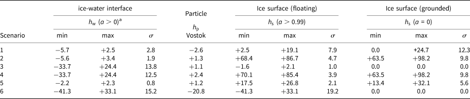
a $h_{\rm w}$ , vertical displacement of the ice-water interface; $h_{\rm p}$
 , vertical displacement of a firn particle at Vostok station; $h_{\rm s}$
 , surface height change; $\sigma$
 , SD of the spatial variation over the considered gridcells.
Scenario 1: snow-buildup anomaly of 24.8 m over the southern part of Lake Vostok
Despite the fact that the load applies only for the southern part of the lake area both the ice surface (Fig. 4b) and the ice-water interface (Fig. 4c) are displaced all over the lake area. The ice-water interface subsides by $-5.7$ mm within the southern, loaded part and rises by $+ 2.5$
 mm in the northern part. The ratio between subsidence and rise is determined by the ratio between the loaded and free area within the lake. The ice surface rises all over the lake area. In the southern part it rises by $+ 19.1$
 mm, which is less than the snow buildup. Over the northern part of the lake, not exerted to the snow load, the surface rise equals the ice-water interface rise. Over the grounded ice outside the lake the north-south step in the load height is sustained in the surface height change. Within the lake area, in contrast, this step is damped. The shape of the transition across the load edge is determined by our assumptions on the attenuation profile. Genuine snow loads usually do not involve a discontinuity as implied by our polygon abstraction. The constant levels of surface height change in both the northern and southern parts are superimposed by the imprints of islands due to the flexural attenuation of the ice-water interface deformation.
Scenario 2: annual snow buildup over Lake Vostok
The imposed load pattern (Fig. 5a) is characterized by a SSE–NNW gradient within the range of $+ 63.5$ to $+ 98.2$
 mm over our model domain. This gradient and range is preserved in the surface height changes over grounded ice (e.g. to the east and west of the lake; Fig. 5b). Within the lake area, the gradient is damped in result of the ice-water interface deformation, which has a gradient opposite to that of the load: it subsides in the northern part (up to $-5.6$
 mm) and rises in the southern part (up to $+ 3.4$
 mm; Fig. 5c). The magnitude of the ice-water interface deformation is only about one-tenth of the magnitude of the load height because only the relative differences over the lake area are effective upon the ice-water interface due to the water volume conservation condition. The patterns of ice-water interface deformation and surface height change are superimposed by the attenuation at shores and islands.

Fig. 5. Scenario 2: mean annual snow-buildup load according to the RACMO regional climate model. (a) Load distribution. (b) Induced surface height change. (c) Induced ice-water interface displacement.
Scenario 3: annual basal ice mass change over Lake Vostok
Both the load and the induced surface height changes of this scenario are spatially restricted to within the lake area (Fig. 6). The basal mass balance gradient is hydrostatically balanced by the surface height change, multiplied by a factor $( \rho _{\rm w} - \rho _{\rm l}) / \rho _{\rm w} = 0.077$ , and modulated by the attenuation towards the shores. Over the hydrostatically balanced portion of the lake area ($a( x) > 0.99$
 ), the surface height change ranges from $-1.6$
 mm (northern lake part) to $+ 2.1$
 mm (south). The ice-water interface displacement resembles the load height gradient with opposite sign and reaches extrema at $-33.7$
 mm and $+ 24.4$
 mm close to the southern and northern termini of the lake, respectively.

Fig. 6. Scenario 3: spatial variation in annual basal mass balance approximated by a uniform N–S gradient of 0.2 kg m$^{-2}$ a$^{-1}$
 km$^{-1}$
 over Lake Vostok. (a) Load distribution. (b) Induced surface height change. (c) Induced ice-water interface displacement.
Scenario 4: annual surface mass balance plus basal mass balance
Outside the lake the surface height change (Fig. 7a) is identical to the adopted snow-buildup load (and to that in scenario 2, Fig. 5b). Over the lake, the S–N surface rise gradient is significantly reduced. The ice-water interface displacement (Fig. 7b) is clearly dominated by the basal mass balance gradient, with subsidence in the south (up to $-33.7$ mm) and a rise in the north (up to $+ 24.4$
 mm), opposite to the ice-water interface deformation expected from the snow buildup alone (Fig. 5c). Figure 7c depicts the vertical deformation of a particle horizon within the ice sheet. It shows a smooth pattern, compliant with the attenuation towards the shore. The north-south gradient of the displacement of the ice column (from $-6.9$
 mm in the north to $+ 5.3$
 mm in the south) is opposite to the gradient of ice-water interface displacement.

Fig. 7. Scenario 4: combined response to annual snow buildup (Fig. 5a, derived from RACMO) and basal mass balance (Fig. 6a, approximated as regional gradient). (a) Induced surface height change. (b) Induced ice-water interface displacement. (c) Induced vertical displacement of a particle horizon within the ice sheet.
Scenario 5: extreme monthly snow buildup
The snow load for August 1992 (Fig. 8a) is characterized by an S–N gradient within a range of $+ 13.4$ to $+ 32.1$
 mm over our model domain and amounts to about a quarter of the mean annual snow buildup. The resulting surface height change (Fig. 8b) is damped over the lake area. In the hydrostatically balanced portion it is within $+ 17.5$
 to $+ 26.8$
 mm. The ice-water interface responds essentially by a tilt with a rise (up to $+ 2.3$
 mm) in the south and subsidence (up to $-2.2$
 mm) in the north, modulated by the shore attenuation (Fig. 8c). While screening over the 488 monthly surface mass balance fields in search of the extreme event, we calculated, for every month, the SD of the spatial variability of the surface height change $h_{\rm s}$
 over the hydrostatically balanced part of the lake area (i.e. over all gridcells with $a> 0.99$
 ). The average of the 488 SDs is 0.6 mm. In contrast, for the snow load itself, the average SD calculated in the same way is 0.9 mm.

Fig. 8. Scenario 5: extreme monthly snow-buildup load (August 1992) according to RACMO predictions 1979–2019. (a) Load distribution. (b) Induced surface height change. (c) Induced ice-water interface displacement.
Scenario 6: extreme event of air pressure change
The atmospheric pressure load anomaly of 22 February 2011 6:00 UTC (Fig. 9a) represents a low-pressure event with an intensity increasing from south to north by 8.4 hPa. The ice-water interface displacement and the surface height change are identical (Fig. 9b). They correspond to a gradient, modulated by the shore attenuation, with a subsidence of up to $-41.3$ mm in the south and a rise of $+ 33.1$
 mm at the northern boundary of the hydrostatically equilibrated lake area.

Fig. 9. Scenario 6: extreme atmospheric pressure load according to RACMO predictions. (a) Load distribution: air pressure difference between 22 February 2011 at 6:00 UTC and the mean pressure field 1979–2019. (b) Induced surface height change, identical to the ice-water interface displacement.
Simulated observables
The combined effect of snow-buildup anomalies and atmospheric pressure loads on the surface height averaged over each laser operation periods and the 60 ICESat calibration locations in the Lake Vostok area is shown in Figure 10a (red). The formal uncertainties included in Figure 10a are derived from the SDs of both load responses in the calibration locations (1$\sigma$ ). Over the mission period 2003–09, these laser campaign bias corrections were within a range of 26 mm, whereas their formal confidence intervals vary between $\pm 2$
 and $\pm 5$
 mm. The SD of these laser campaign bias corrections amounts to 7 mm, compared to a 34 mm SD of the uncorrected laser campaign biases (Schröder and others, Reference Schröder2017). The comparison of these laser campaign bias corrections with those calculated hypothetically without consideration of the hydrostatic equilibration (black with grey confidence interval) suggests that the presence of the subglacial lake has a negligible impact on the temporal surface height variability that affects the laser campaign bias and their uncertainties.

Fig. 10. Impact of hydrostatically balanced surface loads on ICESat laser campaign biases derived for crossover adjustments over Lake Vostok. (a) Red: corrections (dots) and their formal uncertainty (vertical bars, 1$\sigma$ ) of laser campaign biases for snow-buildup anomalies and atmospheric pressure load changes derived from the RACMO regional climate model including the hydrostatic response. Black: corrections and uncertainty (grey band) of laser campaign biases in the case of a hypothetical absence of the subglacial lake; top axis annotation: laser operation periods. (b) Individual contributions of the snow-buildup anomalies including the hydrostatic response (green) and air pressure variations (blue) to the laser campaign bias corrections and their uncertainty. (c) Comparison of the effect of snow-buildup variations on hydrostatically balanced (solid lines) and grounded (dashed) crossover locations in the northern (blue) and southern (red) parts of the lake (Fig. 3), between the laser operation periods; tiny dots: response to air pressure changes in the hydrostatically balanced calibration locations in the northern (blue) and southern (orange) lake parts during the laser operation periods at 3 hourly resolution.
The individual contributions from the snow load and air pressure variations to the laser campaign bias corrections are split up in Figure 10b. The laser campaign bias corrections derived as temporal averages over each laser operation periods are clearly dominated by the snow-buildup anomalies (green). The response to air pressure variations is insignificant when averaged over the time of an laser operation periods (blue). Thus, in our estimation the inverse barometer affects only the uncertainty, rather than the value, of each laser campaign bias correction. At the same time, the hydrostatic adjustment of the ice surface to the snow load manifests itself primarily in a reduction of the uncertainty of the laser campaign bias corrections (i.e. spatial variability within each laser operation periods), without significantly affecting their values. This explains the similarity of the laser campaign bias corrections with and without account of the hydrostatic equilibration with respect not only to their values but also their uncertainties (Fig. 10a): the reduction in the uncertainty due to the hydrostatic adjustment of the snow load is largely compensated by the uncertainty contribution of the inverse barometer response.
Figure 10c compares the impact of the snow load on individual crossover locations over grounded (dashed lines) and hydrostatically balanced portions of the ice sheet (solid lines) in the southern (red) and northern (blue) parts of the lake area. The general coherence between the four curves, but also with respect to the average over all 60 calibration locations (Fig. 10b, green), indicates that the surface height changes at individual locations are dominated by large-scale snow-buildup variations. The spatial correlation between the southern locations (red), or between the northern pair of locations (blue), is higher than the correlation between hydrostatically balanced or grounded sites. During almost all laser operation periods the spread between the hydrostatically balanced locations (solid lines, correspond to circles in Fig. 3) is narrower than between locations on grounded ice (dashed lines, diamonds in Fig. 3). This illustrates the compensating effect of the hydrostatic equilibration on the snow-load induced surface height changes. In the background of Figure 10c, tiny dots depict the response of the surface height to air pressure changes in the southern (orange) and northern (blue) hydrostatically balanced calibration locations within each laser operation periods with 3 hourly resolution. It suggests that, despite practically vanishing mean values when averaged over an laser operation periods, over shorter timescales the inverse barometer effect in individual locations may vary within 5 cm. A closer inspection reveals (e.g. for laser operation periods 2B and 3H) that this large range results from antipodal deviations in the southern and northern locations, consistent with a seesaw response over the lake.
The laser campaign biases determined by Schröder and others (Reference Schröder2017) imply an apparent trend of $+ 11.7\pm 3.4$ mm a$^{-1}$
 . Our laser campaign bias corrections show a linear trend of $+ 2.1$
 mm a$^{-1}$
 , thus their application would reduce slightly the apparent laser campaign bias trend within the stated confidence interval.
The ice-water interface displacements our modelling scheme yields for the 42 GNSS markers in response to snow-buildup anomalies and air pressure loads are applicable as corrections to the daily GNSS solutions in the vertical coordinate component. The mean absolute magnitude of these daily corrections, averaged over all markers and occupations, amounts to 4 mm, with extreme values of $-23$ and $+ 10$
 mm. These corrections are dominated by the contribution from the response to air pressure changes with values in the range between $-35$
 and $+ 14$
 mm and with a mean absolute magnitude of 11 mm. The contribution from the response to the snow load ranges from $-12$
 to $+ 19$
 mm, with a mean absolute magnitude of 8 mm. The contributions of the inverse barometer and snow-buildup anomalies to the daily coordinate corrections are of opposite sign for the majority of observation days and GNSS sites, compensating each other to a large extend.
These coordinate corrections have only a minor impact on the vertical velocities. The mean absolute magnitude of the velocity change, averaged over the 42 markers, amounts to 0.5 mm a$^{-1}$ (i.e. 0.7%). The velocity changes implied by the corrections range from $-0.4$
 to $+ 3.0$
 mm a$^{-1}$
 . They depend on (a) the time span between first and last observation, because the impact of a single correction or observation decreases with an increasing observation time span; (b) the duration of each occupation, because the dominant response to air pressure forcing reduces significantly with increasing integration time and (c) the location of the GNSS site within the lake, because the shore distance determines the magnitude of the load-induced particle displacements through the shore attenuation.
Our daily particle displacement corrections have only a minor impact on the residual RMS deviation of the daily coordinate solutions after subtracting the linear velocity model. On average, the application of the corrections changes the residual RMS by 0.7 mm in terms of mean absolute magnitude, i.e. $\sim$ 10% of the RMS of the observations. The corrections do not produce a decrease in residual RMS in the majority of the time series. This suggests that the observation residuals are dominated by other effects, such as uncertainties in the reference frame stability in the GNSS positioning, rather than load-induced particle movements.
Figure 11a shows the continuous record of daily coordinate solutions in the vertical component derived from GNSS observations at Vostok station 2008–18. This time series, interpreted in terms of the vertical motion of a firn particle at the base of the GNSS marker, is characterized by a steady subsidence due to firn densification, very well approximated by the linear trend (black line superimposed over the daily solutions represented by orange dots). The residual deviations from this linear model remain within the range of $-15$ to $+ 26$
 mm throughout the 10 years observation period (Fig. 11b), while 68% of the daily residuals fall within the observational uncertainty of $\pm 5$
 mm (Richter and others, Reference Richter2014). Monthly mean residuals are derived from this time series (black curve in Fig. 11b). In Figure 11c, these 119 monthly mean residuals are compared with the vertical particle displacements our modelling scheme predicts in response to snow-load variations according to the RACMO model. This scatter plot demonstrates a much broader variation of the observed non-linear particle displacements compared to the predicted snow-load-induced displacements. This is also reflected by the SD of the observations of 4.4 mm compared to 0.8 mm of the model predictions. The Pearson correlation coefficient amounts to 0.19.

Fig. 11. Vertical particle displacements $\Delta H_{{\rm GNSS}}$ derived from continuous GNSS observations at Vostok station and comparison with the modelled response to snow-buildup anomalies and air pressure loads. (a) Variation in daily vertical coordinate solutions with respect to the ITRF2014 reference frame (orange dots), interpreted as vertical position of a firn particle at the marker base; black line: linear model (velocity). (b) Residual vertical coordinate variations after subtraction of the linear model (orange dots); black: monthly mean residual particle height change; grey: modelled particle response to air pressure loads according to RACMO at daily resolution. (c) Scatter plot of monthly mean residual particle height changes derived from GNSS observations with the modelled particle response $h_{\rm p}$
 (surface mass balance) to snow-buildup anomalies derived from surface mass balance predictions of the RACMO regional climate model. (d) Scatter plot of high-pass filtered particle height changes derived from GNSS observations with the modelled particle response $h_{\rm p}$
 (inverse barometer) to air pressure loads according to RACMO at daily resolution; black line: linear Deming regression model between both time series.
The high-pass filtered variations of the observed daily residuals are compared in Figure 11d to the predictions of the particle response at the GNSS site to air pressure changes according to RACMO. This scatter plot reveals no such disparity in the variability between observations and the model; the SD of the observed variations amounts to 2.5 mm, slightly smaller than that of the predicted inverse barometer response of 3.1 mm. The correlation coefficient of 0.44 indicates a moderate correlation between both time series, which is statistically significant at a 99% confidence level. The Deming regression slope is estimated at 0.80.
Discussion
The results for our diagnostic scenarios demonstrate that even localized loads exert a response of the ice-water interface and surface all over the lake. Loads of uniform areal density, on the other hand, produce no ice-water interface and particle height change, and the induced surface height change is then identical to the load height as in the case of grounded ice. In general, the displacement gradient of the ice-sheet interface to which the load is applied (i.e. surface or ice-water interface) is dominated by the accretion/erosion mechanism, that is, the load height gradient which, in turn, exceeds the gradient of hydrostatic particle horizon deformation by a factor that depends on the density ratio between lake water and the load. For this reason, the gradients of modelled surface displacements are always greater than (surface mass load) or equal to (pressure load) those of the ice-water interface displacement, except for the case of basal load changes. The surface response to snow loads is, consequently, dominated by the load height (scenarios 2 and 5). The hydrostatic equilibration tends to level off the spatial variation in snow-load-induced surface height changes, reducing the spatial SD from 0.6 to 0.9 mm over the hydrostatically balanced portion ($a( x) > 0.99$ ). On the other hand, the response to air pressure variations is effective only over the lake and adds spatio-temporal surface height variability. Over short periods (up to several days; e.g. individual elevation profiles derived from satellite altimetry or kinematic profiling, short GNSS marker occupations), the total surface response is dominated by the response to spatio-temporal air pressure variations which may reach $\pm 4$
 cm in favourable locations and events (Fig. 9b). However, the local response to the air pressure decreases rapidly with integration time due to the stationarity of the forcing. Therefore, over periods of a month or longer (e.g. ICESat laser operation periods), the effect of hydrostatically balanced snow-buildup anomalies exceeds that of the inverse barometer (Fig. 10). Richter and others (Reference Richter2014) estimate magnitudes of a few centimetres for the surface deformations over Lake Vostok induced by both snow-buildup anomalies and atmospheric pressure loading, and our modelling results confirm this.
The accuracy of the model predictions depends on the correctness of the assumptions made in our modelling and the quality of the input forcing, in our case the air pressure and surface mass balance fields provided by RACMO. A likely imperfection of our model setup is the assumption of the rather simple attenuation profile, including the adopted attenuation profile length, which may result in inaccurate attenuation factors and response magnitudes at individual sites. Our choice of a 10 km profile length is based on observed surface deformations (Wendt and others, Reference Wendt2005) and the surface geometry over Lake Vostok (Ewert and others, Reference Ewert2012b; Schwabe and others, Reference Schwabe, Ewert, Scheinert and Dietrich2014). It corresponds to the upper bound of the range given by Vaughan (Reference Vaughan1995) for ice shelves and is consistent with the generalized proportionality to the ice thickness by a coefficient between 2 and 3 (Wendt, Reference Wendt2005). Wendt and others (Reference Wendt2005) use surface deformation profiles derived from SAR interferograms to infer a damping factor $\beta$ and elastic modulus for the ice sheet in the Lake Vostok area according to the model of 2-D elastic bending for a grounding line of constant curvature and constant ice thickness (Rabus and Lang, Reference Rabus and Lang2002). The value obtained for $\beta$
 of 0.122 km$^{-1}$
 corresponds to a decay length $\beta ^{-1}$
 of 8.2 km. Ewert and others (Reference Ewert2012b) and Schwabe and others (Reference Schwabe, Ewert, Scheinert and Dietrich2014) combine a regional DEM derived from satellite altimetry, an ice thickness model derived from terrestrial and airborne radio-echo sounding and a geoid model merging airborne and satellite gravimetry to quantify the deviation of observed ice surface elevations over Lake Vostok from hydrostatic equilibrium. The results indicate that the violation of hydrostatic equilibrium is confined to within shore attenuation fringes of 10 km width. Nevertheless, it could be argued that the width of the elastic attenuation of the dynamic equilibration of load changes exceeds that of the static attenuation because the latter might include an additional plastic deformation component; and that the uncertainty in the forcing field of the deformations analysed by Wendt and others (Reference Wendt2005) does not allow a strong constraint on the derived decay length. Figure 12 illustrates the impact of the choice of the attenuation profile length on the modelled hydrostatic response by comparing the ice-water interface deformation patterns due to an identical surface load (Fig. 12a, corresponding to scenario 1) assuming attenuation profile lengths of 10 km (Fig. 12b) and 20 km (Fig. 12c). It becomes evident that the broader attenuation implied by longer profile lengths flattens the ice-water interface deformation and approximates the observable surface height changes towards the case of grounded ice.

Fig. 12. Effect of the choice of the attenuation profile length on the modelled hydrostatic response to surface loads. (a) Load areal density, corresponding to diagnostic scenario 1 (Fig. 4). The areal density is expressed as negative equivalent water height, which corresponds to a hydrostatic ice-water interface displacement without account of flexural attenuation and water volume conservation. (b) Vertical ice-water interface displacement in response to the load depicted in panel (a) adopting an attenuation profile length $L_{\rm a} = 10$ km. (c) Vertical ice-water interface displacement in response to the load depicted in panel (a) adopting an attenuation profile length $L_{\rm a} = 20$
 km.
km.
RACMO's predictions of spatio-temporal surface mass balance variations in the Lake Vostok area, introduced as snow loads in our modelling, have demonstrated a very good agreement with in situ observations when averaged over 1 year or longer periods (Richter and others, Reference Richter2021). However, that comparison suggests also a considerable uncertainty in the surface mass balance variations estimated by RACMO over sub-annual timescales affected, for example, by a poor representation of the seasonal surface mass balance cycle and a subestimation of the range of monthly surface mass balance variations at Vostok. Thus, the disparity in the variability between monthly observations and the modelled load response (Fig. 11c) may result, in part, from uncertainties in snow-buildup simulations for individual months. Similar limitations can be expected also for the air pressure forcing fields derived from RACMO. We conclude that RACMO is able to provide reliable estimates on typical magnitudes of surface loads, allowing insights into the principal features of the hydrostatic load response demonstrated in our scenarios. But the uncertainties inherent to the estimates of the RACMO version used here regarding the spatio-temporal variations in surface mass balance and air pressure at maximum resolutions (spatial: 27 km; temporal: surface mass balance – monthly, air pressure – daily) do not yet allow to reproduce load-induced particle and surface height changes consistent with the sparsely available observations. This suggests that a determination and application of reliable corrections of geodetic observables for hydrostatic load responses depend on further improvements in the accuracy and resolution of the forcing fields. For this reason, we limit our assessment of loading effects on the ICESat laser campaign bias determination to integral estimates (Fig. 10) rather than to re-adjust the laser campaign biases applying individual corrections.
Nevertheless, our results constrain the magnitude of load-induced effects in GNSS-derived subsidence rates, ICESat laser campaign biases and the implied apparent trend. The monthly mean observed non-linear coordinate variations at our continuous GNSS station at Vostok (Figs 11b, c) are not explained by the modelled response to the snow load, but are dominated by other causes. One alternative process potentially responsible for residual particle displacements could be the non-linearity of the subsidence produced by the firn densification underneath the GNSS marker. In fact, a gradual slowdown in the densification-induced subsidence is expected when the marker base reaches depths of increased firn densities and lower densification rates. However, this effect is probably effective on timescales longer than the range of periods that compose the observed residual coordinate variations ($\sim$ 3–15 months; Fig. 11b). The elastic response of the solid earth to tidal and non-tidal atmospheric and ocean loading is corrected in the GNSS data processing, and possible residual effects are not expected to reach amplitudes comparable to those of the observed non-linear height changes. A possible cause for such cyclic variations can be sought in artificial coordinate fluctuations introduced by instabilities in the terrestrial reference frame used to fix the geodetic datum in the GNSS data processing. This observation calls for the high-pass filtering of the coordinate time series for the detection of an inverse barometer response (Fig. 11d). The load–response corrections derived for the velocities determined by the repeated GNSS observations on our markers are similar in magnitude to the effect of lake tides (Richter and others, Reference Richter2014). They confirm the uncertainty estimates those authors attributed to the reported velocities and validate the conclusions drawn from their interpretation.
What conclusions do our results allow regarding the suitability of Lake Vostok for the ICESat laser campaign bias determination? ICESat acquires individual surface elevation profiles over Lake Vostok within very short periods (s). Therefore, the elevations along such a profile can be affected by an inverse barometer response similar or even larger in magnitude than the 3 hourly predictions illustrated in Figure 10c (tiny dots in the background). The maximum effects can be expected at the extremes of the hydrostatically balanced area along a profile roughly aligned with the lake axis but, due to the seesaw behaviour, these local deviations largely cancel out in the adjustment of profiles sampled by multiple, well-distributed crossover locations. The impact of the hydrostatic load responses on laser campaign biases determined by crossover adjustments over Lake Vostok is dominated by the snow-load height. Figure 10a demonstrates that a practically identical temporal variability would affect an laser campaign bias determination under similar conditions over grounded ice (e.g. Hofton and others, Reference Hofton, Luthcke and Blair2013; Gunter and others, Reference Gunter2014). However, the choice of Lake Vostok as calibration target benefits from additional advantages, apart from the very low temporal surface height variability compared to other parts of the Antarctic Ice Sheet. One advantageous peculiarity is the smooth, almost specular surface geometry of the ice sheet over the subglacial lake (Fig. 1), which minimizes interpolation errors and slope-dependent effects. But also the climatical conditions characterized by predominantly high air pressure, low humidity, relatively low wind speeds, rare occurrences of cloud cover and surface snowdrift, as well as the optical conditions implied by the high elevation, favour the availability and quality of laser altimeter data.
In order to be observationally detectable, snow-buildup anomalies must be sufficiently intense to stand out against measurement noise and other processes affecting surface height observations. Along-track gradients in the surface elevation profiles provided by ICESat are indicative of spatial anomalies in the snow buildup accumulated between the laser operation periods. In the case of a repeat-track analysis focused on the temporal deformation of the elevation profile, the detectability of snow-buildup anomalies is determined by the precision of consecutive elevations along the profile, which is estimated at $\pm 2.5$ cm over Lake Vostok (Richter and others, Reference Richter2014). This SD corresponds to the surface height change ranges our scenarios (1, 2, 4 and 5) predict within our model domain. Thus, the snow accumulated during 1 month in an extreme case (scenarios 1 and 5) produces at Lake Vostok a surface height change just at the detectability threshold. In general, anomalies and gradients of the snow accumulated between the laser operation periods would be more easily detected over the grounded ice surrounding the lake because (a) the surface height change gradients are damped above the subglacial lake due to the hydrostatic equilibration and (b) the along-track surface deformation observed over the lake has to be corrected for the response to air-pressure changes between the profile acquisition times. On the other hand, ICESat's along-track precision decreases over grounded ice as the surface roughness and slopes increase.
Reprocessed CRYOSAT-2 and ENVISAT satellite radar altimetry data presented by Schröder and others (Reference Schröder2019) might achieve almost a similar elevation precision over the flat ice surface above Lake Vostok. One drawback of the conventional (low resolution mode in the case of CRYOSAT-2) radar altimetry is the coarse spatial resolution with which load-induced surface height change patterns can be inferred. In addition, temporal surface height changes derived from radar altimetry can be affected by changes in the signal penetration between the data acquisition times. Surface elevation profiles derived from kinematic GNSS profiling on snow mobiles could also provide evidence for snow-buildup anomalies. Schröder and others (Reference Schröder2017) estimate a typical surface height precision between 2 and 3 cm for most of their profiles. However, the peculiar conditions in the Lake Vostok region make intensive GNSS profiling a logistic challenge, and a dedicated observation of loading effects would require a priori knowledge of their manifestation in space and time to optimize the track configuration.
Continuous GNSS observations above the subglacial lake may support the determination of snow-buildup anomalies through monitoring local, non-linear particle height variations of daily resolution with an accuracy of $\pm 5$ mm. These time series have the potential to contribute to the separation of the responses to snow loads and air pressure changes between the acquisition times of altimetry data or kinematic GNSS profiles, making use of the different temporal signature of both loading processes. However, the available record at Vostok station is affected by the flexural attenuation close to the southern tip of the lake with an attenuation factor only weakly constrained at present. A GNSS site located close to the southern and northern limits of the area of complete hydrostatical equilibration ($a( x) = 1$
 ) would provide a better sensitivity to surface loads. Also a continuous air pressure recording in the northern part of the lake would help to constrain the contribution of the inverse barometer to N–S gradients in surface and particle height changes. Yet, a continuous operation of either a GNSS station or meteorologic sensors outside the permanently occupied Vostok station remains a challenge.
Conclusions
We model the response of the ice sheet above Lake Vostok to three loading processes – spatio-temporal changes in snow buildup, air pressure and basal melting/accretion – by combining the hydrostatic balance, the flexural attenuation of ice-sheet deformation and water volume conservation. Our results show that expectable height changes of the ice surface and particle horizons are close to the detectability thresholds of geodetic observation techniques. They lead to three principal conclusions: first, observational evidence of the loading processes and the response mechanism is at present subject to an unfavourable signal-to-noise ratio over most of the time and space sampled by available datasets. Exceptional load magnitudes would be required for a successful correlation between geodetic observations and the model response derived from a quantitative description of the forcing load. Second, the accuracy with which simultaneous processes (e.g. firn densification, water volume changes) are retrievable from geodetic observables can be improved by applying corrections for load-induced height changes. These corrections can be determined by our model but suffer, at present, from uncertainties in our modelling of flexural attenuation and from uncertainties in forcing fields derived from regional climate models. However, the impressive progress those models achieved recently in predicting the surface mass balance with annual resolution gives faith that soon they will provide accurate input for our model also at monthly resolution. Third, the narrow quantitative constraints our results put on the impact of the considered load processes corroborate the conclusions previous studies drew from observations without explicit correction for load-induced effects, including ICESat laser campaign biases derived from crossover adjustments over Lake Vostok (Schröder and others, Reference Schröder2017), statements on the local ice mass balance (Richter and others, Reference Richter2008, Reference Richter2014) and the systematic impact of the firn densification on stake accumulation observations (Ekaykin and others, Reference Ekaykin2020).
ICESat-2 allows a great step forward in the observation of surface height changes over Lake Vostok (Markus and others, Reference Markus2017). The improvements this new mission offers over its predecessor in terms of spatial coverage, temporal resolution and elevation accuracy are vital for the monitoring of load-induced surface deformation. Our model provides the link between observed deformation patterns and the load fields. Especially, across the subglacial lake shores observed surface deformation profiles will not only help to validate or correct the attenuation profile adopted in our modelling, but also provide new insights into the mechanical properties of the ice sheet in the remote interior of East Antarctica.
Acknowledgements
surface mass balance and air pressure predictions of the RACMO2.3p2 model were provided to the authors by Jan Melchior van Wessem. All figures and part of the computations were produced using the Generic Mapping Tools (Wessel and others, Reference Wessel2019). This study was jointly funded by the German Research Foundation (DFG, grants SCHE1426/20-1, HO4232/4-2, DI473/20-1, DI473/34-1 and DI473/38-1) and the Russian Foundation for Basic Research (RFBR, grants 17-55-12003-NNIO and 10-05-91330-NNIO-a).


 Open access