


Introduction
The rapid drainage of glacier-impounded lakes is not uncommon for most mountainous and polar regions of the world. Today, dangerous outbursts of water bodies in the Caucasus, Altai, Tien Shan, Pamir, Himalayas, Alps, Patagonian Andes, Alaska and other mountainous regions are well known (Post and Mayo, Reference Post and Mayo1971; Haeberli, Reference Haeberli1983; Haeberli and others, Reference Haeberli, Kääb, Mühll and Teysseire2001; Huggel and others, Reference Huggel, Kääb, Haeberli, Teysseire and Paul2002; Bajracharya and Mool, Reference Bajracharya and Mool2009; Wilcox and others, Reference Wilcox, Wade and Evans2014; Zaginaev and others, Reference Zaginaev2016; Petrov and others, Reference Petrov2017; Chernomorets and others, Reference Chernomorets, Petrakov, Aleynikov, Bekkiev and Viskhadzhieva2018; Emmer, Reference Emmer2018; Wilson and others, Reference Wilson2018; Bhambri and others, Reference Bhambri2019). Antarctic oases are coastal regions free from ice sheets with areas of several tens to several thousand square kilometres. They are typified by distinct microclimates, the existence of seasonal streams, non-freezing lakes, cryogenic soils and biota (Cook, Reference Cook1900; Kotliakov and Smolyarova, Reference Kotliakov and Smolyarova1990). Another notable feature of such oases is the sudden drainage of lakes. The instability of the glacier-impounded and englacial lakes in Antarctic oases has been known since the construction of the first Antarctic stations and field bases (Vaigachev, Reference Vaigachev1965; Kaup, Reference Kaup1998). Mostly, outburst floods do not damage infrastructure and, hence, remain unnoticed. However, some of them have drastic consequences. For instance, in the summer of 1960, one of the lakes in the eastern part of the Schirmacher Oasis (Queen Maud Land in East Antarctica) experienced a sharp 3.5 m rise in water level. This led to the drainage of the lake through a collapsed snow dam. The streamflow had a discharge of 7 m3 s−1, and flowed to the Novolazarevskaya Station, which was under construction. The expedition staff immediately dug a channel to drainage the water and save the station from flooding (Averyanov, Reference Averyanov1965). Another example concerns lakes Razlivnoye and Glubokoe located in the area of the Russian field base Molodezhnaya (Enderby Land, East Antarctica). The depletion of these water bodies is cyclical. Outbursts occurred in 1962, 1966, 1969, 1988, 1997, 2006 and always had consequences for infrastructures (Kaup, Reference Kaup1998). The last drainage occurred in 2018 and lasted 5 days from the morning of 19 January to the evening of 23 January. The powerful flow demolished several metal structures of the overpass (Boronina and others, Reference Boronina, Chetverova, Popov and Pryakhina2019). Outburst floods also occur due to the drainage of lakes in the Bunger Hills, Wohlthat Mountains, Fisher Massif but descriptions are mainly presented in technical reports or Russian scientific journals (Klokov and Verkulich, Reference Klokov and Verkulich1994; Melnik and Laiba, Reference Melnik and Laiba1994; Dvornikov and Evdokimov, Reference Dvornikov and Evdokimov2017).
Nevertheless, one of the most powerful and unusual catastrophic floods occurred on 30 January 2017 in the Larsemann Hills (Princess Elizabeth Land, East Antarctica). This drainage involved Boulder Lake, Lake Ledyanoe and an englacial reservoir located in the eastern part of the Larsemann Hills next to the Russian field bases Progress-1 and Progress-3 (Fig. 1). The englacial reservoir does not have an official name, but we marked as Lake Dålk. The outburst flood take place as follows. Boulder Lake is supraglacial in origin and practically always covered with ice. In the summer of 2017, due to intense snow melting, a thin supraglacial layer of water was formed on its ice surface. We believe that drainage of the supraglacial layer of water provoked an overfill of the Lake Ledyanoe with its subsequent overflow into the Lake Dålk. Because of the water inflow, Lake Dålk increased in volume until a critical pressure threshold caused it to drainage through an englacial channel. This caused collapse of the overlying ice resulting in a 183 m × 220 m depression (Fig. 2). Outburst drainage lasted 2.5–3 days. The hazardous hydrological phenomenon did not result in human casualties, but the depression destroyed the route connecting the Russian Progress Station and the Chinese Zhongshan Station with the airfield. Logistics activities of the Russian Antarctic Expedition (RAE) were temporarily disrupted (Popov and others, Reference Popov, Pryakhin, Bliakharskii, Pryakhina and Tyurin2017b). There was no information about the catastrophic drainage of the Boulder, Ledyanoe and Dålk lakes until 2017. There was also no direct evidence for the existence of the englacial water body in the area of the Progress-1. Today, Larsemann Hills is one of the most important logistics centres not only for the Russian expedition but also for the Chinese, Indian and Australian Antarctic expeditions. There is an intensively operated aerodrome, which is used for complex airborne geophysical surveys by the Russians and Chinese. Therefore, the investigation of active lakes in this region is extremely important and relevant.
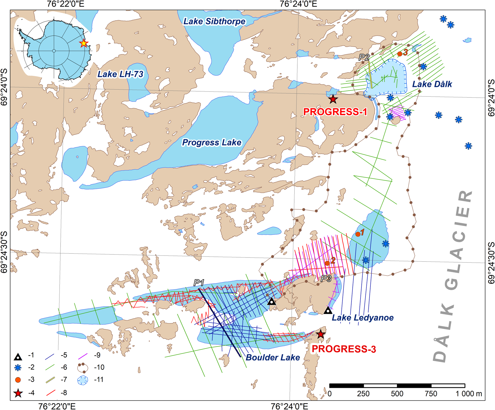
Fig. 1. Variety of field studies of the 63rd and 64th RAE (2017–19) in the area of the Boulder, Ledyanoe and Dålk lakes. (1) Water gauges; (2) glaciological stakes; (3) core drilling; (4) field bases; GPR soundings at frequencies: (5) 75 MHz; (6) 150 MHz; (7) 200 MHz; (8) 500 MHz; (9) 900 MHz (GPR profiles P1 – see in Fig. 3; P2 – see in Fig. 6; P3 – see in Fig. 8); (10) tachometric survey; (11) depression. Background by ADD (Reference ADD2016).
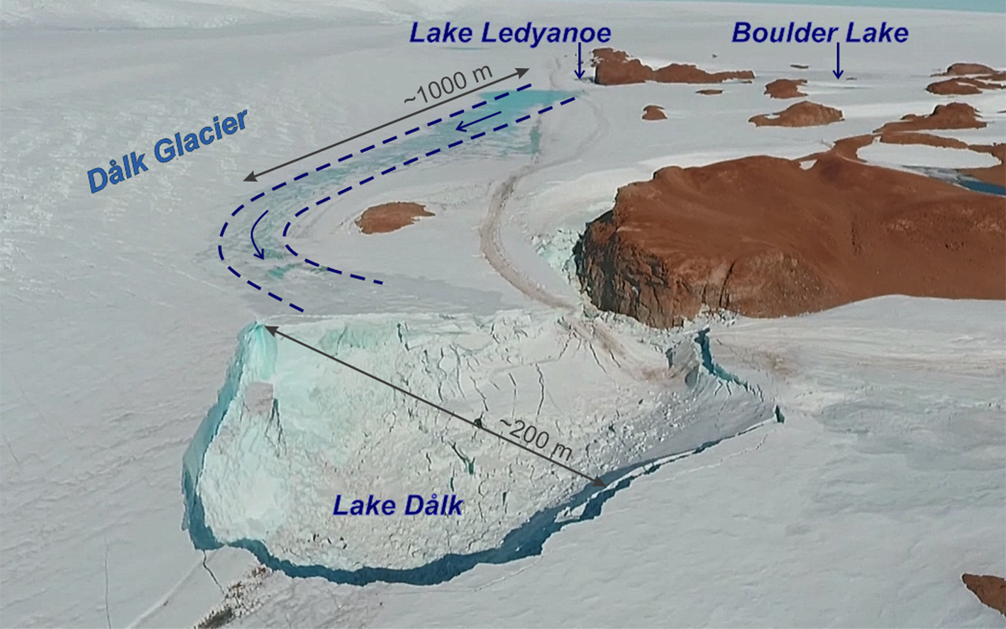
Fig. 2. Photo of the depression on Dålk Glacier. Photo by A.V. Mirakin, January 2017.

Fig. 3. GPR time-section through Boulder Lake and the supraglacial layer of water. (1) Direct wave; (2) reflection from the water-table of Boulder Lake (interface between ice and water); (3) fold reflections from the water-table of Boulder Lake; (4) near-surface crevasses; (5) reflection from the bottom of Boulder Lake; (6) shoreline of Boulder Lake, (7) reflection from the ice–water interface, which is the bottom of the supraglacial layer of water. For the location of the GPR profile, see Fig. 1.
Researchers have encountered sharp subsidence of the ice surface in other areas, similar to that formed in Dålk Glacier. A number of Antarctic studies described cases of ice surface subsidence due to subglacial lake outbursts (Wingham and others, Reference Wingham, Siegert, Shepherd and Muir2006; Fricker and others, Reference Fricker, Scambos, Bindschadler and Padman2007, Reference Fricker, Carter, Bell and Scambos2014; Fricker and Scambos, Reference Fricker and Scambos2009; Smith and others, Reference Smith, Fricker, Joughin and Tulaczyk2009). Evatt and Fowler (Reference Evatt and Fowler2007) have done mathematical modelling of this process. However, the mechanism described in that publication is different from ours, since lakes Boulder, Ledyanoe and Dålk are not subglacial.
This study summarises and clarifies the current state of knowledge on the flood that has occurred in the Broknes Peninsula in 2017. We investigate reasons for the outburst of the system of lakes Boulder, Ledyanoe and Dålk. We present a phenomenological model of depression formation in the place where Lake Dålk was located. In addition, we carry out mathematical modelling of the outburst of each of the three lakes and estimate the hydrographs, channel diameters, volume and duration of floods.
Study region
The hydrological system of three outburst lakes Boulder, Ledyanoe and Dålk is located on the Broknes Peninsula, which is part of the Larsemann Hills in East Antarctica. Dålk Glacier is situated southeast of the peninsula (Fig. 1). A young structural-denudation topography and an undeveloped hydrological network led to the formation of a large number of lakes of various genesis in this area (Gillieson and others, Reference Gillieson, Burgess, Spate and Cochrane1990). Broadly they can be classified as supraglacial ponds, englacial lakes, epiglacial lakes (which are located on the boundary between the rocks and the continental ice sheet) and proglacial lakes that occupy local topography depressions and sometimes are dammed by snowfield (Hodgson, Reference Hodgson2012; Govil and others, Reference Govil, Mazumder, Asthana, Tiwari and Mishra2016). Many of the water bodies are shallow (depth ~5 m), but some of them are relatively deep (up to 50 m) including the system of Boulder, Ledyanoe and Dålk lakes (Fig. 1). In our study, we focus on three types of lakes, namely supraglacial, epiglacial and englacial.
Boulder Lake is a supraglacial type and is located near the Russian field base Progress-3. The lake is usually frozen, but during the Austral summer, lasting from December to January, its parts adjacent to the rocks may be free from ice. Meltwater from the glacier and snow on the rocks is the main source of accumulation of this water body. Little research has been done to explore Boulder Lake that makes it one of the least studied lakes in the Broknes Peninsula. The investigations of the lake are complicated because of the thick ice cover (up to 18.5 m), which demands the use of ground-penetrating radar (GPR) soundings. However, the geophysical research of the lakes on the Broknes Peninsula has begun only since 2017. In warm seasons, the supraglacial layer of meltwater forms on the ice surface of Boulder Lake.
The genesis of Lake Ledyanoe is typical for Antarctic oases. This water body is located on the boundary between the rocks and the continental ice sheet. The formation of this type of lake (epiglacial) determines the surface albedo, which is a key control of surface melt in Antarctica (Lenaerts and others, Reference Lenaerts2017). A low albedo of the rocks increases air temperatures and facilitates melting by increasing the absorption of solar energy (Kingslake and others, Reference Kingslake, Ely, Das and Bell2017). As a result, melt ponds are formed adjacent to low-albedo areas such as an exposed rock that protrudes through the ice sheet. The bowl of Lake Ledyanoe is partly rocky and partly icy. Melting of the glacier ice is the main source of water inflow to the water body. Sometimes the ice dam is partially destroyed or thawed during the summer seasons, leading to lake drainage (Popov and others, Reference Popov, Pryakhin, Bliakharskii, Pryakhina and Tyurin2017b; Boronina and others, Reference Boronina, Chetverova, Popov and Pryakhina2019).
Lake Dålk is the third lake in the hydrological system. This lake was located inside Dålk Glacier, next to the Russian field base Progress-1. There were no visible signs of the existence of Lake Dålk until 2017, however, on 30 January 2017, a large depression appeared in the former lake's location. We suggest that the depression was formed due to the catastrophic englacial drainage of Lake Dålk (Popov and others, Reference Popov, Pryakhin, Bliakharskii, Pryakhina and Tyurin2017b; Boronina and others, Reference Boronina, Popov and Pryakhina2018). Our understanding of the sequence of events is described in detail in the following sections.
The depression on Dålk Glacier was 183 m × 220 m in size and had an area of 31 900 ± 100 m2. Its bottom consisted of blocks of ice that had fallen during the collapse of the ice roof. There were crevasses around the depression suggesting the presence of stresses in Dålk Glacier. In 2018, the depression was slightly covered with snow, but its shape remained almost unchanged.
Methods
In this section, we discuss the methods that allow us to compile the phenomenological model of the occurred outburst, and estimate the drainage of the lakes. For this reason, the section contains methodological features of field research, calculation algorithm of flowlines and a brief description of the mathematical model.
Field studies
The study of drainage basins and lakes of the Broknes Peninsula was carried out during two field seasons in 2017–19 (the 63rd and 64th Russian Antarctic Expeditions). The variety of investigations is depicted in Fig. 1. In general, we monitored the water level in Boulder and Ledyanoe lakes, performed depth surveys using GPR soundings and a depth gauge, and studied the englacial network between Boulder Lake, Lake Ledyanoe, and the depression using GPR soundings. In addition, we did core drilling to study the structure of the upper part of the glacier in the area. Moreover, we surveyed the heights of the glacier surface in the area between the Progress-3 field base and the depression and obtained its precise dimensions and configuration. The current velocity of Dålk Glacier was tracked using eleven fixed glaciological stakes attached to GNSS geodetic satellite equipment. In this section, each type of research will be described in detail.
GPR soundings. Three types of GPR systems were used for the fieldwork. It was the GSSI SIR-3000 (Geophysical Survey Systems, Inc., USA) with antennas at the frequency of 200 and 900 MHz, the Zond12e GPR (Radar System, Inc., Latvia) with antennas at the frequency of 75 and 500 MHz and the OKO-2 (Logis Ltd., Russia) with antennas at the frequency of 150 MHz. The GSSI and Zond12e radar systems have 12-bit analogue-digital converter (ADC), while the OKO-2 has 9-bit ADC that provides a vertical resolution of a few centimetres or better. GSSI GPR research at 200 MHz was used for reconnaissance studies in the area of Progress-1 field base in the 2012/13 field season (58th RAE). We have collected one GPR profile with a length of ~152 m over the englacial Lake Dålk. The year after the outburst flood (2017/18) GPR soundings by the GSSI SIR-3000 at the frequency of 900 MHz and the OKO-2 at the frequency of 150 MHz were used to survey the area between Boulder Lake and the depression which formed in the place of Lake Dålk. The goal was to study the englacial structure of Dålk Glacier in the area where water flow was observed during the 2017 outburst flood. Data were collected along the profiles (Fig. 1). The distance between the profiles was ~20–50 m. The total length of the profiles in this area was ~13 km. We also used the GSSI SIR-3000 at the frequency of 900 MHz to study the depths and ice thickness of Lake Ledyanoe. The total length of the profiles was 490 m. The Zond12e GPR radar system at frequencies of 75 and 500 MHz and the OKO-2 at the frequency of 150 MHz have been used mostly to identify the exact position of the shoreline of the lakes Boulder and Ledyanoe and to determine the depths and ice thickness of Boulder Lake during the field seasons of 2017/18 and 2018/19. Survey profiles are depicted in Fig. 1. The frequency of soundings was selected based on the estimated depth of the lake. Initially, soundings at 150 MHz were performed that were followed by 500 MHz soundings for the shallow water areas and 75 MHz for other deep-water parts of the lake. The total length of GPR profiles on Boulder Lake and its surrounding area was 26.2 km. The GPR surveys were supplemented with measurements of lake depths in wells, using a depth gauge to improve the accuracy of the results. As such, 95 wells on Boulder Lake and 32 ones on Lake Ledyanoe were drilled to measure the water column depth and the thickness of the ice above the water. The measurements of water column depth were done to within ~10 cm, i.e. ~0.5–1%. Measurements of ice thickness of the lakes have been done with an accuracy of 1 cm.
Processing of GPR data was carried out in Radan 7 (Geophysical Survey Systems, Inc., USA), Prism 2.60 (Radar System, Inc., Latvia) and also Geoscan32 (Logis Ltd., Russia) software. We used horizontal filtering with different windows from 20 to 50 traces, depending on the quality of the collected GPR data, to reduce the correlated noise. The accuracy of GPR research on the depth is defined by the velocity of the electromagnetic wave propagation in the media. This velocity was estimated in two ways. The first one is based on modelling the travel-time curves of the diffracted waves from point reflectors. This was estimated based on 280 reflections from the crevasses in ice (Sukhanova and others, Reference Sukhanova, Popov, Boronina, Grigorieva and Kashkevich2020) in the framework of the multilayer model (Popov, Reference Popov2017a). The resulting high variance of permittivity due to the different structures of the glacier, is also confirmed by the ice core drilling. According to Sukhanova and others (Reference Sukhanova, Popov, Boronina, Grigorieva and Kashkevich2020), an average permittivity is 2.78 ± 0.5 corresponding to the velocity of electromagnetic waves propagation in the medium equal to 18 ± 2 cm ns−1. Very high values are associated with free melted water, which appears in the thin snow layer during the warm summer days. The second way to get the kinematic model of the glacier is connected to the relationships between the density ρ and the permittivity ε. In our case, a relationship of ε = (1 + 0.857ρ)2 was used (Winther and others, Reference Winther, Bruland, Sand, Killingtveit and Marechal1998). The values of the permittivity obtained by these two methods are identical. The results from the GPR surveys are consistent with independent depth gauge measurements, providing confidence in our results. We estimate the accuracy of our bathymetric measurement by GPR soundings at a few tens of centimetres.
Based on the data, the bathymetric and the ice thickness schemes were compiled. Gridding was performed in Surfer 16 (Golden Software Inc., USA) cartographic software. Finally, we estimate the accuracy of the lake's area and volume ~0.5–1%.
Hydrology. Water gauges were installed on the Boulder and Ledyanoe lakes in January 2018. Their location is shown in Fig. 1. We chose the gauging rod because of the steep shores of the lakes. The rod had a height of 2 m and markings every 1 cm. The gauge height data were obtained by GNSS with an accuracy of ~2 cm. During the 2018 field season, due to logistical difficulties, only 6 measurements of the level of Boulder Lake and 8 measurements of the level of Lake Ledyanoe were performed. These investigations were resumed in the next field season (2018/19). The levels were measured 19 times at Boulder Lake, but they were not monitored at Lake Ledyanoe, since the zero of gauge was above the water. All recorded water levels were assigned to the conditional zero datum level. This allowed us to compare data from different years. Along with registering water levels, we determined the temperatures of the near-surface water layer of the Boulder and Ledyanoe lakes. The number of temperature records is the same as the number of level records. Measurements were carried out from the shore with the portable ULTRAPEN PT1 (Myron L Company, USA). Its temperature accuracy is ± 0.1°C and the time to reading stabilisation is 10–20 s. To take a measurement, we dipped the ULTRAPEN sensor in water by 0.1–0.2 m for 1 min.
Glaciological investigation. The purpose of glaciological studies was to investigate the englacial channels left after the 2017 outburst flood, as well as to estimate the dynamics of Dålk Glacier. During the 2017/18 field season, we core drilled the glacier in the area of Boulder Lake and between Lake Ledyanoe and the depression using Kovacs ice drilling equipment (Kovacs Enterprises, USA). The Mark V coring system retrieves a 14 cm diameter ice core up to 1 m long. The depth of the boreholes did not exceed 5 m, and core sampling was usually possible from a depth of no more than 3 m due to the danger of freezing the drill. In total, we drilled three boreholes (Fig. 1) from 1.1 to 5 m depth, then took the cores and measured their density every 20 cm. The accuracy of the density measurements is 3%. These data are important to substantiate the correctness of using the mathematical model. In addition, we studied the dynamics of Dålk Glacier in the depression area. Eleven glaciological stakes were randomly fixed between the Boulder and Ledyanoe lakes and the depression in 2019 (Fig. 1). We used stakes from a wooden bar of 2000 × 40 × 40 mm. The height and the position of the stakes were measured using GNSS equipment a total of four times over the field season of 2018/19.
Geodetic works. Geodetic measurements were performed using the EFT M2 GNSS geodetic satellite equipment (EFT Group, LLC, Russia) and the GPSmap60 (Garmin Ltd., Taiwan). The Garmin GPSmap60 was used only in earlier research in 2012/13 for positioning profiles with an accuracy of 3–5 m. After that, the EFT M2 GNSS with horizontal and vertical errors of 8 mm + 1 mm km−1 and 15 mm + 1 mm km−1, respectively were applied. The geodetic observations were carried out to establish the position and the height of the water gauge, GPR profiles, boreholes and glaciological stakes. Moreover, a survey of the surface elevations of the glacier in the area between Progress-1 and Progress-3 field bases was performed. Undoubtedly, cartographic materials for different years have been already available for this area. Cartographic materials for different years were available for this area (Antarctic Xiehe Peninsula orthophoto, 2006; Larsemann Hills, Reference Larsemann Hills2015), but could not be used as the depression only appeared in 2017. At the same time, the recent results of the REMA project (Howat and others, Reference Howat, Porter, Smith, Noh and Morin2019) were of inappropriate scale. We surveyed glacier elevations using the Trimble M3 DR 5″ Total Station (Trimble Navigation, Ltd., USA). Both horizontal and vertical errors were of ~1 cm. Overall, the survey covered the region with an approximate area of 0.68 km2 and dimensions of 1420 × 1060 m (Fig. 1). In total, 460 measurement points were taken inside and around the depression, and in the area between the depression and Boulder Lake.
Algorithm for calculating flowlines
The method is based on the step-by-step movement of a material point until the topography of the surface allows it to move downwards. The surface is a grid with some effective heights at the nodes. The normal vector to this surface determines the direction of motion of the material point. A segment of a certain length, which is a fragment of a flowline, is marked in this direction. At the point that corresponds to the end of this segment, the normal angle to the surface is calculated again. This normal angle indicates the new direction of the flowline, in which a segment of a certain length is marked again. This algorithm is repeated until the flowline is formed. This method is described in detail in the article (Popov, Reference Popov2017b).
Model to estimate lake outburst floods
Currently, there are a large number of mathematical models describing the formation and development of floods (Nye, Reference Nye1976; Björnsson, Reference Björnsson1992, Reference Björnsson1998; Walder and Fowler, Reference Walder and Fowler1994; Fowler, Reference Fowler1999, Reference Fowler2009; Clarke, Reference Clarke2003; Flowers and others, Reference Flowers, Björnsson, Pálsson and Clarke2004; Evatt and others, Reference Evatt, Fowler, Clark and Hulton2006; Evatt and Fowler, Reference Evatt and Fowler2007; Hewitt, Reference Hewitt2011; Thayyen, Reference Thayyen2011). One of them is a mathematical model developed by the Russian hydrologist Yu.B. Vinogradov (Vinogradov, Reference Vinogradov1976). Previously, this model was only used for calculating the outbursts of mountain glacial lakes through the ice channel. We apply this model for floods in polar regions, since the outbursts mechanisms are similar. We chose this model because it included initial and boundary conditions that could be obtained from field measurements. The model is based on a numerical solution of the system from the continuity equation and the conservation of energy. We deliberately avoid its detailed description since it has already been published (Popov and others, Reference Popov, Pryakhina and Boronina2019). The aforementioned article also contains our transformation of the original model. In this study we only present the main equations.
The outburst of an ice-dammed lake begins with water flow through the channel in the glacier. This process is determined by two main phenomena: an increase in the cross-sectional area of the channel and a decrease in hydrostatic pressure as the lake empties. We present the equation for changing the cross-sectional area of the channel dω, provided that the ice thickness, H r, is a relatively small value:
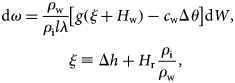
where the elemental volume of water dW is given by dW = QΔt, Q is the discharge, t is the time, ρw and ρi are the densities of water and ice, λ is the specific heat of melting ice, l is the length of the channel, g is the gravitational acceleration, c w is the specific heat capacity of water, Δθ = θ2 − θ1 is the temperature difference in the lake θ1 and at the exit of the channel θ2, H w is the water column depth, H r is the ice thickness and Δh is the drop in height along the channel length. The model assumes that the ice thickness above the channel does not exceed 200 m because it does not consider Glen's flow law. For example, a channel having a cross section of 1 m2 covered with 200 m-thick ice will have its cross-sectional area reduced to 1 million times (to 1 mm2) in 31 years. Thus, this approach is suitable for estimating the outbursts of lakes through an open channel or channel covered with a thin layer of ice.
To obtain more accurate ratios between ω and W we integrated Eqn (1) given the conditions corresponding to the glacial lake outburst flood's starting point and to a certain time t. Since the channel has not formed at the initial time, the lower limit of integration over its cross-sectional area dω is zero. W S is the volume of water in the lake at time t. This is the upper limit of integration concerning dW. Thus,
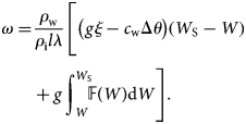
Let us turn now to the integral remaining in the right part of Eqn (2), and define of the tabular function $H_{\rm w} = {\opf F}( W)$ based on the depth measuring data. We use ${\opf S}( W)$
 to denote the result of numerical integration of arbitrary function $H_{\rm w} = {\opf F}( W)$
 at certain W. Then, we may write Eqn (2) as
If Q(ω, t) denotes the volume of water flowing through a cross section per unit time, the discharge, we may write the equation for this calculation as
where α is an empirical scale coefficient that is estimated based on the best fit between simulated and measured data. In the 1980s, Yu.B. Vinogradov and his colleagues performed physical experiments on ice-dammed lakes to determine the coefficient and solve various engineering problems. He also analysed the simulated and measured discharges for real outbursts of ice-dammed lakes. Thus, according to the collected data, the dependence of the scale coefficient α on the length of the ice channel was obtained. This dependence can be approximated by the relation lgα = −1.124×lgl + 0.7289 within an accuracy of ~2%, with l expressed in kilometres. So, α was determined based on the length of the channel, and also the dependence of the volume of the lake on the depth H(W), which was calculated according to the grid for all simulated scenarios.
The parameters that were embedded into the model were the grid of the lake water depths, the ice thickness, the temperature of the lake before the outburst flood, the channel's length and slope, and coefficient α. The constants for the simulation are specific heat capacity of water is 4190 J (kg °C)−1, its density is 1000 kg m−3, specific heat of ice melting is 3.34×10⁵ J kg−1, acceleration of gravity is 9.81 m s−2. The simulation results are presented in the form of a hydrograph of the outburst flood through a cross section at the end of the channel. As a result, we determined the distribution of water discharge over time, the diameter of the channel, the volume of the flood and the time of its termination for each outburst.
Results of field research
Boulder Lake and the supraglacial layer of water. First of all, we present the field results obtained in the study of Boulder Lake. Based on the data of the GPR sounding in January 2019, a complex vertical structure in the area of Boulder Lake was detected. The GPR time-section (Fig. 3) through the water body demonstrated this structure. The location of the profile is depicted in Fig. 1 as the blue thickened line (P1).
Weak (due to horizontal filtering) reflection 1 is the direct wave that corresponds to the ice surface. Intensive reflection 2 formed by a dielectric contrast boundary between the ice and the water-table of Boulder Lake. Since the reflection coefficient from 2 is very high, a number of multiple reflections 3 are also observed in the time-section. They are especially clear at the beginning of the time-section. Reflections 4 are related to the crevasses located in the ice above Boulder Lake. Reflections from the bedrock are shown by 5. The shoreline of Boulder Lake is marked by weak expressed diffracted waves 6. Reflection 7 indicates a thin lens of water on the ice of Boulder Lake. The depth of this lens was ~3 m. In addition, GPR revealed a layer of ice ~0.27 m thick above this supraglacial layer of water. On aerial photography, areas above it are reflected as local blue spots, prevalent mainly in the northern part of Boulder Lake. We present the described vertical structure in the form of a schematic block diagram (Fig. 4).
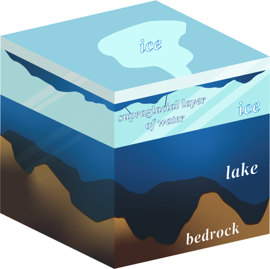
Fig. 4. Block diagram of the vertical structure of Boulder Lake and the supraglacial layer of water.
Unfortunately, we were unable to determine accurately the shoreline of Boulder Lake in the southern part due to the complexity of the wavefield on some GPR profiles and the insufficient density of these profiles. The lake therefore probably extended further to the south that we suggest (Fig. 5a). The lake is ~900 m in length, 450 m maximal wide and has a surface area of 195 000 ± 1000 m2. The lake basin has two elongate sections in the northern and southern parts, which narrow in the centre. In January 2019, a lake volume (water column) was estimated as 2 712 000 ± 15 000 m3. The maximum measured depth was 45 m with an average value of ~14 m. The ice thickness measurements vary from 2 to 18.5 m with an average value of 6 m (Fig. 5b). Ice thickness increases towards the southern and central parts of the lake, which are inland. The lowest values were detected near the rocks.
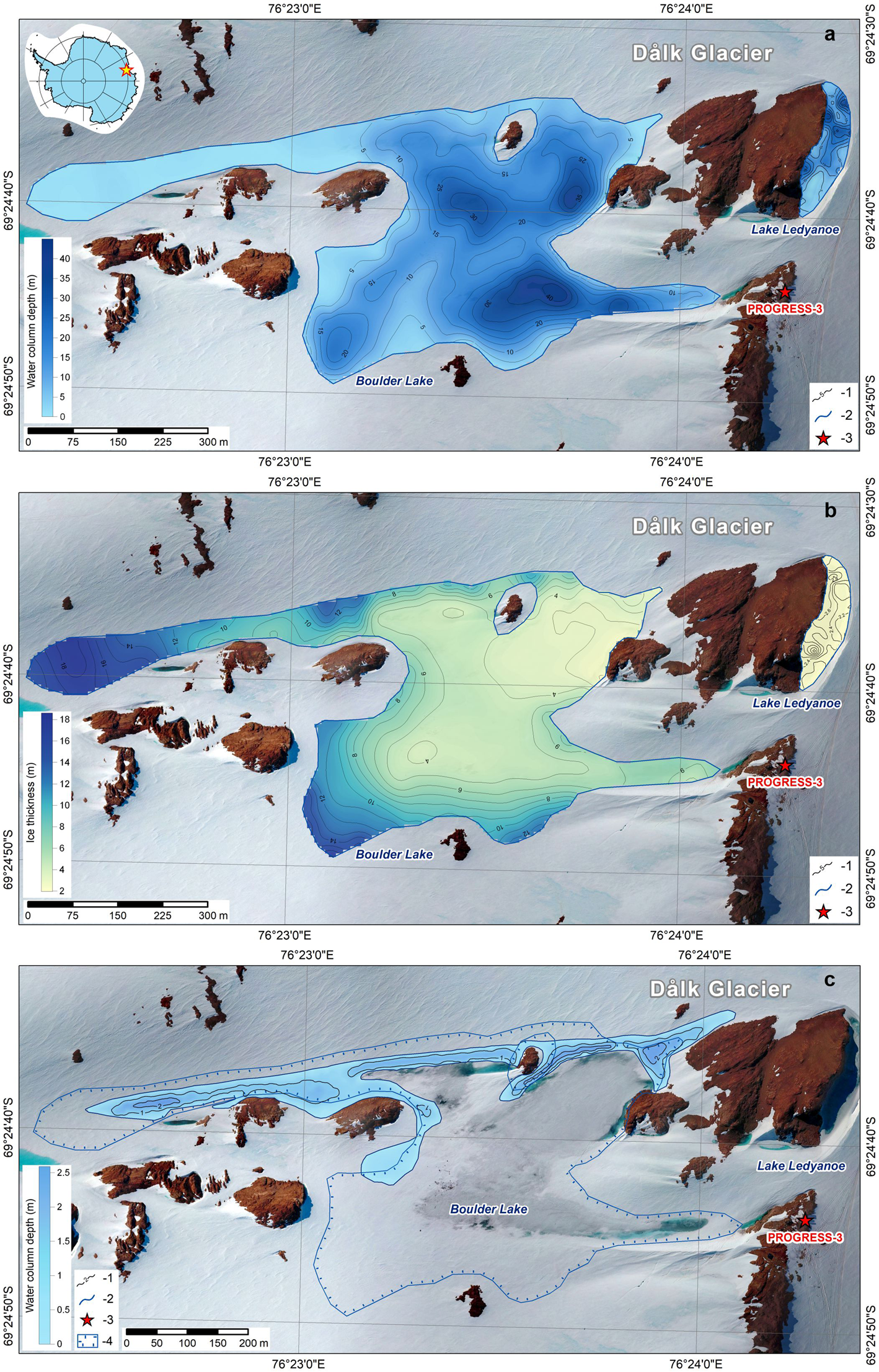
Fig. 5. Water column depths of Boulder and Ledyanoe lakes (a), the ice thickness over Boulder and Ledyanoe lakes (b) and depths of the supraglacial layer of water (c). (1) Depth contour (interval 5 m) (a), ice thickness contour (interval 1 m) (b), depth contour (interval 1 m) (c); (2) shoreline; (3) field base; (4) shoreline of Boulder Lake. The drone image by A.V. Mirakin in January 2019.
In 2019 we estimated the shoreline and morphometry of the supraglacial layer of water with high accuracy. The supraglacial layer is prevalent in the northern part of Boulder Lake and has a length of 1080 m and a width of ~50 m. According to the GPR results, this is a single layer of meltwater, which is characterised by an area of ~40 000 ± 200 m2 and a water column volume of ~40 240 ± 200 m3. The bathymetric scheme of that layer is shown in Fig. 5c. The maximum water column depth of the supraglacial layer of water is 2.9 m, and the average depth value is 1.1 m. The ice thickness above has a value of 0.27 m and distributes uniformly. We do not know exactly what configuration and volume the supraglacial layer of water had before the 2017 outburst flood. Nevertheless, in further modelling, we assume that the volume of the supraglacial water layer was similar to that measured in 2019. This is the basic assumption when calculating the outburst into Lake Ledyanoe. Two-year observations of the water level of Boulder Lake during the field seasons allowed us to describe its summer dynamics. In January 2018, we registered the rise of the lake's water level, which was caused by an influx of seasonal meltwaters. We observed the same trend in January and February 2019. Noteworthy that the water level in the lake was 70 cm higher than in 2018. Considering the outburst nature of the water body, we can conclude that it was in the stage of filling. Boulder Lake was permanently ice-covered during the 2-year study period, and the water temperature at a depth of 0.2 m from the surface did not exceed 1–2°C.
Lake Ledyanoe. Lake Ledyanoe has a hook shape. The lake is ~220 m in length, and 50 m maximum wide. According to the results of the GPR sounding, which we completed on 25–26 of January 2019, the lake area is 8900 ± 45 m2, and the lake volume is 125 500 ± 600 m3. The maximum measured depth of the water column was 39.7 m with an average value of ~14.1 m (Fig. 5a). The measured ice thickness above the lake varies from 2 to 3.6 m. The maximum value is observed from the rock's side (Fig. 5b).
The observations of the water level of Lake Ledyanoe in January–February 2018 showed a decrease in the level by 5 cm. Most likely, the decreasing trend remained till January 2019, because the water level dropped below the zero of gauge. However, we cannot indicate the precise value of the water level decrease (not <0.5 m). At the same time, surface runoff was not detected. Thus, perhaps the lake water drained through crevasses in the glacier. Moreover, in 2019, we found the indicators of the flood of 2017. Those were detected on the glaciated bank of Lake Ledyanoe as prints of the maximum lake water level prior to the outburst. The absolute height of that level was 102.4 m. We calculated the volume of the basin based on the present topography to estimate the volume of Lake Ledyanoe before the outburst. The calculation was limited to 102.4 m. Therefore, we obtained the maximum depth of Lake Ledyanoe before the outburst as 43 m, and its water volume as 164 600 ± 800 m3. The linear size of the water body also remained unchanged. Measurements of the temperature of the water layer at a depth of ~0.1 m showed that it did not exceed 1–2°C.
Lake Dålk. We were able to estimate the conditions of Lake Dålk before it drained using the GPR sounding completed during 58th RAE (2012/13) (Popov and Eberlein, Reference Popov and Eberlein2014). The GPR time-section and its approximate position are presented in Fig. 6. In addition, the location of the route is shown in Fig. 1 as the yellow line (P2). The direct wave on the time-section is almost invisible due to the use of horizontal filtration. The position of the direct wave corresponds to the zero value on a vertical axis. Reflection 1 is formed by the water table of the lake. Reflection 2 is represented as multiple waves, which were also formed by that surface. According to the travel-time curves of the two diffracted waves 3 a permittivity value of 2.6, was estimated. This is a typical value for a snow-ice mass, which was obtained on the glaciers in the areas of the Progress and Mirniy stations, East Antarctica (Popov and others, Reference Popov, Polyakov, Pryakhin, Mart'yano and Lukin2017a; Sukhanova and others, Reference Sukhanova, Popov, Boronina, Grigorieva and Kashkevich2020). The upper layer is represented as a snow-ice mass with a thickness of 14.3 m at the profile beginning, ~9.5 m in the area of diffracted wave and 10.5 m on the right boundary of layer 2. The reflections from the bottom of Lake Dålk are not observed on the time-section. If we suppose that the bottom position is the same as it was before the 20-m depression had formed, then the reflection from the bottom should be situated on delays ~1400 ns. This exceeds the size of the recording interval by almost three times. The contrast reflection 4 represents a boundary between the snow-ice mass and the bedrock. The most challenging part was the interpretation of area 5, which is located in the central part of the time-section. The mosaic structure of the wavefield and absence of the reflection in the deep part of 5 suggests it could be a very dissipating media. We tend to think that it could be watery snow slush or other media with similar properties. The thickness was determined in accordance with the dielectric constant of 3.17 (Macheret, Reference Macheret2006). Reflection 6 over area 5 corresponds to ice ~0.5 m thick.
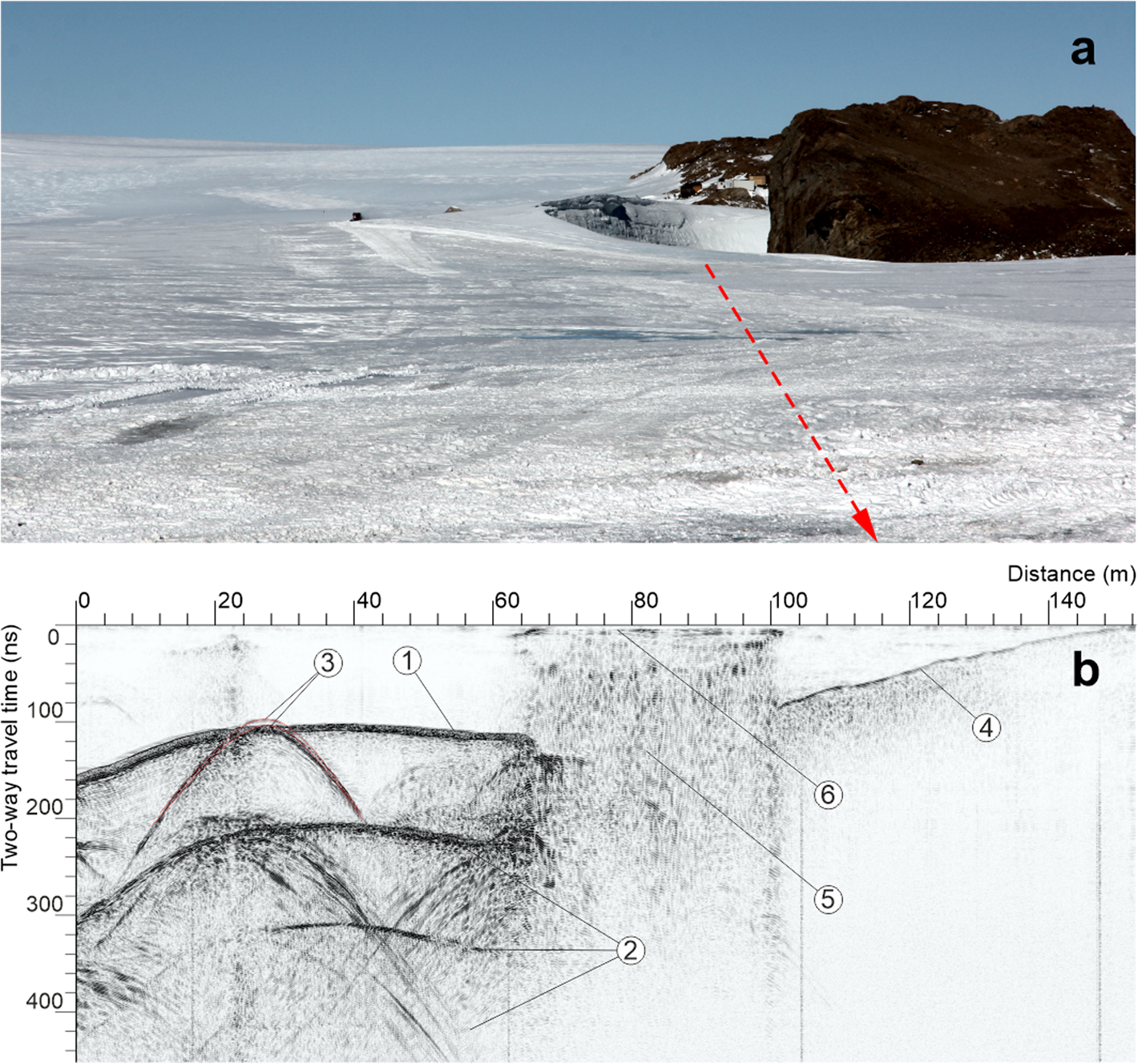
Fig. 6. Photo (a) and GPR time-section (b) collected in February 2013 in the western part of Lake Dålk. (1) Reflection from the water-table of the englacial water reservoir; (2) multiple reflections from the water-table; (3) diffracted waves; (4) reflection from the ‘ice–bedrock’ interface; (5) wet snow layer; (6) reflection from the ‘ice–wet snow’ interface. Photo by S.V. Popov in February 2013.
Drainage channels. Another purpose of our fieldwork was to find drainage channels formed during the outburst. According to the photos and videos taken at the time of drainage in 2017, an open channel was observed between the Boulder and Ledyanoe lakes (Fig. 7a). In January 2017 an investigation into the structure of the surface stratum was not carried out. Nevertheless, we assume that seasonal snow did not accumulate, but melted on a warm Austral summer day, seeping into the firn layer and provoking its watering and partial melting. This meltwater froze during the cold summer night. Such a cyclic process of metamorphism turned the snow-firn layer into a porous medium, similar to ice, but with a reduced density of ~800 kg m−3. The assumption of intense snow melting is supported by the information that the Austral summer 2016/17 was relatively warm. According to the Progress meteorological station, the average temperature in December 2016 and January 2017 was +1°C, and the maximum temperature reached +8.1°C. Although in the previous 10 years, the maximum temperature in January–February mainly varied in the range from +4.5 to +5.5°C. Probably, the drainage channel between the Boulder and Ledyanoe lakes was formed in the porous ice-like strata.

Fig. 7. Drainage channels: (a) from Boulder Lake, (b) between the Boulder and Ledyanoe lakes, (c) channel inlet to depression and (d) photo locations from sections (a–c) and Figure 14. Photos by A.V. Mirakin, 30–31 January 2017.
In January 2018, we studied the area between the Boulder and Ledyanoe lakes. During the research, we identified the channel formed after the 2017 outburst from GPR. GPR time-section is depicted in Fig. 8. The location of the route is shown in Fig. 1 as the green thick line (P3). The direct wave which also is the surface is pointed by 1. Reflection 2 relates to the bedrock. The contrast diffracted wave 3 is formed by the bottom of the channel. The high intensity of this reflection is due to the smooth channel walls, polished by the water flow in 2017. The reflectivity of the boundary between ice formed from melted water and environmental firn-icy media is relatively high. The diffracted wave 4 is also associated with the channel. This wave is formed by its roof, which is connected to the surface of 2017. The high intensity of this reflection is explained with the same reasons as for wave 3. Intensive reflection 5 is also related to the surface of 2017, formed by the end of the warm period. A small part of outburst water could seep to the surface, then frost and form a dielectric contrast boundary. During autumn, winter and spring it was covered by snow which was transformed into icy media by metamorphic processes of melting and refreezing during the warm summer period of 2017 and 2018. As mentioned above, the surface strata were formed as a result of the freezing of meltwater and had a permittivity of ~2.6. This volume was measured along the time curve formed by crevasses (Sukhanova and others, Reference Sukhanova, Popov, Boronina, Grigorieva and Kashkevich2020). Based on the permittivity of 2.6, the depth of the channel roof is 2.8 m, and the diameter of the channel is 1.2 m.
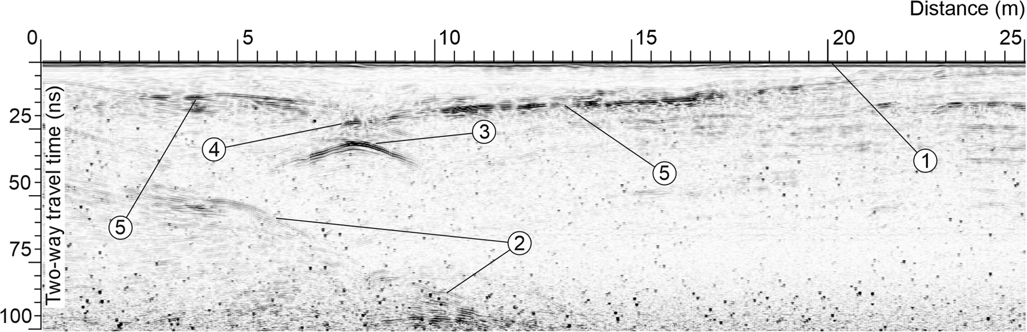
Fig. 8. GPR-time section in the area near Boulder Lake. (1) Direct wave; (2) reflection from the bedrock; (3) bottom of the englacial channel; (4) roof of the channel; (5) reflection related to the surface of 2017.
After the water from Boulder Lake had merged with Lake Ledyanoe, it flew to Lake Dålk. Initially, the water was moving in an open channel, but at ~150 m from Lake Ledyanoe, water had seeped into the glacier through the crevasses and formed an englacial channel. The expedition staff who observed this outburst confirmed that the water drained to Lake Dålk not on the surface, but inside the glacier (Fig. 7b). The positive air temperatures indicate that the thickness of snow was insignificant. In January 2018, we drilled 2 boreholes in the area between Lake Ledyanoe and the depression for the retrieval of ice cores. The boreholes were 0.9 and 3.6 m deep. The measured density showed similar values (Fig. 9). This is due to the homogeneous structure of the glacier. In core 1, firn with a density of ~825 kg m−3 was observed to a depth of 20 cm, while the ice was detected deeper than that point. This compaction in the near-surface layer is most likely related to weather conditions. Core 2 was a block of monolithic ice with interspersed air bubbles. We assume that there was a similar glacier structure in January 2017, and the drainage channel was located inside the ice. The water flow between Lake Ledyanoe and the depression was identified from the photos taken during the 2017 outburst. However, after modelling the water flowlines, we were able to identify the path of the water discharge from Lake Ledyanoe to Lake Dålk more accurately. In Fig. 10 it is visible, the simulated stream goes around the rock outcrop near the field station Progress-1 from the eastern side and enters the englacial reservoir on the southeast. The modelled position of the channel is in good correlation with the photos and video records, which were taken during the outburst flood in 2017.
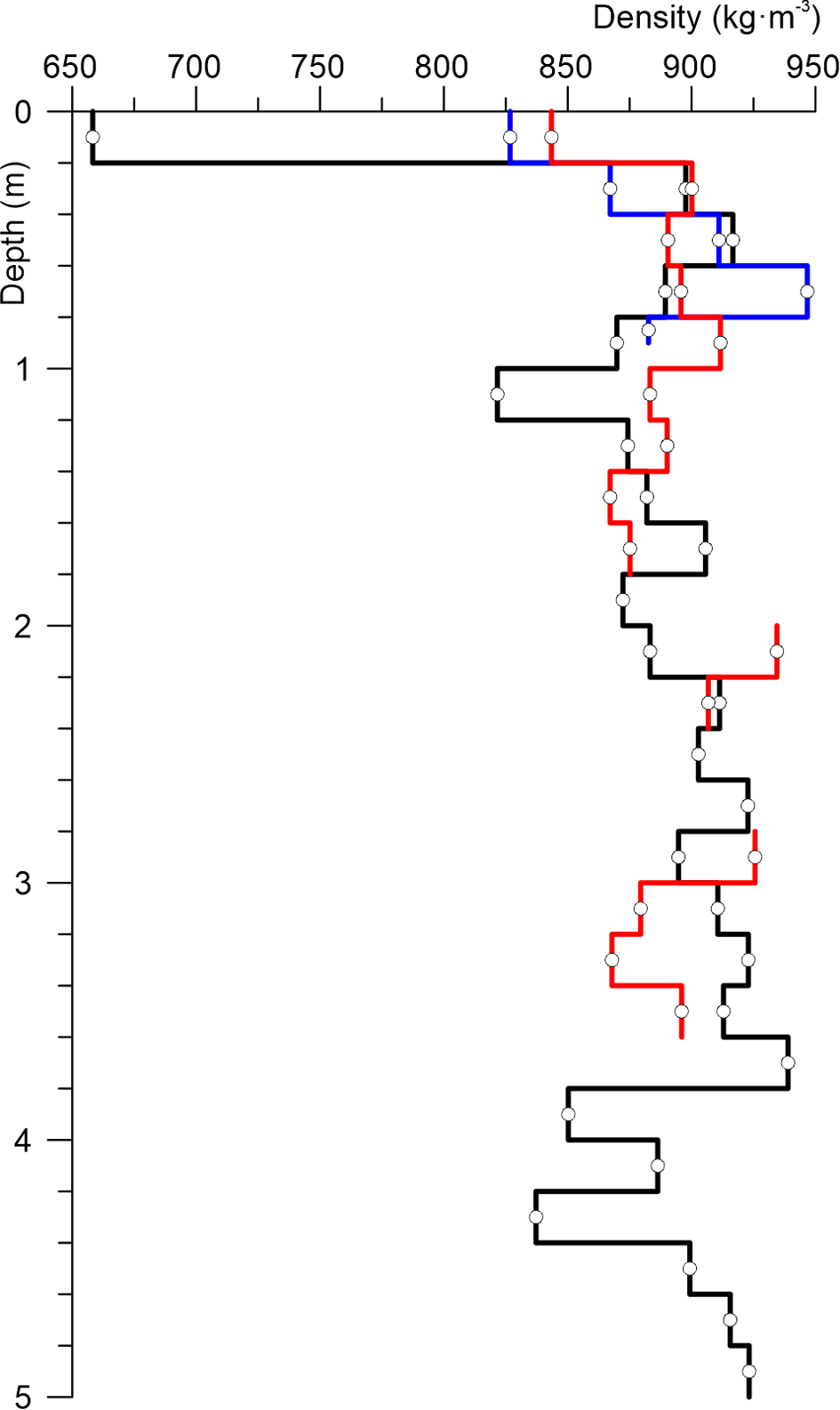
Fig. 9. Cores densities from boreholes: (1) blue line; (2) red line; (3) black line.
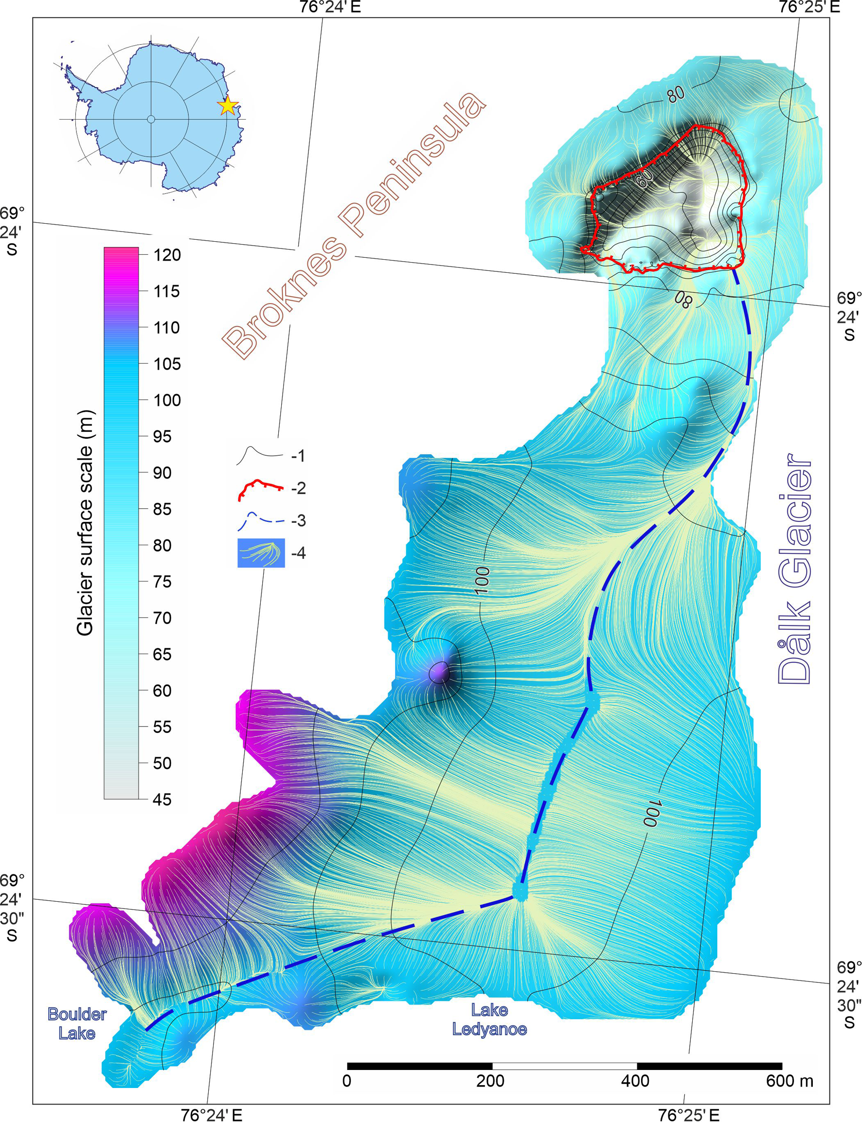
Fig. 10. Ice surface elevation map in the area between the depression and lakes. (1) Ice thickness contour (interval 5 m); (2) the boundary of the depression on 8 January 2018; (3) englacial channel; (4) flowlines.
The flow of water entered Lake Dålk through the englacial channel and formed the cave shown in Fig. 7c. The Lake Dålk basin consisted of ice. This is confirmed by visual observations inside the depression and by the structure of 5 m core sample taken near it. The entire layer to a depth of 5 m, except for the first 20 cm, was monolithic transparent ice. In addition to transparent ice, granular ice formed by recrystallisation has also been observed. The core density distribution is shown in Fig. 9. There was no surface outflow of water from Lake Dålk during its outburst. The water was certainly drained from the pond through an englacial channel. However, we did not detect the drainage channel by GPR sounding the year after the flood (in January 2018). There are two reasons for explaining that. First, according to the observation results from the glaciological stakes, it was discerned that the flow velocity of Dålk Glacier in the area of the depression are significant and had values of 2–3 m in the period from 17 January to 22 February 2019. Presumably, the channel disappeared due to the glacier's displacement. Second, we may not have found the channel on the GPR time-section because of the abundant number of crevasses surrounding the formed depression. They can blind the reflection from the channel.
To sum up, we collected all the necessary information to describe the mechanisms and to create the phenomenological description of the outburst of 2017. Moreover, all of the field data served as initial conditions for the outburst model.
Discussion
The phenomenological description of the outburst
We present a phenomenological model of the lake's outburst in 2017 based on the results of field research. The model is shown as a block diagram in Fig. 11.
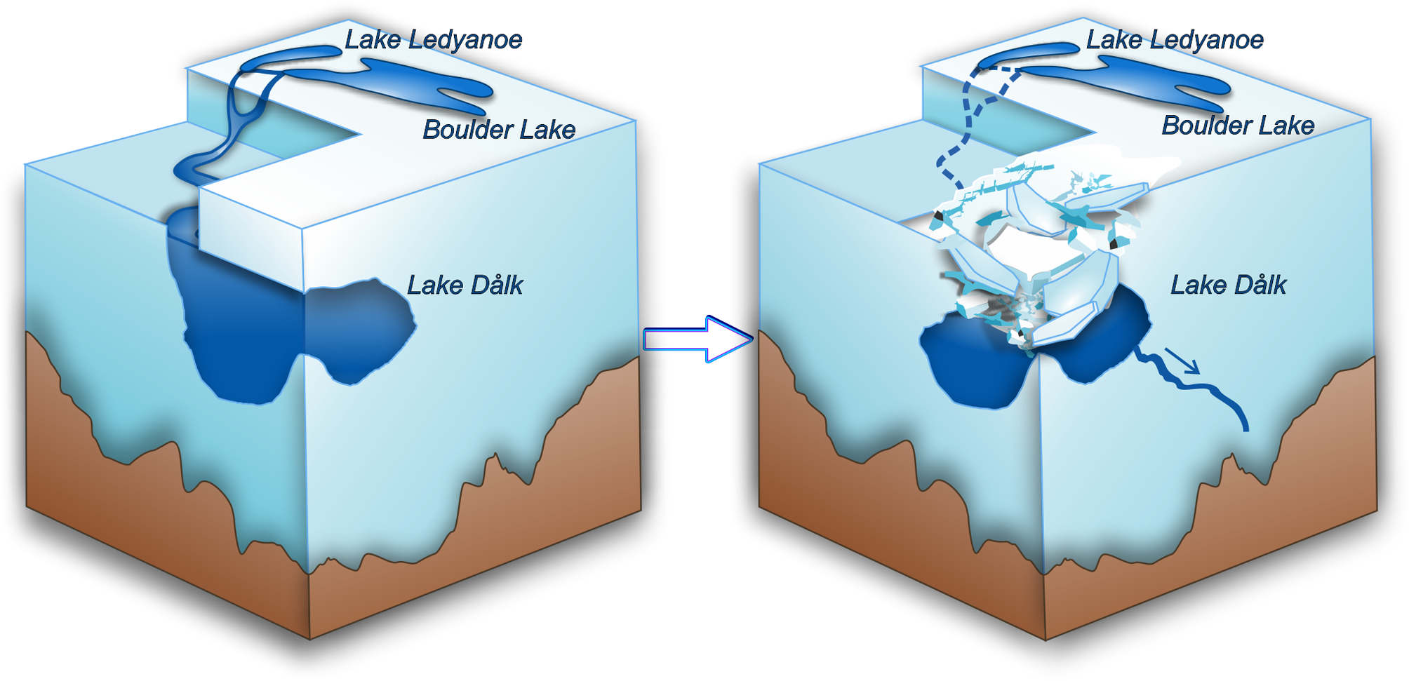
Fig. 11. Block diagram of the outburst flood and the formation of the depression on Dålk Glacier.
We suppose that the outburst of the hydrological system began with the overflow of the supraglacial water layer in the Boulder Lake area. We make this assumption based on two pieces of evidence. First, the video recorded during the flood clearly shows that the drainage channel begins precisely from the supraglacial water layer located on the ice of Boulder Lake. Second, during the fieldwork of the 63rd RAE, a year after the outburst, we found traces of destroyed ice at the site of the former supraglacial layer of water. We believe this ice covered the water and then collapsed when it drained. If Boulder Lake had depleted in January 2017, we would have found a subsidence of ice covering this water body. However, this did not happen. Thus, there is every reason to assert that it was the overfill of the supraglacial water layer that was the beginning of the outburst of the lakes system. The main source of water for the formation of the supraglacial lens on the ice surface of Boulder Lake was the melted snow of the surrounding rocks and the glacier. We used two drone images from January 2017 (just before the drainage) and January 2019 to compare the supraglacial layer of water configuration as it makes the ice look blue at the surface. In general, the size of the supraglacial layer of water in 2017 was 10% greater than one observed in 2019. Probably by 2019, as a result of the melting seasonal snow and ice, the supraglacial lens began to recover and return to its previous size. Unfortunately, we do not have satellite or drone images immediately after the 2017 outburst to estimate the size of the supraglacial layer of water back then.
The discharged flow from the supraglacial layer of water partly entered Lake Ledyanoe as well as flowed towards Lake Dålk. The volume of water from the supraglacial lens filled the basin of Lake Ledyanoe to the high-water elevation by the morning of 29th January 2017. On that day, the outburst of Lake Ledyanoe began. As mentioned earlier, during fieldwork, we found indicators of the lake water level prior to the outburst on the glaciated bank of Lake Ledyanoe. The absolute height of that level was 102.4 m. Based on that value, we assumed that the ice dam is capable of storing a mass of water, up to a height of 102.4 m. If this value is exceeded, the water will overflow, as happened during the 2017 drainage event. The lake was discharged through the ice dam as an overflow. The dam did not collapse. According to our estimates, the volume of water that entered Lake Ledyanoe was 39 120 ± 200 m3. Thus, Lake Ledyanoe had accumulated almost the entire volume of the supraglacial layer of water. Having escaped out of it, the water began to move towards the Prydz Bay. The flow moved both along the glacier surface in the channel and passed into glacial crevasses (Fig. 7b). According to the video recordings, the rapid flow of water from Lake Ledyanoe continued until 31st January 2017.
The volume of water entered Lake Dålk and threw it out of equilibrium (Fig. 7c). The reservoir water level increased until it reached a critical stress, which triggered it drain englacially. The first ice subsidence happened on 30 January 2017. However, on 31 January, there was a second outburst from Lake Dålk, and the depression increased to a huge size. We understand that this is only a phenomenological description, but in our opinion, it is close to reality. In the next section, we present the results of mathematical modelling of the lake's outburst flood.
Modelled outburst flood of the lakes system
The outburst of the supraglacial layer of water near Boulder Lake. We estimate the outburst of each of the three lakes sequentially, as described in the phenomenological model. First of all, we simulate the characteristics of the flood during the drainage of the supraglacial layer of water. We are using the model described in section ‘Model to estimate lake outburst floods’ (Popov and others, Reference Popov, Pryakhina and Boronina2019). Primarily, we must define the maximum volume of the supraglacial lens. These data are needed for calculating the bathygraphical curve. Based on field results, the maximum volume of the supraglacial layer of water was 40 240 ± 200 m3. The water temperature is assumed to be 1.5°C since a shallow layer of water can warm up to hotter than 0°C in the summer. In addition, we relied on data on water temperature in ice-covered lakes obtained during the field seasons (2017/19). Their water temperature values changed from 1 to 2°C. For calculation we used the average value. Water drainage began through the channel formed in a porous medium, similar to ice, but with a reduced density of ~800 kg m−3 in the northeastern part of Boulder Lake. The length of this channel was ~180 m with a maximum diameter of 1.2 m. The drop in height along channel length was 4.13 m. In January 2017, the supraglacial layer of water was covered with ice. We assume its thickness varying slightly from year to year and is on average equal to the value we measured in January 2019. The ice thickness was 0.27 m. The calculation also requires setting several constants. They are defined in the ‘Methods’ section, except for the dam density taken as 800 kg m−3. The calculation results are shown in Fig. 12. Analysing the flood hydrograph, it can be seen that the curve changes smoothly, without sudden changes in discharge. It took 27.5 h for the water from the supraglacial layer of water to fill Lake Ledyanoe to the high-water elevation. We do not know certainly how long the water flowed out of the supraglacial layer of water. Nevertheless, the expedition staff who observed this process estimated its duration to be about a day. The maximum discharge was 0.92 m3 s−1 and was reached 21 h 10 min after the beginning of the emptying of the supraglacial layer of water. The calculated value of the channel diameter correlates well with field measurements. The results of the GPR sounding of 2018 showed that the diameter was 1.2 m. The calculation results showed that the diameter was 1.28 m. The error is ~10%. However, the field study was carried out a year after the outburst, so the channel bed could be deformed by this amount. The maximum diameter was reached by the end of the flood. This is logical because the water flows thermally incised the channel throughout the entire drainage (Fig. 12b).
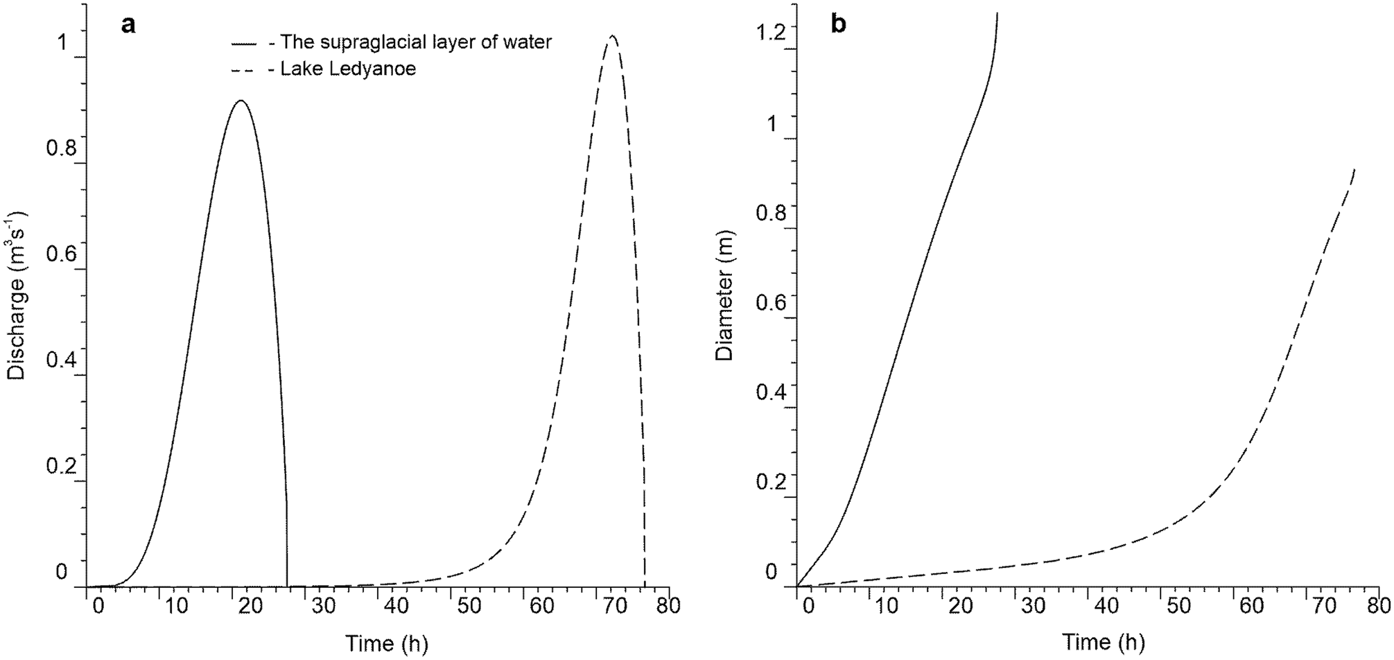
Fig. 12. Simulated hydrographs of the outburst floods (a) and channel diameters (b).
The outburst of Lake Ledyanoe. The volume of water from the supraglacial lens filled the basin of Lake Ledyanoe to the high-water elevation by the morning of 29th January 2017. On that day, the outburst of Lake Ledyanoe began. The volume of water equal to 39 120 ± 200 m3 was used for the formation of the flood from Lake Ledyanoe. We determined this value, knowing the high-water elevation of the reservoir and its volume before emptying. At the same time, the volume of water that was discharged from the supraglacial layer of water (40 240 ± 200 m3) and which entered Lake Ledyanoe (39 120 ± 200 m3) is in good agreement. Probably, the missing 1120 ± 6 m3 of water flowed immediately towards Lake Dålk. The length of the englacial channel connecting the Ledyanoe and Dålk lakes was ~1240 m. We have shown the channel position in Fig. 10. According to tacheometric measurements, the drop in height along channel length was 26.9 m. The water temperature was assumed to be 1.5°C, consistent with the previous model case. Unfortunately, this is our assumption, since the exact value is not known. The thickness of the ice equals zero because the water surface did not have time to be covered with ice. The constants are the same as the previous model, except for the density of the medium surrounding the englacial channel (900 kg m−3). The calculated hydrograph has an asymmetric shape (Fig. 12a). Its gentle rise ends with a sharp decline and the cessation of the process. Water discharge did not exceed 0.1 m3 s−1 for the first 2 days. Then a noticeable increase in the power of the water flow began. The maximum water discharge was reached on the third day, after 72 h and 10 min from the start of the drainage. It was ~1.05 m3 s−1. In total, the drainage of water lasted 76.5 h. According to the information from the expedition staff, the flood lasted for ~2.5–3 days (29–31 January). Unfortunately, we have only such indirect data to assess the correctness of the calculated characteristics.
The channel connecting the supraglacial layer of water and Lake Ledyanoe expanded rapidly. Its diameter increased smoothly and almost linearly. The tendency of the channel evolution connecting Lake Ledyanoe and Lake Dålk differs from the aforementioned one. As can be seen in Fig. 12b, the expansion of the englacial channel was slow. The inflection in the graph is associated with a sharp rise in water discharge. The maximum diameter of the englacial channel was ~1 m. Thus, the development of the open and englacial channels occurs in different ways, and their length also plays a key role.
The outburst of Lake Dålk. We suggest that the outburst of Lake Dålk was through a moulin at the base of the lake. According to airborne radar data obtained during the fieldwork of the 36th Soviet Antarctic Expedition (1990/91), the thickness of Dålk Glacier at the latitude of the dip was ~800 m (Popov and Kiselev, Reference Popov and Kiselev2018). According to the Antarctic Digital Database (ADD, Reference ADD2016) Dålk Glacier is an ice shelf. Thus, knowing the average thickness of the glacier and the depth of the depression, we calculated the height difference between the beginning of the channel and its end. The estimated height value was 764 m. We were forced to estimate several scenarios for the outburst of Lake Dålk since no runoff channel was found. The channel lengths were: 764, 821, 971 and 1134 m. The smallest of the values (764 m) corresponds to the outflow of lake water along the shortest distance under an ice shelf, like a waterfall. The largest value corresponds to the movement of water through Dålk Glacier to the Prydz Bay. A bathymetric chart of the englacial reservoir before its emptying was drawn from the tacheometric survey carried out in 2018, taking into account snow accumulated during 2017 (Boronina and others, Reference Boronina, Popov and Pryakhina2018). Since Lake Dålk was completely empty in January 2017, the flood volume was 708 700 ± 3500 m3. There were no data on the water temperature in the lake. We assumed it to be ~0°C, because the water body was completely covered by ice. The thickness of the ice above the lake was 4 m. We estimated this value from the collapsed ice roof. The calculated hydrographs are shown in Fig. 13a.
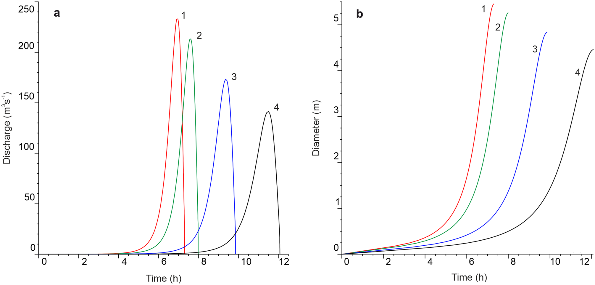
Fig. 13. Simulated hydrographs of the outburst of Lake Dålk (a) and channel diameters (b). Channel lengths: (1) 764 m; (2) 821 m; (3) 971 m; (4) 1134 m.
The simulated hydrographs of the Lake Dålk outburst are characterised by a negative asymmetry. The largest water discharge was obtained with the channel length of 764 m. This maximum discharge was 230 m3 s−1 and was reached 6 h 57 min after the start of emptying. The flood intensity dropped sharply after the peak, and after ~25 min, the outburst stopped. The hydrographs are characterised by a gentle rise and a sharp decline in all design scenarios. The outflow time to the Prydz Bay was ~12 h. The maximum water discharge was reached after 11 h 27 min and amounted to 141 m3 s−1. The channel diameter is minimal at the beginning of the outburst and is maximum by the end of it. Also, on the graphs (Fig. 13b), it can be seen that from a certain moment, the value of the diameter begins to increase. The speed at which this inflection point occurs depends on the water discharge.
Thus, the drainage of Lake Dålk and the subsequent formation of the depression is the final stage of the above-described process. Unfortunately, we cannot compare the simulation results (Fig. 13) with real observations due to their absence. Since no moulin from the lake was detected, we had to examine several designed cases considering different lengths of the channel: from the shortest one that is vertically down under the glacier, to the longest one – to Prydz Bay. We find it difficult to suggest which option is the most suitable since we have eyewitness information only about the stages of depression formation. However, the process of destruction of the ice roof over Lake Dålk, which took place at the initial stage, was not related to the outburst but was associated with the intensive inflow of water from Lake Ledyanoe. We believe that the overpressure caused by the overfill of the lake led to the collapse of the ice roof, and further, to the drainage of Lake Dålk. At the same time, the eyewitnesses combine these two events that do not allow us to properly assess even the duration of the drainage. A review of the results obtained on modelling the outburst of three lakes and the input data are presented in Table 1. For the case of the englacial reservoir, data on the drainage to the Prydz Bay are given.
Table 1. Input data into the model and obtained result
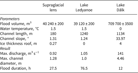
Summarising the results of all simulations, we believe that the main inaccuracy in the assessment of the outbursts’ characteristics was introduced by the lack of data on water temperature in the lakes before drainage. We suppose that an assumption to take 0°C for Lake Dålk is not significantly wrong, since it was an englacial reservoir. Nevertheless, in the supraglacial lens and Lake Ledyanoe, the water temperature could be higher than we assumed. In such a case, it would lead to faster drainage and higher discharges. Another factor influencing the simulation results is the density of the medium through which the water flows out. We believe that all used density values are justified and confirmed by cores. All other input data were obtained in the field and should not have introduced a large error in the calculation results. We suggest that the complete outburst of the lake system occurred in the same time interval as obtained from the simulation results.
New outburst of the lakes system
The behaviour of such active lakes is characterised by several stages: water accumulation, overfill, dam breakage or overflow, drainage of excess water and stability before the next overfill. In such a manner, we can suppose that the outburst cycle begins with the lake's overfill and ends with its following overfill. The next overfill and drainage of the described lakes’ system took place in January 2020. In general, the outburst had a similar scenario, but there were some differences. Similar to 2017, the first reservoir to overflow was in the Boulder Lake area. However, on 8th January 2019, water began to drainage not only from the supraglacial layer of water but also from Boulder Lake. We registered a decrease in the water level of the lake. Water drainage was in the form of two streams. The water flowed into Lake Ledyanoe and accumulated on its ice surface for 2 days. On 10th January 2020, there was an overflow of water from Lake Ledyanoe. A channel with an average width of 1.3 m and the maximum depth of 0.35 m was formed in the glacier. Moving towards the depression, water flowed in the channel as well as passed into glacial crevasses. During the day, the outburst flow of water from Lake Ledyanoe reached the depression and began to fill it intensively. The depression filled to the brim in 14 days. One would expect that after the reappearance of Lake Dålk, its outburst would follow the scenario of 2017, however, it did not. Lake Dålk began to flood in the northeastern part towards the Prydz Bay, and in the western part towards the Progress-1 field base (Fig. 14a, b). The stream directed towards the ocean was originally a narrow channel and then branched out and expanded. The water flow was no longer visually observed at a distance of ~400 m from Lake Dålk. Probably, water drained into ice crevasses. Drifting snow on the Broknes Peninsula in the first days of February 2020 filled the Boulder and Ledyanoe lake channels with snow causing the water to freeze. On the same days, Lake Ledyanoe and Lake Dålk were covered with ice (Fig. 14c).
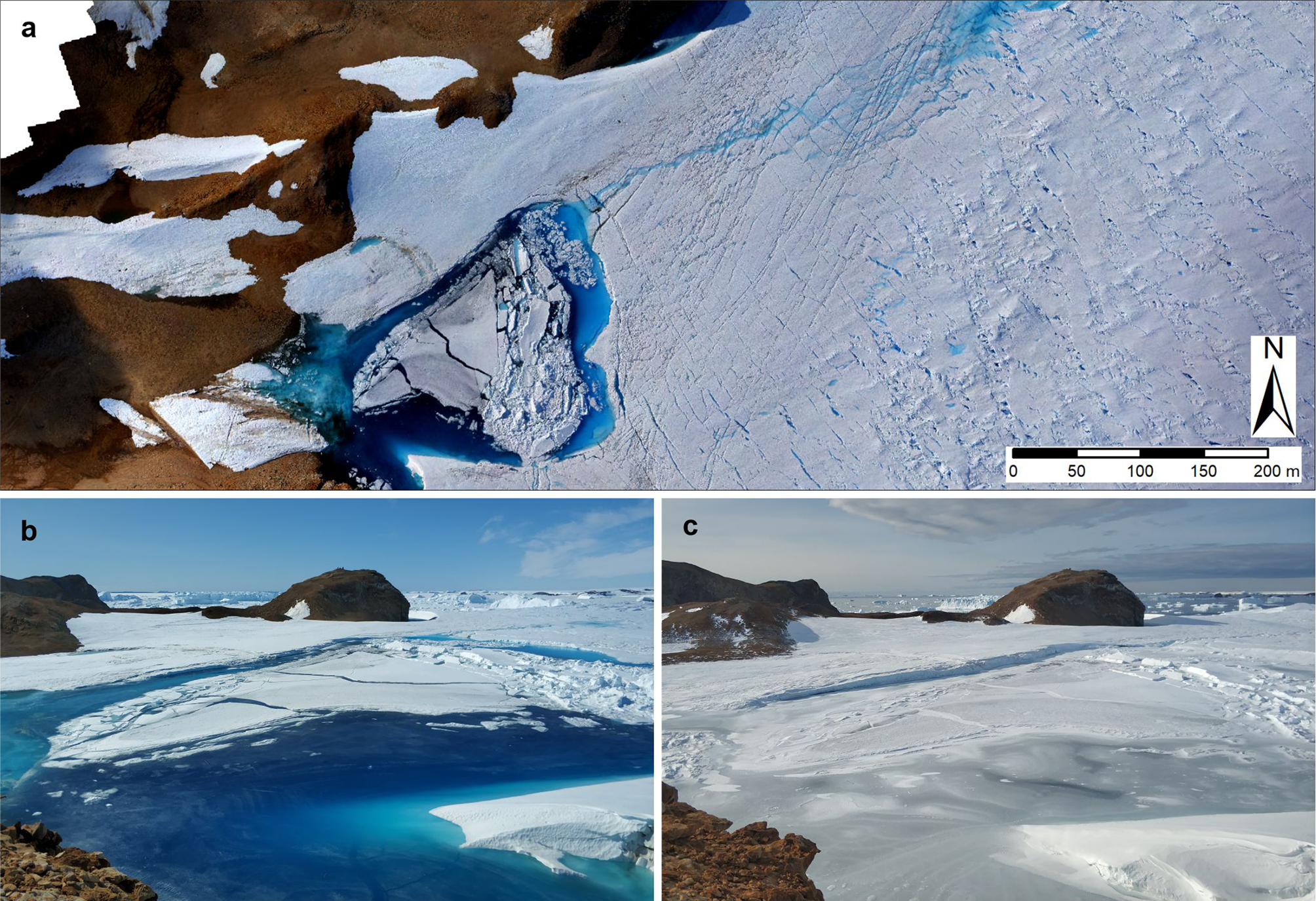
Fig. 14. State of Lake Dålk in 24–25 January and 3 February 2020. The stream from the lake directed to Prydz Bay (a); overcrowded lake (b); frozen Lake Dålk (c). Drone image by S. Grigoreva, 25 January 2020.
Based on the new data, we do not exclude that the water from Boulder Lake could have been involved in the formation of the flood in 2017. Nevertheless, in 2017 the whole process was not long and, probably, the contribution of Boulder Lake is insignificant. We believe that the proposed phenomenological description and the results of mathematical modelling do not contradict reality. Lake Dålk will empty similarly to the scenario of 2017 if it becomes englacial again.
Conclusion
The results of 3-year field research, combined with mathematical modelling, allowed us to create the phenomenological description of the process and estimate the outbursts of the Boulder, Ledyanoe and Dålk lakes. We have calculated hydrographs, changes in channel diameters and total flood times. We found that the reason for the lakes’ system outburst in 2017 was the emptying of the supraglacial layer of water. The series of calculations carried out for the drainage of Lake Dålk confirmed that it was the most powerful flood that led to the formation of the depression as a result of ice-sheet subsidence. The calculated characteristics of the outburst (water discharge, channel diameter and outflow time) are in good agreement with the field observations data, in particular, with the results of GPR sounding. The model used has shown its suitability to describe the drainage of this genesis.
Acknowledgements
We thank Russian Antarctic Expedition headed by A. Klepikov for providing logistics and G. Deshevih, E. Kiniabaeva, M. Kuznetsova, A. Mirakin and A. Sukhanova for help in the fieldwork. We are grateful to Dr P. Fretwell and D. Amaro Medina for the corrections and suggestions for improving English, also Dr A. Zirizzotti and Dr S. Urbini from the National Institute of Geophysics and Volcanology, Rome (Istituto Nazionale di Geofisica e Vulcanologia, INGV) for equipment provided for our fieldwork in 2012/13. We thank Dr S. Livingstone and an anonymous reviewer for thorough reviewing, which greatly improved the manuscript. This scientific work was supported by the Russian Foundation for Basic Research grant No. 18-05-00421.


 Open access