


Key points
• Record of ice temperature profile was retrieved through the use of autonomous data loggers.
• While the growth rates (μm s−1) of pond ice decreased, the temperature record demonstrated that the cooling rates near the ice–water interface (°C s−1) increased.
• Gas bubble layers formed during the high growth rates of ice.
• Water to ice heat flux and presence of gas bubbles within the ice and in the vicinity of the ice–water interface control the ice growth rate.
1. INTRODUCTION
1.1 Growth and thickening of lake ice
As water in a pond/lake cools from above 4°C, the surface water loses heat, becomes denser and sinks. This continues until all of the water in the pond/lake is at 4°C, when the density of water is at its maximum. Further cooling (and no mechanical mixing) will make a stable, lighter layer of colder water along the surface. As it cools to the freezing point, ice begins to form (Ashton, Reference Ashton1986).
Once an initial layer of ice has formed at the pond/lake surface, further growth continues in proportion to the rate at which energy is transferred from the bottom surface of the ice layer to the air above (Ashton, Reference Ashton1986). The growth of ice due to the heat loss from the ice has been traditionally treated as 1-D and vertical. The large vertical temperature gradient represents much greater vertical than horizontal heat flux (Leppäranta, Reference Leppäranta1993; Ashton, Reference Ashton2011).
Ice grows mainly at the bottom of the layer of ice as latent heat released due to freezing is conducted upward through the ice (Mullen and Warren, Reference Mullen and Warren1988; Leppäranta, Reference Leppäranta1993) and released to the air/snow above. Heat loss from the surface of the ice to the air occurs by a variety of processes, including conduction and radiation (Ashton, Reference Ashton1986; Leppäranta, Reference Leppäranta1993). Because the thermal conductivity of ice is 1–2 orders of magnitude larger than that of snow (compaction, humidity dependent), any thickness of snow over ice provides a thermal barrier between the air and the ice. The thickness of the ice over ponds or lakes depends, therefore, on how much snow covers the pond/lake (Adams and Roulet, Reference Adams and Roulet1980).
A pond/lake exchanges heat with the atmosphere above and with the sediment below. When ice cover is present heat flows from the sediment to the water and from the water to the ice (Ellis and others, Reference Ellis, Stefan and Gu1991). Without significant water motion and mixing, due to the absence of surface wind shear, the heat transfer from water to ice is mainly diffusive (Malmberg and Nilsson, Reference Malmberg and Nilsson1985; Ellis and others, Reference Ellis, Stefan and Gu1991). There is a thin laminar boundary layer just below the ice, where the molecular properties of water determine the heat transfer (Malmberg and Nilsson, Reference Malmberg and Nilsson1985; Ellis and others, Reference Ellis, Stefan and Gu1991; Bengtsson and Svensson, Reference Bengtsson and Svensson1996; Mironov and others, Reference Mironov2002). Turbulence in this layer is mostly suppressed by the stable density stratification and the temperature distribution is affected by the molecular temperature conductivity (Mironov and others, Reference Mironov2002). Under the laminar layer, there is nearly always a zone of sheared flow where turbulence transports momentum, heat, salt and other contaminants vertically. This zone, where vertical turbulent fluxes occur, is the under-ice boundary layer (McPhee and Morison, Reference McPhee, Morison and Steele2001). Convection under the ice is driven by the solar radiation heating that is distributed over the water column. Such convection usually occurs in spring when there is no snow overlying the ice and solar radiation can penetrate the ice (Mironov and others, Reference Mironov2002).
Textural properties of ice over bodies of water have important implications not only for its strength, but also for retrieval of the history of climate in the immediate surrounding of the pond/lake. Temperature of the main mass of water may increase after freeze up. It may be warmed by solar radiation penetrating through the ice cover, heat flow from the bottom sediment and inflow of warmer water (Bengtsson and Svensson, Reference Bengtsson and Svensson1996; Malm and others, Reference Malm1997a, Reference Malmb). When ice is snow-free, solar radiation can contribute a substantial amount of heat to the water. When ice is snow-covered, much of the incoming solar radiation is reflected at the snow surface and solar radiation is less significant (Bengtsson and Svensson, Reference Bengtsson and Svensson1996; Malm and others, Reference Malm1997b). Heat is lost with the outflow and as a conductive heat flux from the water to the ice (Bengtsson and Svensson, Reference Bengtsson and Svensson1996; Malm and others, Reference Malm1997a, Reference Malmb).
1.2 Occurrence of gas bubbles in fresh water ice
The occurrence of bubbles in fresh water ice relates to the gas content in the pond/lake water prior to freezing over the surface (Kletetschka and Hruba, Reference Kletetschka and Hruba2015). The gas content in ice is limited by the gas solubility of the water (Inada and others, Reference Inada, Hatakeyama and Takemura2009). The solubility in water increases with both the increase of gas pressure and the decrease of temperature (Bari and Hallett, Reference Bari and Hallett1974). As water freezes to ice, dissolved gases too large to fit into the lattice of ice are rejected, then redistributed at the ice–water interface, where the gas content in the water is at its maximum (Bari and Hallett, Reference Bari and Hallett1974; Inada and others, Reference Inada, Hatakeyama and Takemura2009). As freezing progresses, the interface concentration of dissolved gases surpasses a critical value, the water at the interface becomes supersaturated, and gas bubbles nucleate and grow to a visible size (Bari and Hallett, Reference Bari and Hallett1974; Carte, Reference Carte1961; Maeno, Reference Maeno1967; Yoshimura and others, Reference Yoshimura, Inada and Koyama2008) along the interface. Bubbles formed in this way can be found in pond/lake ice, as well as in hailstones (Bari and Hallett, Reference Bari and Hallett1974).
In an attempt to describe bubble formation in ice, we worked on a simplifying assumption that the gas bubbles are generated by homogeneous nucleation (although, in general, their nucleation is indeed heterogeneous) at the solid–liquid interface. The critical concentration for the nucleation of gas bubbles c n can be expressed as a linear function of the partial pressure p, expressed as
 $$c_{\rm n}\; = \; c_{{\rm eq}} + \; c_{{\rm n0}} = \; \displaystyle{\,p \over H} + c_{{\rm n0}},$$
where c eq is the equilibrium concentration of the dissolved gas in the water, c n0 is the critical concentration of the dissolved gas for bubble nucleation when p approaches 0 Pa, and H is the Henry's law constant of Pa m3 mol−1 (for oxygen gas at 0°C we have H = 4.6 × 10⁴ Pa m3 mol−1) (Wilhelm and others, Reference Wilhelm, Battino and Wilcock1977; Yoshimura and others, Reference Yoshimura, Inada and Koyama2008).
As expected from the nucleation process, a nucleus is necessary to form a gas bubble (Maeno, Reference Maeno1967). Water in ponds and lakes usually contains particles of different substances, which may become centers or nuclei at relatively low supersaturations. Gas bubbles are formed at the ice–water interface on the surfaces of these nuclei (Maeno, Reference Maeno1967; Zhekamukhov, Reference Zhekamukhov1976). The nucleation sites are provided by the dissolved gas adsorbed or trapped on the surfaces of solid particles, or by the ice–water interface (Maeno, Reference Maeno1967).
The bubbles generated at the ice–(fresh)water interface are either incorporated into the ice crystal as the interface advances, thus forming gas pores in the ice, and/or released from the interface and dissolving into the liquid phase below (Yoshimura and others, Reference Yoshimura, Inada and Koyama2008; Inada and others, Reference Inada, Hatakeyama and Takemura2009). The fact that incorporation or release occurs is determined by several factors. The most important are the ice crystal growth rate and diffusion coefficient of the dissolved gas in water and in ice. The difference in thermal conductivity between the liquid water and the bubbles, the geometrical relation between solid and liquid water, the interaction forces between the bubbles and the solid ice crystal, and ambient pressure (Eqn (1)) also play a role during incorporation of bubbles into the ice (Yoshimura and others, Reference Yoshimura, Inada and Koyama2008). Additionally, the Marangoni effect (fluid flow resulted from the gradient of surface tension) (Wu and Chung, Reference Wu, Chung and El-Amin2011) at the water–gas interface can influence this process (Yoshimura and others, Reference Yoshimura, Inada and Koyama2008).
The bubbles nucleated at the advancing ice–water interface can be characterized by concentration, size and shape. The concentration and size of the bubbles in ice depend on growth rate of ice, the amount of gases dissolved in water and the particulate content of the water (Carte, Reference Carte1961; Bari and Hallett, Reference Bari and Hallett1974). The rate of ice growth affects the size, shape and distribution of bubbles and therefore the porosity of the ice (Carte, Reference Carte1961; Bari and Hallett, Reference Bari and Hallett1974; Zhekamukhov, Reference Zhekamukhov1976). This was further supported by the results from the field study by Gow and Langston (Reference Gow and Langston1977). As the ice-growth rate increases, bubble concentration in ice increases and their size decreases (Bari and Hallett, Reference Bari and Hallett1974). With decreasing rates, larger but fewer bubbles form (Madrazo and others, Reference Madrazo, Tsuchiya, Sawano and Koyanagi2009). Very low freezing rates generate clear ice without bubbles (Bari and Hallett, Reference Bari and Hallett1974) because the gases are able to diffuse and dissolve into the water reservoir (Boereboom and others, Reference Boereboom, Depoorter, Coppens and Tison2012), before they are enclosed in ice. Ice with no visible bubbles can be also observed when water is agitated by wind or artificial means (Yoshimura and others, Reference Yoshimura, Inada and Koyama2008).
Previous studies reported that when gas bubbles nucleated at the advancing ice–water interface are incorporated into the ice crystals, they typically appear egg-shaped or elongated cylindrical (Bari and Hallett, Reference Bari and Hallett1974; Yoshimura and others, Reference Yoshimura, Inada and Koyama2008; Madrazo and others, Reference Madrazo, Tsuchiya, Sawano and Koyanagi2009). The shape of bubbles is affected by rates of ice growth.
Bari and Hallett (Reference Bari and Hallett1974) investigated experimentally the nucleation and growth of bubbles at the ice–water interface during freezing of solutions of air in water. They studied freezing both vertically downward and upward. During the experiment, the freezing rate was changing and the maximum growth rate of ice, ~80 µm s−1, occurred at the beginning of freezing. At this rate, large numbers of small egg-shaped bubbles formed with the narrow end pointing toward the freezing direction. At a growth rate of ~25 ± 1 µm s−1, few cylindrical bubbles formed with their axis along the direction of freezing, gradually replacing egg-shaped bubbles. Egg-shaped bubbles ceased completely at a growth rate of 5 ± 1 µm s−1. Simultaneous occurrence of cylindrical and egg-shaped bubbles was observed at a growth rate of 18 µm s−1. Cylinders ceased entirely at a growth rate of 3 ± 1 µm s−1, to give completely clear ice. Bubbles were not arranged randomly in space. They tended to occur in layers perpendicular to the growth direction.
Bari and Hallett (Reference Bari and Hallett1974) studied growth of ice using the Bridgman method (apparatus), where a tube filled with distilled water is lowered at a constant rate into a cold bath and the constant growth rate may be achieved. Freezing started at the bottom and progressed upward. They used this technique to investigate the effect of insoluble suspended particulates on the nucleation of bubbles. They used distilled water from an ion exchange column, saturated with air at + 20°C, non-aerated distilled water with an air concentration of ~0.2 saturation at +20°C and these waters containing 0.37 µm (diameter) latex spheres. The use of latex spheres showed a 100-fold increase in bubble concentration (Bari and Hallett, Reference Bari and Hallett1974).
Similarly, to the changing freezing-rate study, air bubbles nucleated during the constant growth rate were either cylindrical or egg-shaped. Occasionally cylinders or lines of cylinders occur. Micrometer wax particles deposited at the growing interface gave a rise to vertical lines of bubbles (spherical or in the form of short cylinders). They can be interpreted as caused by the migration of a nucleating particle along with the ice–water interface (Bari and Hallett, Reference Bari and Hallett1974). Most of the solid particles migrate with the advancing ice–water interface leaving these lines of spherical or cylindrical gas bubbles in the ice. Lines of spherical bubbles can be also formed as a result of a thermal metamorphism of cylindrical bubbles (Maeno, Reference Maeno1967). In particular, cylindrical bubbles break up into individual spherical bubbles (Bari and Hallett, Reference Bari and Hallett1974).
In contrast to bubbles nucleated at the advancing ice–water interface, graupel and glacier ice contain many inclusions trapped during consolidation of individual cloud drops or snow crystals (Bari and Hallett, Reference Bari and Hallett1974). Not all of the gas bubbles observed in pond/lake ice cover originate by rejection of gas at the ice–water interface. Sediments or springs at the bottom of a pond or lake sometimes evolve bubbles of gas (formed by biological activity) (Walter and others, Reference Walter, Chanton, Chapin, Schuur and Zimov2008, Reference Walter2010) which, on rising to the underside of the ice sheet, become incorporated during freezing. Such bubbles are characteristically flattened by pressure against the underside of the ice. This feature, in conjunction with their generally large size, serves to distinguish these accidental inclusions from bubbles produced by rejection of gas at the freezing interface (Gow and Langston, Reference Gow and Langston1977).
Ice over ponds and lakes has distinctive stratigraphic layers and crystalline orientation (Ashton, Reference Ashton1986). It does contain trapped gas bubbles, which relate to the freezing history. In this study, we provide direct measurements of the temperature profile within the growing ice cover and in the water below the ice. The ice formed under natural conditions over the pond Dolní Tušimy (DT) in Mokrovraty, Czech Republic. We focus on the formation of gas bubbles within the ice and describe an effect of the heat flux from the water to the ice, and of gas concentration changes in the water below the ice on ice growth.
2. SITE DESCRIPTION
2.1 Pond setting
During winter, on 22 February 2012, we collected several vertical sections of ice that grew over the pond DT in Mokrovraty, Czech Republic (geographical coordinates: 49°48′24.889″N, 14°13′54.007″E; elevation: 383 m a.s.l.) (Fig. 1). DT is one of the three ponds whose water flows via the Voznický stream into the Vltava River. This pond is relatively small; ~400 m long in EW and 60 m wide in NS directions. This artificial pond was created for landscaping, water budgeting, maintaining ecology, fish farming, water storage and for fire handling.

Fig. 1. Map of Czech Republic shows the site location of the pond Dolní Tušimy (geographical coordinates: 49°48′24.889″N, 14°13′54.007″E; elevation: 383 m a.s.l.) and the measurement site as a black dot. Note the state border of the Czech Republic with neighboring states of European Union (Google maps, 2018).
Hydrologic conditions are: catchment area (1.685 km2), long-term average annual precipitation (585 mm) and long-term average annual flow (3.0 l s−1/56 mm a−1). Considering the low overall water input and output during most of the freezing time period, we consider this basin in our calculations as closed. Individual parts of the reservoir are: tank floor, dam, drain structure, safety overflow and a shore. The pond has a dam equipped with the system of pipes to allow for draining of overfilled water. Overfilling did not happen during the course of our experiment. Water level of the pond is maintained at an average depth of 1.28 m, and the overfilling system activates when the depth exceeds 1.38 m (Fuerst, Reference Fuerst2005). No water chemistry data were obtained in this study.
3. MATERIALS AND METHODS
3.1 Temperature measurements
We used iButtons (model DS1922L), autonomous data loggers, to measure the vertical temperature profile in ice and water of the pond DT. The available temperature range is between −40°C and +85°C, and the resolution is 0.0625°C (http://datasheets.maximintegrated.com). These thermochrons were calibrated using an ice/distilled water mix at 0°C. The recording frequency during the experiment was one reading every 30 min.
Seven temperature loggers were sewn into a textile strip whose end had a 600 g rock for stabilization (Fig. 2). The strip was suspended from a wooden frame so the equipment could float. We admit that such construction could affect the temperature recorded by sensors. But both textile and wood have thermal conductivity lower than ice (Haynes and Lide, Reference Haynes and Lide2011), and on this ground, we neglected this effect in our analysis.

Fig. 2. Temperature measurement system – floating wooden frame supports mesh made out of ropes that holds the textile strip with temperature loggers sewn in. A sizable rock is used as weight at the lower end of the assembly. Vertical thickness of each temperature logger is 0.6 cm.
The device was placed in the pond on 8 January 2012. There was no ice cover on that day over the pond and the wooden frame was floating on the surface with all thermochrons in the water. Their positions were at 5.8, 7.8, 9.9, 12.3, 14.3, 16.5 and 19.0 cm below the water level. Temperature measurements lasted from 8 January 2012 to 22 February 2012 (Fig. 3). Records of air temperatures were obtained from the weather station, 1.5 km northwest the pond (http://jmis2.jsdi.cz/arwis/smis/archive_big.php). The thickness of the ice cover was measured during the whole measurement period about once a week. There was no snow cover over the ice during the entire measurement period.
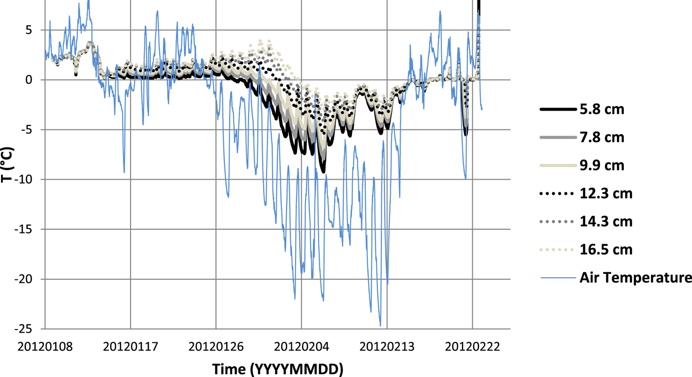
Fig. 3. A temperature record from 8 January 2012 to 22 February 2012 of six data loggers at the depths of 5.8, 7.8, 9.9, 12.3, 14.3 and 16.5 cm below the water level of the pond Dolní Tušimy. Included is the reference air temperature.
A similar experiment was performed in ice over lake Baikal (Aslamov and others, Reference Aslamov2014).
3.2 Ice sampling and data transfer
On 22 February 2012, the volume of ice containing the frozen-in thermochrons was cut out using a handsaw and photographs were taken for the ice structure investigation immediately after the sample retrieval. Photographs were analyzed for bubble concentration, shape differences of bubbles and their size distribution. Data recorded from the seven thermochrons were transmitted using the Blue dot receptor, 1-Wire adapter and the OneWireViewer. Data included temperature in degrees Celsius and date. The deepest logger, located at 19.0 cm depth, did not work properly and could not be used for this study.
3.3 Data processing
Growth rates of ice were estimated from the temperature record of two adjacent sensors (e.g. from sensors at the depths of 5.8 and 7.8 cm). We focused on time since the upper sensor just became a part of the ice cover that continued growing downward until it reached the lower sensor. The first step was to estimate the moment when the upper sensor became part of the ice, and then find out the time when the water was turning into the ice around the lower sensor. This way we obtained the time interval required for the ice to grow from one sensor to next one below. These times were read from the data loggers when the ice temperature reached the freezing point (0°C). We plotted a graph of temperature data (against time) recorded by the lower sensor (in liquid water at the beginning) during this time interval (from the freezing time of upper sensor to the freezing time of lower sensor).
We divided the temperature data according to the rate of temperature decrease, into two parts – an interval of faster decrease of temperature and an interval of slower decrease of temperature. For both intervals, we estimated the value of growth rates by linear interpolation. Separately for each part, we used a linear regression fit (temperature dependence on time) with resulting equation, where we assumed T(t) = 0. Solving this, we obtained an estimated time when the lower sensor would get into the ice, assuming a constant temperature gradient. In this way, we obtained time difference between two sensors recording T(t) = 0°C. The time difference and the depth difference between two sensors were used to determine the growth rate of the ice for the specific period in (μm s−1).
Cooling rates (°C s−1) were calculated as the difference between the maximum and minimum temperature values recorded by the lower sensor near the ice–water interface for given time periods – the same that were used for the calculation of growth rates.
Differentiating equations for calculating growth/cooling rates was used to get Std dev. For values of the growth and cooling rates. The Std dev. derives as (Brož, Reference Brož1983)
 $$\sigma _{G_{\rm r}} = \sqrt {{\left( {\displaystyle{1 \over t}\; \hbox{d}h} \right)}^2 + {\left( {\displaystyle{{ - h} \over {t^2}}\; \hbox{d}t} \right)}^2} \;, $$
for growth rates, and as
 $$\sigma _{C_{\rm r}} = \sqrt {{\left( {\displaystyle{1 \over t}\hbox{d}T} \right)}^2 + {\left( {\displaystyle{{ - T} \over {t^2}}\; \hbox{d}t} \right)}^2}, $$
for cooling rates. Where t is the time, h is the depth, T is the temperature and dh, dt, dT are the Std dev.
Instrument error of the temperature loggers (±0.03°C) was added and subtracted from the first and last temperature values where rates need to be estimated. A system of three linear equations allowed for obtaining errors of modeled time. The deviation error of the depth estimation was set as a half of vertical physical thickness of the thermochron parallel to its cylindrical axis (±0.3 cm). These were used for the final estimate of growth rates (μm s−1) and cooling rates (°C s−1).
We acknowledge that this pond setting does not represent laboratory condition and deviation from true freezing temperature may occur due to dissolved content in water, supercooling and many other effects. Therefore, we assume that the freezing temperature may fluctuate between 0°C and −0.5°C.
3.4 Modeling of ice thickness
The commonly used method for predicting the thickness of ice is based on variations of the Stefan problem for phase transitions in which the thickness is proportional to the square root of the accumulation of degree-days of freezing (Ashton, Reference Ashton1989, Reference Ashton2011). In this method, the difference between the daily average air temperature and the freezing point of water is multiplied by time (days) since initial ice formation, the square root taken and the result multiplied by a coefficient to obtain the predicted ice thickness (Ashton, Reference Ashton1989). The Stefan solution is based on a simple idea that the heat released by freezing at the bottom of ice is conducted upward through the ice by a constant temperature gradient. Specifically, Stefan solution is based on four postulates: (a) no thermal inertia, (b) no internal heat sources, (c) a known temperature at the top, T s = T s(t) and (d) no heat flux from the water (Leppäranta, Reference Leppäranta1993).
This method works well for thicknesses of ice over ~10 cm. For thicknesses <~10 cm, the method overestimates the ice thickness. For specific cases, the use of the traditional method can give incorrect results (Ashton, Reference Ashton1989). The main problem with Stefan solution is the poor knowledge about the top boundary condition. Usually the temperature of the top surface of ice is estimated from the air temperature, which is difficult to do when the ice is thin or when there is a snow cover on the ice. In addition, neglecting the heat flux from the water may lead to unrealistic estimates. This method assumes that the thermodynamic properties of ice are constant (Leppäranta, Reference Leppäranta1993) which may not be the case.
Stefan solution is obtained by using a standard Fourier law for heat conduction expressing the heat flux through the ice in the form
 $$Q_{\rm i} = \; \displaystyle{{ - k\; (T_{\rm m} - T_{\rm s})} \over h},$$
where Q i is the heat flux through the ice, k is the thermal conductivity of the ice, T m is the temperature at the ice–water interface (0°C), T s is the temperature of the top surface (Ashton, Reference Ashton1989) and h is the thickness. T s is taken as the air temperature (T a), although it is not generally true due to boundary layer effects (Ashton, Reference Ashton2011).
At the bottom surface, the heat flux is balanced by the latent heat of fusion of newly formed ice. The rate of the production of the ice at the bottom surface is
 $$\rho L\displaystyle{{\hbox{d}h} \over {\hbox{d}t}} = Q_{\rm i},$$
where ρ is the density of ice, L is the heat of fusion and t is the time (Ashton, Reference Ashton1989, Reference Ashton2011). Combining (4) and (5) and integrating, we get an expression for the ice thickness, h, after time t is then
 $$h = \left( {\displaystyle{{2k} \over {\rho L}}} \right)^{1/2}\lsqb {\lpar {T_{\rm m} - T_{\rm s}} \rpar t} \rsqb ^{1/2}.$$
In practice, data show that an empirical coefficient, α, usually in the range 0.5–0.8, must be applied to the right-hand side to give more realistic estimates (Ashton, Reference Ashton1989). However, the coefficient α includes incorrect assumptions. For example: T s = T a, neglect of the insulating effect of a snow layer and the flux of heat from the water to the undersurface is zero (Ashton, Reference Ashton2011).
Ashton (Reference Ashton1989) added to the Stefan solution the effect of the thermal resistance between the top of the ice surface and the bulk temperature of the air. It provides an analytical result which is applicable for both thin and thick ice.
In addition to Eqns (4) and (5) above, the flux of heat Q ia from the ice surface to the air above can be expressed in the form of a bulk heat transfer coefficient H ia applied to the difference between the top surface temperature of the ice and the air temperature above the ice, resulting in
 $$Q_{{\rm ia}} = \; H_{{\rm ia}}(T_{\rm s} - T_{\rm a}),$$
which is Newton's law of cooling.
If the heat flux through the ice equals the heat flux from the surface of the ice to the air above, then T s may be eliminated using Eqns (4), (5) and (7). It results in
 $$\displaystyle{{\hbox{d}h} \over {\hbox{d}t}} = \; \displaystyle{1 \over {\rho L}}\; \displaystyle{{T_{\rm m} - \; T_{\rm a}} \over {\lpar {(h/k) + \; (1/H_{{\rm ia}})} \rpar }}.$$
This may be integrated (with the boundary condition that h = 0 when t = 0) and results in
 $$h = \left[ {\displaystyle{{2k} \over {\rho L}}\; \lpar {T_{\rm m} - \; T_{\rm a}} \rpar + {\left( {\displaystyle{k \over {H_{{\rm ia}}}}} \right)}^2} \right]^{1/2} - \; \displaystyle{k \over {H_{{\rm ia}}}}$$
(Ashton, Reference Ashton1989).
To apply (9) in practice, the bulk heat transfer coefficient must be determined. One way of doing this is to apply detailed energy budget methods to the top surface of the ice, calculate the net transfer Q ia, determine T s and then determine H ia by dividing with the temperature difference T s − T a (Ashton, Reference Ashton1989). The accurate value of the bulk transfer coefficient (H ia) depends on the various components of the energy budget, but it usually falls between 10 and 30 W m−2 °C−1. Higher values are associated with windy conditions and lower values with still air conditions, but, with other information unavailable, a value of 20 W m−2 °C−1 fits data on ice growth well (Ashton, Reference Ashton1986, Reference Ashton1989, Reference Ashton2011).
For modeling the thickness of the ice cover over the pond DT, we used two methods. The first one was based on simplified solution of the Stefan problem (Eqn (6)). The coefficient α was set as 1, 0.7 and 0.5. For the second method, we used Ashton's solution (Eqn (9)) with the bulk heat transfer coefficient (H ia) 10 and 20 W m−2 K−1. When we calculated the daily increment of ice, we used the average temperature of the air. Assuming the temperature profile within the ice was linear, we estimated, based on our temperature data, mean temperature of the ice surface. We used this estimate instead of the air temperature when solving Eqn (6) for chosen periods of time.
These two methods of calculating thickness of ice do not include an effect of the heat flux from water to ice (Q wi), although neglecting it may sometimes lead to unrealistic results. This heat flux may melt ice, or to prevent melting, it must be conducted away through the ice (Leppäranta, Reference Leppäranta1993). If the temperature gradient at the ice–water interface and the conductivity are known, the heat flux from the water to the ice can be estimated using the gradient method (Malm and others, Reference Malm1997a, Reference Malmb; Kirillin and others, Reference Kirillin2012):
 $$Q_{{\rm wi}\; = \; k_{\rm w}}\displaystyle{{\partial T} \over {\partial \hbox{h}}},$$
where k w is thermal conductivity of water, which depends on the flow regime (Kirillin and others, Reference Kirillin2012) and h is a distance from the ice–water interface. The heat flux from water to the ice is formed in a multilayer system formed by a laminar microzone at the contact with the ice cover, a transition zone and a turbulent water column (Aslamov and others, Reference Aslamov2014).
4. RESULTS
The first ice that was formed over the pond DT occurred around 14 January 2012. All sensors read temperature near 0°C and the water column was well mixed. The formation of permanent ice cover of thickness exceeding 5.8 cm did not begin until 27 January 2012. During the data analysis of loggers, we focused on the period from 29 January 2012 to 3 February 2012.
The temperature data spanning these 6 d are shown in Figure 4a. During this time, the temperature of all six sensors dropped below the freezing point (0°C) and they successively became part of the ice as the ice thickened. Figure 4a also clearly shows the air temperature variations which are a result of the diurnal cycle (Kletetschka and others, Reference Kletetschka, Fischer, Mls and Dedecek2013).
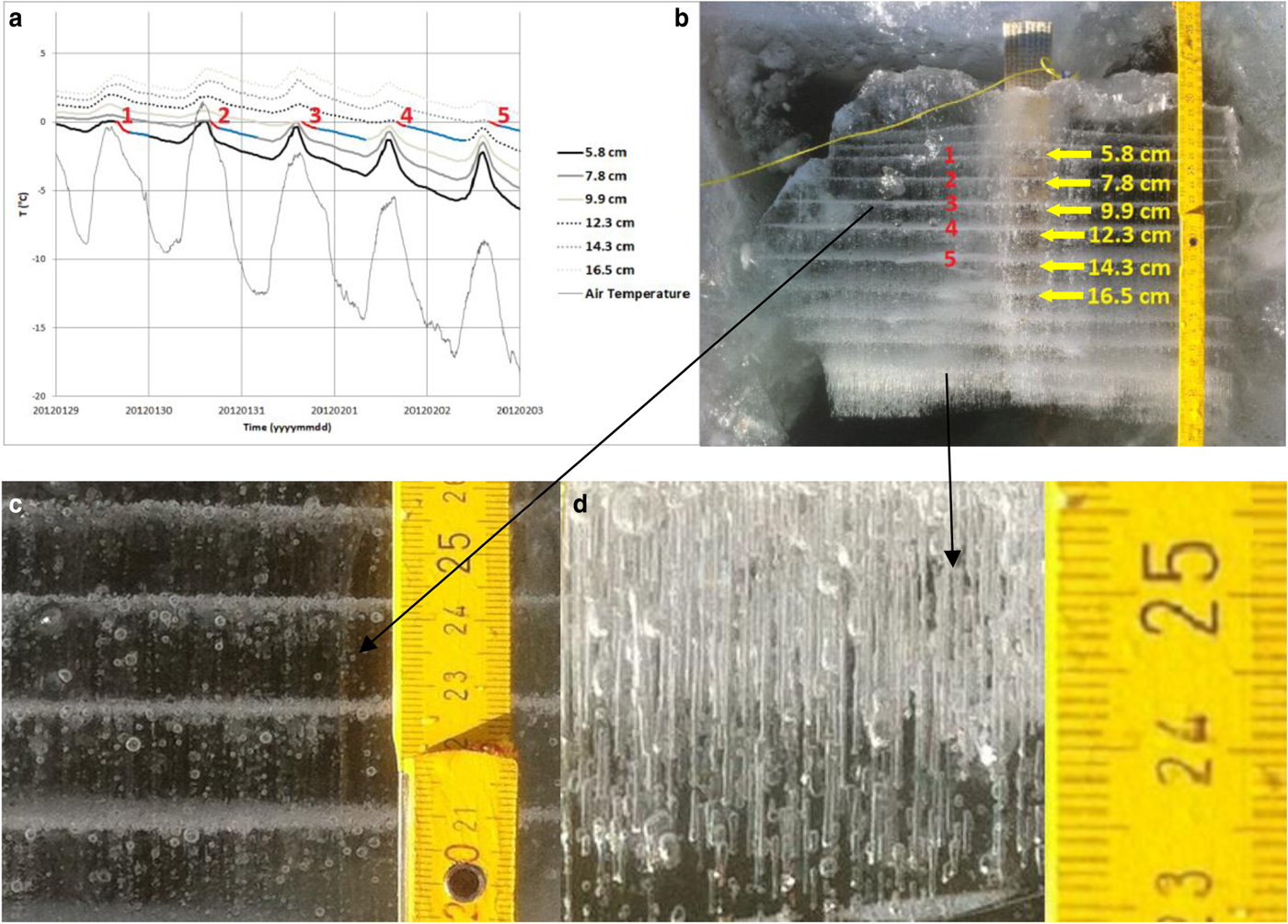
Fig. 4. Relationship between temperature records and bubble layer texture. (a) Comparison of the temperature record from six temperature data loggers. Numbers 1, 2, 3, 4, 5 indicate respective layers of bubbles in (b). Red parts of the graph represent time intervals when these layers were formed. Red and blue parts were used for growing and cooling rate calculations. (b) Photograph of the ice sample from the pond Dolní Tušimy. Arrow points to the individual sensors at a depth of 5.8, 7.8, 9.9, 12.3, 14.3 and 16.5 cm. (c) Detail of the bubble layers separated by ice with fewer bubbles. Note the presence of rounded gas bubbles. (d) Detail of the lower most part of the ice where we identified the presence of cylindrical gas bubbles.
The ice grew, captured all our temperature sensors and generated a layered texture. Figure 4b shows this layered texture which was imaged after the ice retrieval. The multiple horizontal layers of gas bubbles were clearly distinct. Throughout the thickness of the ice ~13 layers of bubbles were observed. Vertical thickness of each of the bubble layers was <1 cm. They were separated by ~2 cm-thick layers of ice with low concentration of gas bubbles distributed randomly in space. The shape of the bubbles in the sample of ice from the pond DT was mostly rounded (Fig. 4c). The size of bubbles forming layers was smaller (usually <1 mm in diameter) than that of bubbles outside these layers which were ~1–2 mm in diameter.
Additional thickening (growth) of ice depends mainly on the low temperature of overlying air (top surface of ice) that removes heat from the ice–water interface (Ashton, Reference Ashton1989, Reference Ashton2011). The thermal exchange between water and atmosphere leads mainly to growth or thawing of the ice cover. Heat loss from water through the ice cover results mostly in thickening of ice and not in water cooling (Bengtsson and Svensson, Reference Bengtsson and Svensson1996). Table 1 shows an alternation of high and lower growth rates of ice as well as cooling rates during the period of our interest (29 January–3 February). Mean temperatures of the ice surface and mean temperatures at the depths of 5.8 and 16.5 cm from the top surface of the ice are also listed in Table 1. Although the mean temperature of the ice surface kept decreasing with time, the rates of both growth and cooling were increasing and decreasing, respectively.
Table 1. Alternation of the maximum growth and cooling rates of ice and growth and cooling rates of ice leading to the formation of the ice with low concentration of gas bubbles

T air, mean temperature of the air; T surface, mean temperature of the top surface of the ice; T 5.8, mean temperature at the depth of 5.8 cm from the top surface of the ice; T 16.5, mean temperature at the depth of 16.5 cm from the top surface of the ice.
Despite decreasing temperature of the ice surface, the growth rate of ice decreased with time. This was due to the increasing thickness of the ice which provided thermal insulation and due to increasing values of the heat flux from warmer water. The lower growth rates with thicker ice present is a result of the insulating properties of the bubbles (Haynes and Lide, Reference Haynes and Lide2011). Mean heat fluxes from the water to the ice are shown in Table 2. For their calculation, we used Eqn (10) with k w = 0.6 W m−2 °С−1 (molecular water conductivity). For calculation of temperature gradients, we used depths from the beginning of each period although we know it is not correct as the ice was growing and the distance from the ice–water interface was changing.
Table 2. Increasing values of cooling rates related to the temperature gradients below the ice ∂T/∂h(wi), and to mean heat fluxes from the water to the ice Q wi.
∂T/∂h(w) represents temperature gradient in the water and Q w heat flux in the water.
Values of cooling rates (°C s−1) in the vicinity of ice–water interface (see Tables 1 and 2) increased with time. They were related to temperature gradients and heat fluxes within the ice and from the water to the ice. The greater temperature gradient, the greater heat flux and faster cooling. Temperature gradients between ice–water interface (0°C) and the first sensor down in the water are listed in Table 2 as well as heat fluxes from the water to the ice. We considered it important to also include temperature gradients and corresponding minimal (k w = 0.6 W m−2 °С−1) heat fluxes Q w between the first and the second sensors in the water below the ice (Table 2). These explained the differences between cooling rates with similar heat fluxes Q wi.
Figure 5 shows a comparison of calculated model results for two methods of predicting the thickness of the ice with the observed values of thickness. During days from 28 January to 12 February, the daily mean temperature of the air was below the freezing point of water (see Table 3), and so the ice was growing. In the following days, the daily mean temperature of the air was temporarily above freezing and the ice could potentially get thinner. Ice thinning was not accounted for in the model (Fig. 5). Both calculated methods overestimated the ice thickness. For thicker ice (more than ~10 cm), the overestimation was greater. The estimate closest to the observation was obtained by the bulk heat transfer coefficient (H ia) with a value of 10 W m−2 °C−1.

Table 3. Observed depths of ice growing over the pond Dolní Tušimy on 14 January 2012–22 February 2012 with the mean daily air temperature and growth rates of ice
For predicting the thickness of ice based on Stefan solution, the temperature of the ice surface is taken as the air temperature, although this is not generally true (Ashton, Reference Ashton2011). We estimated the temperature of the surface of the ice and used it instead of the air temperature for calculation of the increment of ice during periods of high/low growth/cooling rates. Due to our data and values of growth rates, we were able to get an increase in ice thickness for these periods of time and compared it with the thicknesses of ice calculated using Eqn (6) modified by an additional heat flux of the water to the ice (see Table 4). The empirical coefficient α was set as 0.5, 0.7 and 1. Thicknesses of the ice were also overestimated.
Table 4. Comparison of thicknesses of the ice estimated based on our data (marked with *) with calculated thicknesses using traditional method
5. DISCUSSION
The occurrence of gas bubbles in pond ice relates mostly to the gas content in the water and to the growth rate of ice (Yoshimura and others, Reference Yoshimura, Inada and Koyama2008; Inada and others, Reference Inada, Hatakeyama and Takemura2009). As concentration of bubbles within the ice increased with an increase of ice growth rate (Yoshimura and others, Reference Yoshimura, Inada and Koyama2008; Madrazo and others, Reference Madrazo, Tsuchiya, Sawano and Koyanagi2009), the layers of bubbles indicated higher growth rate of the ice. When comparing the temperature record (Fig. 4a) and the photo of the ice sample shown in Figure 4b, we could estimate the approximate time when individual layers of bubbles had formed. Five layers of bubbles were identified with successive numbers 1, 2, 3, 4 and 5, both on the photograph and on the temperature record. Red parts of the graph in Figure 4a indicate the time intervals when freezing of pond water progressed fast and formed layers of bubbles.
Most studies (Bari and Hallett, Reference Bari and Hallett1974; Yoshimura and others, Reference Yoshimura, Inada and Koyama2008; Madrazo and others, Reference Madrazo, Tsuchiya, Sawano and Koyanagi2009) reported that when bubbles are incorporated into the ice crystal, they are typically egg-shaped or cylindrical. The egg-shaped bubbles become dominant with increasing growth rates and the cylindrical bubbles occur at lower growth rates (Bari and Hallett, Reference Bari and Hallett1974; Madrazo and others, Reference Madrazo, Tsuchiya, Sawano and Koyanagi2009). The bubbles of cylindrical shape in our ice occurred only at the bottom of the ice sample (Fig. 4d). It might be due to lower growth rate, as the layer of ice above provided an increasing thermal insulation with increasing ice thickness.
Bari and Hallett (Reference Bari and Hallett1974) stated that the ice growth rate, which gave egg-shaped bubbles, was ~25 µm s−1. Growth rates of the reported ice, when formed at <25 µm s−1, gave cylindrical bubbles, which ceased entirely at ~3 µm s−1, to give completely clear ice. The growth rates for the pond DT are in Table 1, maximum values varied from 0.58 to 0.92 µm s−1. These growth rates caused the formation of layers of gas bubbles within the ice. Lower growth rates led to the formation of the ice with low concentration of gas bubbles (Table 1).
We note that the growth rates of ice associated with the formation of bubbles were lower for the pond DT than those obtained experimentally by Bari and Hallett (Reference Bari and Hallett1974). This discrepancy has been seen in lakes (see Gow and Langston (Reference Gow and Langston1977)), but this is the first report in ponds, and it is likely related to the impurity content of the pond DT. Although the water in the pond appeared clear (which is common during the winter), we believe that the impurity content is greater than that of the distilled water used by Bari and Hallett in their experiments. The impurities serve as a center of nucleation of gas bubbles.
According to our data, we can see (in Table 1) that lower temperatures of the air did not mean higher values of growth rates. So there are additional factors (such as solar radiation, wind-speed, humidity, precipitation, etc.) influencing thickening of ice (Ashton, Reference Ashton2011; Ajne, Reference Ajne2013) much more than the air temperature. While the mean temperature of the ice surface kept decreasing with time, the rates of both growth and cooling were increasing and decreasing, respectively. We interpret this observation as an effect of the heat flux from the water to the ice, and of gas concentration changes in the water.
There was no snow cover over the ice, so a sufficient amount of solar radiation could penetrate through the ice and heated the water below. The greater the temperature gradient in the vicinity of the ice–water interface, the greater heat flux from the water to the underside of the ice.
When the ice volume increased, it displaced most of the dissolved gas into the water below. As the pond is shallow, most of the water column was heated up to 4°C (see Fig. 4a). Increasing temperature of underlying layers of water might cause gas release (due to decreasing water solubility) which was related to gas bubble formation. Bubbles eventually appeared in the vicinity of the ice–water interface where they served as an insulator and they protected the ice from the heat flux from the water. Ice growth could progress quickly, and some gas bubbles became part of newly formed ice. With no (or less) bubbles in the vicinity of the ice–water interface, there was the heat flux from the water which reduced ice growth at the bottom.
Growth of the ice from one sensor to another (distance ~2.0–2.4 cm) lasted ~9–18 h. We can read it from our temperature data as adjacent data loggers recorded successively freezing temperature (0°C) and so we set time intervals for our calculation (Tables 1–3). Time between these intervals usually lasted ~6–16 h. During this time, temperature recorded by the sensor just frozen in ice was still near freezing point or even slightly above it. We neglect any further increase in ice thickness at that time.
Model calculations resulted in growth rate overestimation. This is likely due to neglecting the heat flux from the water to the ice and the effect of gas bubbles at the ice–water interface. As our data show (in Fig. 4a), the layer of water under stable ice cover may be heated due to solar radiation (assumed a clear sky and snow absence) which can cause significant heat flux to the underside of the ice. This might cause deviation from the modeled thicknesses. Some discrepancy could also arise from the fact that the air temperatures, used for calculations, were not measured at the place of the pond but 1.5 km away.
Allison (Reference Allison1979) stated in his work on Antarctic sea ice growth that using the classical relationship between the thickness of ice and air temperature, Stefan's law, greatly overestimates the growth rate because of neglecting the role of heat flux from the ocean to the ice at the lower boundary. Allison (Reference Allison1979) also considered it important that only long-term intervals should be used to minimize the effect of lag between the surface temperature and the ice growth rate. These factors could have contributed to uncertainties in our experiments and modeling.
6. CONCLUSIONS
We identified the specific environmental record from a distinct horizontal accumulation of bubbles in the ice in the pond DT in Mokrovraty, Czech Republic. These accumulations of bubbles were separated by ~2 cm layers of ice with low concentrations of gas bubbles that were arranged randomly in space. The shape of these bubbles was mostly rounded. Bubbles of cylindrical shape, however, occurred near the bottom of the ice sample. They indicated lower growth rates of this ice, as the layer of the ice above provided an increased thermal insulation after the thickness of the ice increased significantly. The size of the bubbles within layers of accumulation was smaller than that of the bubbles outside these layers due to the faster mode of their formation.
Our data confirm the relation between growth rates of ice and the occurrence of bubbles in ice. If the water/ice phase change occurs rapidly and the growth rate of ice is high, the concentration of bubbles incorporated into ice crystals is high and bubbles are small. The comparison with similar work done showed an important distinction relevant for the environmental record. The ice growth rates associated with the formation of bubbles in natural ice over the pond were lower (0.58–0.92 µm s−1) than those obtained experimentally (Bari and Hallett, Reference Bari and Hallett1974). This discrepancy was caused by obvious impurity content of the pond and emphasizes the difference between the experimental and natural behavior of ice.
We showed that growth rates and cooling rates of natural ice can be determined from the temperature data recorded by autonomous data loggers. Autonomous data loggers revealed that periods of high and low growth rate alternated. This was an effect of the heat flux from the water to the ice, which was modified by the concentration of gas bubbles located in the vicinity of the ice–water interface. The growth rates of ice decreased toward greater depths (with time) as the increasing thickness of the ice provided thermal insulation and heat flux from warmer water increased. Values of cooling rates measured in the vicinity of the ice–water interface increased with time and they were affected by the water to ice flux.
Using of traditional computational methods (Ashton, Reference Ashton1986, Reference Ashton1989; Leppäranta, Reference Leppäranta1993) for the determination of ice thickness overestimated the pond results and showed their limitations when applied to the growth of ice under natural conditions. We conclude that the heat flux from the water to the ice, the effect of gas bubbles in the vicinity of the ice–water interface and using variable thermal properties of the ice with depth and time would improve this model (Allison, Reference Allison1979; Ashton, Reference Ashton2011).
This work reveals that during the fast ice growth periods, the ice structure is modified by the occurrence of gas bubbles that may compromise the structural properties of ice. Additionally, our method enables an estimation of the approximate time when the specific ice was formed, and this unique dataset will constrain future modeling of natural ice over ponds/lakes.
ACKNOWLEDGEMENTS
We thank Marek Hora for his help in the field and Matthew Morgan Markley for reading the manuscript and helpful comments. We thank Tony Gow, Allen Lunsford and Peter Wasilewski for helpful discussions. This work was supported by grants GACR 17-05935S, RVO 67985831. The work was also supported by Ministry of Education, Youth and Sports of the Czech Republic (LK21303). Data related to this research are available at: https://docs.google.com/a/natur.cuni.cz/viewer?a=v&pid=sites&srcid=bmF0dXIuY3VuaS5jenxldGdlbnxneDozZTY5MTRmZGQ1MjZmNzJm.


 Open access