


1. Introduction
Recent high spatial-resolution geodetic glacier mass-balance observations over the Himalaya and Karakoram (Vijay and Braun, Reference Vijay and Braun2016; Brun and others, Reference Brun, Berthier, Wagnon, Kaab and Treichler2017; Shean and others, Reference Shean2020), as well as other glacierised regions (McNabb and others, Reference McNabb2021) have provided important insights into glacier response to climate change. A limitation of such geodetic datasets is that only the decadal-scale elevation changes can be resolved accurately given the typical uncertainties associated with digital elevation models. The decadal-scale mass change is influenced by both glacier dynamical effects and the climate forcing. In contrast, the annual-scale variability directly reflects the meteorological forcing on the glacier, since the glacier geometry does not change appreciably over such short time scales (Banerjee, Reference Banerjee2017). It is also important from a water-resources perspective because of its control over the variability of runoff of glacierised catchments (e.g. Fleming and Clarke, Reference Fleming and Clarke2005; Banerjee, Reference Banerjee2022).
Annual to seasonal glacier surface mass balance can be obtained by direct field measurements at ablation stakes drilled into the ice and at snow pits. This ‘glaciological’ method is considered to be one of the most accurate methods for assessing glacier mass balance (Kaser and others, Reference Kaser, Fountain and Jansson2003). However, such measurements are available only for a small fraction of global glaciers. This data gap may be addressed using indirect estimates of the annual mass balance via remotely-sensed proxies (e.g. Racoviteanu and others, Reference Racoviteanu, Williams and Barry2008; Rabatel and others, Reference Rabatel2017), or through numerical modelling (e.g. Kumar and others, Reference Kumar2019). Most remote-sensing-based methods rely on determining the end-of-summer snow-line altitude (SLA) over the glacier surface (e.g. Kulkarni, Reference Kulkarni1992; Rabatel and others, Reference Rabatel, Dedieu and Vincent2005). The estimated SLA is taken to be a proxy of the equilibrium-line altitude (ELA). A strong correlation between ELA and annual mass balance then allows a reconstruction of the annual-scale mass balance simply by applying a linear transformation to the observed time series of SLA. To find the optimal linear transformation, long-term glaciological mass-balance records are used (e.g. Kulkarni, Reference Kulkarni1992; Rabatel and others, Reference Rabatel, Dedieu and Vincent2005). However, there are certain intrinsic limitations associated with the determination of SLA (Rabatel and others, Reference Rabatel2017). For example, the snowline does not strictly follow any elevation contour, and the identification of SLA from terrestrial (e.g. Barandun and others, Reference Barandun2018) or satellite (e.g. Rabatel and others, Reference Rabatel, Dedieu and Vincent2005) images is often difficult, requiring manual interpretation of the reflectance contrast. Another glacier-specific proxy for the annual balance is the minimum value of the albedo over the glacier or a suitable part of it (e.g. Brun and others, Reference Brun2015; Davaze and others, Reference Davaze2018). This is relatively straightforward to compute. However, the data gaps due to the finite repeat cycle of the satellite used and/or the presence of cloud cover compromise the accuracy of all the above snowcover-based proxies (Rabatel and others, Reference Rabatel2017).
Perhaps the most critical limitation of the above remote-sensing-based methods is the need for long-term glaciological field observations for calibration. This prevents any reconstruction of annual mass balance for most of the glaciers in data-sparse regions like the Himalaya and Karakoram. Additional complications arise in regional studies when a proxy-based method calibrated for a particular glacier is generalised over the whole region under some strong assumptions. For example, a linear transformation calibrated for a single glacier may be applied to all the glaciers in a region (e.g. Tawde and others, Reference Tawde, Kulkarni and Bala2017), even though it is expected to vary between glaciers. Or, a parameter like the mass-balance gradient at the ELA may be assumed to remain constant across the whole region and between years (e.g. Rabatel and others, Reference Rabatel, Dedieu and Vincent2005). A strong variability of the mass-balance gradient between glaciers, between different branches of a single glacier and between years has been reported (Rabatel and others, Reference Rabatel, Dedieu and Vincent2005; Mandal and others, Reference Mandal2020; Wagnon and others, Reference Wagnon2021). For certain proxies like minimum albedo (Brun and others, Reference Brun2015) a transferable model is not yet known.
Given the above limitations of the existing remote-sensing methods in obtaining glacier-wide mass-balance estimates at an annual scale, here we aim to develop a method that (1) uses only remotely-sensed geodetic mass balance for calibration, (2) does not require any field data and (3) can be applied to any available set of linear proxies of annual mass balance. Such a method would potentially allow a reconstruction of the annual mass balance on any glacier with accurate geodetic mass-balance data, as long as a set of suitable proxies can be identified and accessed. In this paper, we propose such a multi-proxy and purely remote-sensing-based method. Two easy-to-compute proxies for the annual mass balance that are based on the normalised difference snow index (NDSI) (Hall and Riggs, Reference Hall and Riggs2011) are introduced. The reconstruction method is tested on Chhota Shigri Glacier in the Indian Himalaya, and Saint-Sorlin and Argentière glaciers in the French Alps. These glaciers were chosen based on the availability of glaciological mass-balance data, so that the reconstructed estimates could be validated. The two NDSI-based proxies proposed here, and previously reported estimates of SLA and minimum albedo were used for the multiproxy mass-balance reconstructions at an annual scale.
2. Study area and datasets
We considered three valley glaciers (Fig. 1) for the present study: Chhota Shigri Glacier in the Indian Himalaya (32.27°N, 77.52°E; RGI60-14.15990), Argentière Glacier in the French Alps (45.95°N, 6.98°E; RGI60-11.03638) and Saint-Sorlin Glacier in the French Alps (45.17°N, 6.15°E; RGI60-11.03674). Chhota Shigri and Argentière glaciers are similar in size (15.6 and 13.8 km2, respectively (RGI, 2017)). These two glaciers are mostly clean, with some supraglacial debris over the lower ablation zone. Saint-Sorlin Glacier is relatively small (2.7 km2 (RGI, 2017)) and debris free. All the three studied glaciers receive snowfall mostly over the boreal winter months.
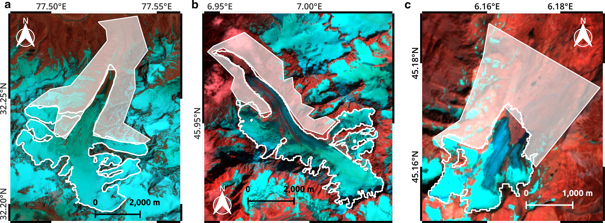
Fig. 1. Sentinel-2 satellite images from July–August 2021 showing the three studied glaciers : (a) Chhota Shigri, (b) Argentière and (c) Saint-Sorlin glaciers. The top-of-atmosphere, false-colour composites were prepared using bands 12, 4 and 2. The glacier outlines (RGI, 2017) are in white. The off-glacier areas shown with stippled white polygons were used to compute the mean daily NDSI (see text for details).
An existing 17-year long (2003–2019) continuous glaciological mass-balance time series on Chhota Shigri Glacier (Mandal and others, Reference Mandal2020) was utilised in this study (Supplementary Table S1). Here the term ‘annual’ refers to the hydrological year that starts on 1 October of a given calendar year, and ends on 30 September of the next calendar year (Mandal and others, Reference Mandal2020). Continuous glaciological mass-balance records for the two French glaciers during 2000–2019 were obtained from www.wgms.ch (Supplementary Tables S3, S5). For these glaciers, several geodetic mass-balance estimates have been reported in the literature spanning different periods over the last two decades (Supplementary Tables S2, S4, S6).
Annual SLA estimates spanning most of the study period were available for all the studied glaciers (Chandrasekharan and others, Reference Chandrasekharan, Ramsankaran, Pandit and Rabatel2018; Davaze and others, Reference Davaze, Rabatel, Dufour, Hugonnet and Arnaud2020). Annual estimates of the glacier-wide minimum albedo over more than a decade were also reported previously (Brun and others, Reference Brun2015; Davaze and others, Reference Davaze2018). In addition, we estimated two NDSI-based proxies for these glaciers over the period 2000–2020 using a Moderate Resolution Imaging Spectroradiometer (MODIS) product (Hall and Riggs, Reference Hall and Riggs2016). The time series of the four proxies used in the present study are provided in Supplementary Tables S1, S3 and S5.
3. Methods
We used four different remotely-sensed proxies to obtain the corresponding estimates of the annual mass balance via a set of four linear transformations. The linear transformations were calibrated separately using the available decadal-scale geodetic mass-balance data (b geo). The reconstructed mass-balance records (b rec) were validated using the available glaciological measurements of annual mass balance (b gla).
3.1 Proxies for annual mass balance
3.1.1. Snow-line altitude (SLA)
Images from LANDSAT, Indian Remote Sensing Satellite series and TerraSAR archives were previously used to delineate SLA on Chhota Shigri Glacier over the past two decades (Chandrasekharan and others, Reference Chandrasekharan, Ramsankaran, Pandit and Rabatel2018). We utilised an updated version of the SLA dataset over the period 2000–2019 (Supplementary Table S1) as one of the proxies here. For the French glaciers, SLA time series between 2000 and 2016 were obtained using images from satellites like LANDSAT, ASTER and Sentinel-2 (Davaze and others, Reference Davaze, Rabatel, Dufour, Hugonnet and Arnaud2020). The time series of SLA and glaciological mass balance had a correlation coefficient r = −0.74 and −0.77 (p < 0.001) on Chhota Shigri and Argentière glaciers, while the correlation was weak and insignificant for Saint-Sorlin Glacier (Fig. 3a, Supplementary Figs S1a, S2a).
3.1.2. Albedo
Previously reported MODIS-derived annual minimum albedo time series over a selected part of the glacier surface, spanning about 15 years, were utilised here for Chhota Shigri Glacier (Brun and others, Reference Brun2015) and the two French glaciers (Davaze and others, Reference Davaze2018). Hereinafter, we refer to this proxy as minimum albedo for brevity. On all the three glaciers, the minimum albedo was well correlated with the corresponding glaciological mass balance with r in the range 0.81–0.90 (p < 0.001) (Fig. 3b, Supplementary Figs S1b, S2b). Note that the existing method (Brun and others, Reference Brun2015) to convert the minimum albedo data to annual mass-balance estimates cannot be applied to a glacier without long-term glaciological mass-balance records.
3.1.3. Normalised difference snow index
NDSI is the ratio of the difference to the sum of the visible and near-infrared reflectances (Hall and Riggs, Reference Hall and Riggs2011). It ranges between −1 and +1, with a high NDSI indicating the presence of snowcover (Riggs and Hall, Reference Riggs and Hall2016). We tested if any statistics of mean daily NDSI over the part of the valley surrounding the ablation zone of the glacier studied during the summer months can serve as a reliable proxy for the annual mass balance. The NDSI-based proxies were defined over the off-glacier area surrounding the ablation zone (Fig. 1). Hereinafter, we refer to this chosen area as the periglacial area for convenience. The periglacial area was considered here as it was likely to have a relatively larger interannual NDSI variability than on the glacierised area due to the presence of perennial ice and/or snow cover over the glacier surface. For example, the range of daily NDSI on Chhota Shigri Glacier and the corresponding periglacial area were −0.01 to 0.93, and −0.21 to 0.90, respectively. The chosen area extended laterally up to the valley ridges and a suitable distance downvalley, so that it had a size comparable to that of the glacier. We did not optimise the chosen periglacial area as the same exercise is not feasible on glaciers without glaciological mass-balance data. However, we repeated the calculations for a couple of different choices of the periglacial area to confirm that the precise definition of the zone was not important.
The raw NDSI values of the MOD10A1 V6 Snow Cover Daily Global 500 m product from MODIS (Hall and Riggs, Reference Hall and Riggs2016) for the period 2000–2020 were accessed with Google-Earth Engine, and subsequently analysed using the R software (R version 3.6.3, R Core Team 2020). We tested two different NDSI proxies: (1) the mean of the raw NDSI, (2) the mean NDSI after removing the pixels with cloud cover using the no-data flags of the associated snow-cover product (Riggs and Hall, Reference Riggs and Hall2016). The former choice of using the raw NDSI values was motivated by a reported dependence of the glacier mass balance on both snowfall and cloud cover (e.g. Kumar and others, Reference Kumar2019). To identify appropriate statistics of the monthly distribution of the mean NDSI, we computed 0, 10, …, 100 percentile values of the mean daily NDSI for each of the 12 months from 2000 to 2020. The correlation coefficients (r) between the time series of each of these percentile values and the available glaciological mass-balance records on Chhota Shigri Glacier suggested that the 10-percentile raw NDSI value (r = 0.87, ~p < 0.01) and the 40-percentile cloud-filtered NDSI values (r = 0.86, ~p < 0.001) for the month of July were two suitable choices (Figs 2a,c). These two proxies are denoted by NDSI1 and NDSI2, respectively, for the rest of the paper. For the two French glaciers, we used the same definitions of NDSI1 and NDSI2.
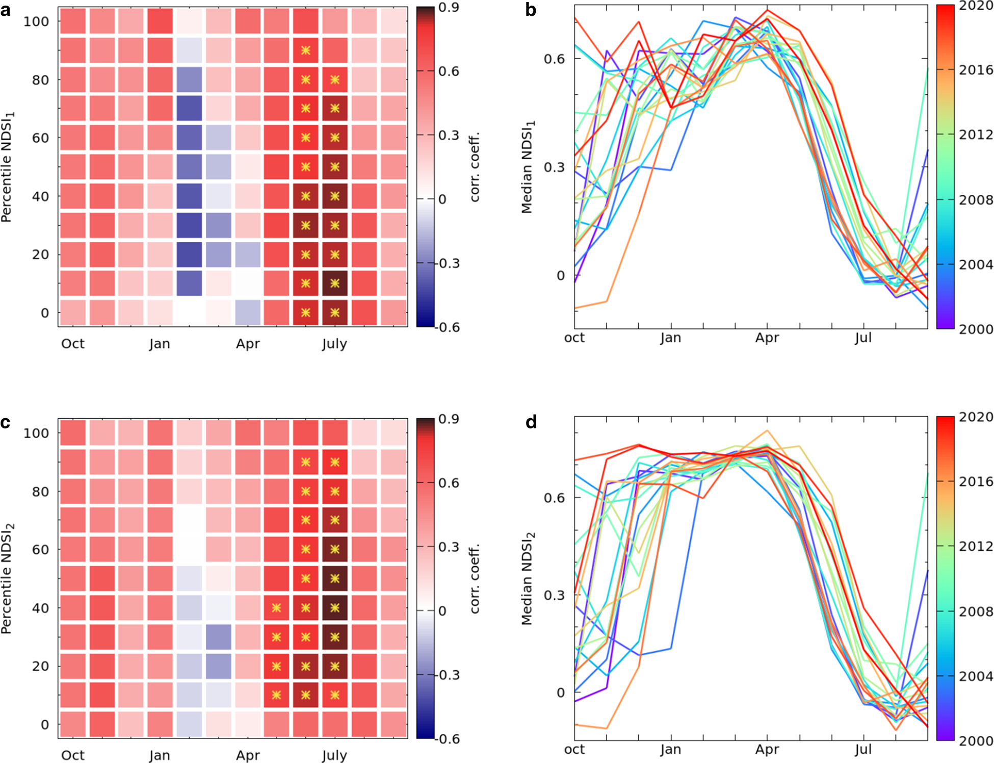
Fig. 2. (a) and (c) Colormaps of correlation coefficients between glaciological mass balance and the percentiles of monthly NDSI1 and NDSI2 averaged over the periglacial area of Chhota Shigri Glacier. The yellow stars denote correlations significant at p < 0.001. (b) and (d) Monthly median of the mean daily NDSI1 and NDSI2 for the period 2000–2020.
The observed relationship between the above proxies and the available glaciological mass-balance records on Chhota Shigri Glacier (Fig. 3) and the two French glaciers (Supplementary Figs S1, S2) confirms the usefulness of the proxies. However, for some of the proxies (e.g. NDSI2), there were signs of saturation for the most negative of the mass-balance years. Such limitations (e.g. nonlinearity/saturation, interference due to cloud cover etc.) associated with remotely-sensed proxies of glacier mass balance are well-known, and have been discussed in detail previously (e.g. Rabatel and others, Reference Rabatel2017).

Fig. 3. (a–d) Comparison between glaciological mass balance and the remotely-sensed proxies on Chhota Shigri Glacier. In all the sub-figures, the number of data points n, the correlation coefficient (r) and its statistical significance (p) are indicated. The corresponding best-fit trend lines are also shown (solid line).
3.2. Calibration of proxies using geodetic mass-balance data
For any suitable proxy, which is linearly correlated with the annual mass balance of a given glacier, the annual balance can be estimated as,

Here b rec and ${\cal P}$ denote the values of the reconstructed annual mass balance and the proxy, respectively, for a given year. The fit parameters of this linear transformation are α (m y.e. a−1) and β. The unit of β depends on the specific choice of ${\cal P}$
 , e.g. it is m w.e. a−1 for dimensionless proxies like minimum albedo or NDSI. It follows that the reconstructed mean mass balance between the years y and y + δy can be obtained as,

Here 〈…〉y,δy denotes the average value between the years y and y + δy. Given N( > =2) available geodetic mass-balance records, the free parameters α and β can be uniquely determined by a straightforward linear regression, which minimises the total squared deviation between the geodetic and the reconstructed mean mass balance, i.e.

Here b geo,j is the j-th geodetic record spanning the years y j to y j + δy j. To minimise the impact of inherent noise in the geodetic data, we used all the available geodetic records, making N as large as possible. Only the geodetic data points that were clear outliers compared to the other geodetic or glaciological records were ignored.
3.3. Multi-proxy reconstruction and its uncertainty
The best-fit linear transformation for each of the proxies was used to obtain four different reconstructions of the annual balance. These four reconstructions were averaged to derive the final multi-proxy estimate of b rec. Note that the above procedure is entirely based on remotely-sensed proxies, which are calibrated using geodetic mass balance without referring to any field data whatsoever. We acknowledge that the different proxies used for a given glacier may not be equally reliable. However, it is not possible to ascertain the relative performance of the proxies without independent estimates, either glaciological or model-based, of annual mass balance. Therefore, we use arithmetic averaging to combine the results from each of the proxies.
A Monte-Carlo method estimated the uncertainties in the reconstructed mass-balance records. We repeated the above fits 500 times for each of the proxies. In each of these runs, an independent random Gaussian noise was added to each of the geodetic and proxy records. The standard deviation of the noise in geodetic data was the median (0.16 m w.e. a−1) of the reported errors in the geodetic measurements on Chhota Shigri glacier, which varied in the range 0.05–0.34 m w.e. a−1 (Supplementary Table S2). For SLA and the other three dimensionless proxies, the standard deviations of the noise were taken to be 80 m and 0.05, respectively. These values were $\sim 20\percnt$ of the range of variability of the respective proxies on Chhota Shigri Glacier over the study period, and were comparable to the previously reported uncertainties in these proxies (Brun and others, Reference Brun2015; Chandrasekharan and others, Reference Chandrasekharan, Ramsankaran, Pandit and Rabatel2018; Davaze and others, Reference Davaze2018, Reference Davaze, Rabatel, Dufour, Hugonnet and Arnaud2020). The standard error computed from the ensemble of reconstructions obtained the 1-σ uncertainty in b rec.
3.4. Validation of the multi-proxy reconstruction
The multi-proxy reconstructions of the annual mass balance of the three studied glaciers were compared with the corresponding glaciological records, by computing the root-mean-squared error (RMSE), bias and correlation coefficient (r) between the time series of b rec and b gla. The reconstructed values were also compared with all the proxy- and modelling-based reconstructions available in the literature for Chhota Shigri Glacier. We also compute the mean biases between the b gla and b geo records, and between available b gla and b geo data on all the three studied glaciers.
While our reconstruction was based solely on geodetic mass balance, the proxies of the annual mass balance were chosen with the help of available glaciological data. Once a proxy is established for a glacier, it may be expected to work for other glaciers having a similar climate and/or morphology. However, the reconstructed interannual mass-balance variations can only be validated for glaciers where other independent proxy- or modelling-based estimates of the same are available. This is a general issue with proxy-based reconstructions that the method presented here also suffers from.
4. Results
4.1. Chhota Shigri Glacier
For Chhota Shigri Glacier, the reconstructed annual mass balance for each of the proxies compared well with the observed glaciological records, and also with each other (Fig. 4a). The corresponding RMSEs varied in the range 0.40–0.48 m w.e. a−1. Equation (1) being a linear transformation, the correlation coefficients between the glaciological and reconstructed mass balances were the same as that between the corresponding proxies and glaciological mass balance (Fig. 3). None of the reconstructions captured the highly negative mass-balance values observed in the field data before 2009. Overall, the interannual variability of the reconstructed time series was somewhat lower than that of the glaciological data. The best fit α and β for each of the proxies are listed in Supplementary Table S7.
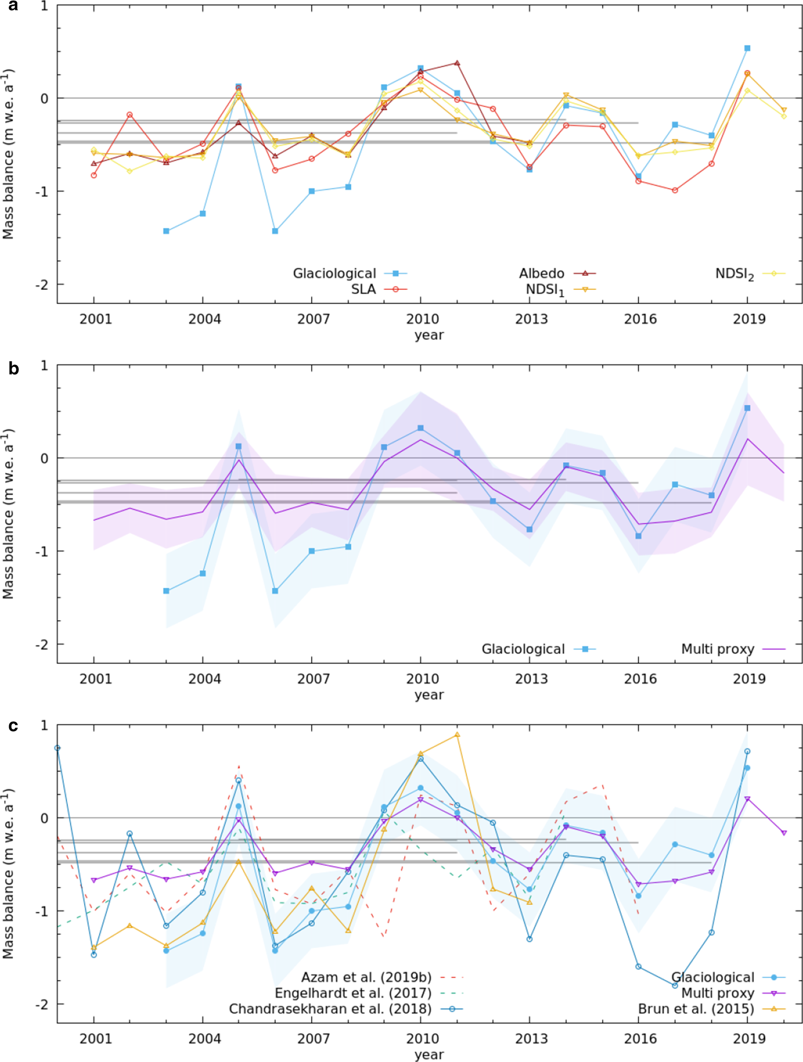
Fig. 4. (a) The reconstructed mass balance for individual proxies (solid lines+symbols) and the observed mass balance (blue symbo ls+line) on Chhota Shigri Glacier. The gray dashed lines are the available geodetic records. Error bars are omitted in this figure to minimise clutter. (b) The multi-proxy reconstructions (purple line) and the glaciological mass balance (blue line), with respective 1-σ uncertainty bands. (c) A comparison of the present multi-proxy reconstruction, previously reported reconstructions and glaciological mass balance. Model-based reconstructions are denoted by the dashed lines.
The multi-proxy reconstruction and the glaciological mass balance over the period 2003–2019 (Fig. 4b) had a high correlation (r = 0.86, ~p < 0.0001). The RMSE between the two time series was 0.39 m w.e. a−1, which was comparable to the uncertainty in the glaciological estimates. The mean reconstructed mass balance of −0.33 ± 0.22 m w.e. a−1 over the period was comparable to the corresponding glaciological mean of −0.46 ± 0.40 m w.e. a−1 within the uncertainty. However, the latter was more negative by 0.13 m w.e. a−1. The cumulative values of glaciological, reconstructed and geodetic mass balance for the periods corresponding to each of the available geodetic record are provided in Supplementary Table S2. The cumulative reconstructed and glaciological mass balances for the study period were −5.6 and −7.9 m w.e, i.e. the latter more negative by 2.3 m w.e. over the whole period. In contrast, the mean bias in the reconstructed mass balance with respect to the geodetic records was relatively small (−0.03 m w.e. a−1, equivalent of a cumulative bias of −0.5 m w.e over the period 2003–2019). As before, the reconstruction did not capture the highly negative glaciological mass-balance years before 2009, and had a comparably weaker interannual variability (Fig. 4c). The uncertainty in the reconstructed annual values in Chhota Shigri Glacier was in the range 0.09–0.38 m w.e. a−1, with a median value of 0.18 m w.e. a−1. This uncertainty was mostly due to the assumed noise in the geodetic records, followed by that in the minimum albedo records (Supplementary Fig. S3).
4.2. Saint-Sorlin and Argentière Glaciers
Using the proxies of NDSI1, NDSI2, minimum albedo and SLA, the present multi-proxy method produced reasonable annual mass-balance estimates of Argentière and Saint-Sorlin glaciers (Fig. 5, Supplementary Fig. S4). The corresponding cumulative reconstructed (glaciological) mass balances were −21.5(−24.8) m w.e. for Argentière Glacier, and −35.5(−38.9) m w.e. for Saint-Sorlin Glacier. The correlation coefficient, bias and RMSE of the reconstructed mass balance with respect to the corresponding glaciological values were 0.81 (p < 0.001), 0.16 m w.e. a−1 and 0.39 m w.e. a−1 for Argentière Glacier, and 0.90 (p < 0.001), 0.17 m w.e. a−1 and 0.43 m w.e. a−1 for Saint-Sorlin Glacier. The mean biases between reconstructed and geodetic mass balance records were negligible in comparison (−0.004 and −0.003 m w.e. a−1, respectively). The cumulative values of glaciological, reconstructed and geodetic mass balance for the periods corresponding to each of the available geodetic records are provided in Supplementary Tables S4 and S6. A somewhat subdued interannual variability of the reconstructed mass balance was apparent on these two glaciers as well (Fig. 5).
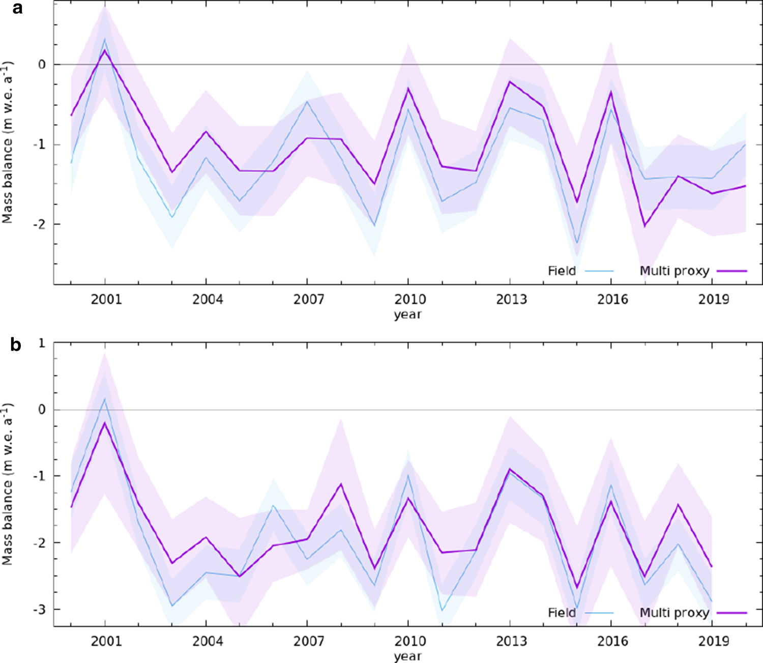
Fig. 5. The multi-proxy-reconstruction of annual mass balance (solid purple lines), and glaciological mass balance (solid blue lines) are shown for (a) Argentière and (b) Saint-Sorlin glaciers. The respective uncertainty bands are also shown (see text).
5. Discussion
5.1. Comparison with existing mass-balance reconstructions
It is clear from Fig. 4c and Table 1 that in terms of r and RMSE, the performance of the present multi-proxy method was comparable to that of the minimum albedo-based method (Brun and others, Reference Brun2015), and was better than that of the rest of the available reconstructions for Chhota Shigri Glacier. For the two glaciers in the Alps, RMSEs with respect to the corresponding glaciological records using the present method were comparable to that obtained in a previous reconstruction that was based on minimum albedo (Davaze and others, Reference Davaze2018). However, the authors calibrated their method using the glaciological records, which were not used at all in the present reconstruction. The previous SLA-based (Chandrasekharan and others, Reference Chandrasekharan, Ramsankaran, Pandit and Rabatel2018) or modelled (Engelhardt and others, Reference Engelhardt2017; Azam and others, Reference Azam2019) mass-balance time series for Chhota Shigri glacier yielded a relatively lower correlation (0.61–0.74) and a relatively larger RMSE (0.46–0.53 m w.e. a−1) (Table 1). Interestingly, the reconstructions based on SLA and minimum albedo obtained in the present study (Fig. 4a) matched well with each other on Chhota Shigri Glacier. In comparison, the previously reported reconstructions (Brun and others, Reference Brun2015; Chandrasekharan and others, Reference Chandrasekharan, Ramsankaran, Pandit and Rabatel2018) using the same proxy datasets showed large differences (Fig. 4c). Overall, a reasonable performance of the multiproxy reconstructions presented here for the Himalayan glacier and the two glaciers in the Alps indicated the utility of the method developed here. Particularly, the performance of the method on the relatively small Saint-Sorlin Glacier was encouraging.
Table 1. Correlation coefficient (r), RMSE and bias between the reconstructed and glaciological mass-balance estimates on Chhota Shigri Glacier.

The correlation coefficients are significant at p < 0.001 level, except for the last two rows, which are significant at p < 0.05 level
5.2. Biases in multi-proxy reconstructions
The reconstructed mass-balance time series for all the three studied glaciers showed a negligible mean bias in the range −0.03 to −0.003 m w.e. a−1 with respect to the geodetic data. However, the reconstructed balance was less negative by 0.13–0.17 m w.e. a−1 relative to the corresponding mean glaciological balance. For all the three glaciers, this bias was the same as that between the corresponding geodetic and glaciological mass-balance records (Fig. 6). Thus, the observed biases in the reconstructed mass-balance values with respect to the glaciological balance values were inherited from existing biases between the geodetic and glaciological mass-balance records for the glaciers studied, and were not artefacts of the reconstruction procedure. Such biases between geodetic and glaciological data are not uncommon, and geodetic data were previously used to bias correct the long-term glaciological mass balance in the Himalaya (e.g. Wagnon and others, Reference Wagnon2021) or in the Alps (e.g. Thibert and others, Reference Thibert, Blanc, Vincent and Eckert2008; Huss and others, Reference Huss, Bauder and Funk2009). Reconciling the above disagreement between the geodetic and glaciological data is not within the scope of the present study, which focuses on a method to disaggregate given decadal-scale geodetic mass-balance estimates to annual scale.

Fig. 6. A comparison between the available geodetic mass-balance records (b geo), and the mean glaciological mass balance (b gla) for the corresponding periods for the three studied glaciers (solid circles). The solid diagonal line denotes a hypothetical perfect match. On Saint-Sorlin Glacier, three records with large deviations (open circles) were ignored in the present study (see text for details).
5.3. Interannual variability of reconstructed mass balance
The reconstructed mass-balance time series for all the three studied glaciers had a somewhat lower interannual variability compared to that of the glaciological data (Fig. 4b). This may be related to a general tendency of most of the proxy-based methods to underestimate the mass loss for the years when the glaciological mass balance was highly negative. A saturation in the observed relationships between various proxies and the glaciological mass balance in the highly negative balance-years is well-known in the literature (e.g. Rabatel and others, Reference Rabatel2017). Also, a possible underestimation of the fit parameter β due to the systematic bias between the glaciological and geodetic mass balance on the studied glaciers could have contributed to the relatively smaller interannual variability.
5.4. A purely remote-sensing-based reconstruction
Compared to the existing proxy-based methods to estimate annual mass balance, the present method has an obvious advantage that it only requires geodetic data for calibration. Therefore, it can be applied to any given glacier where an annual time series of a set of proxies, and geodetic mass-balance records for more than one epoch are available. Here, there is no need for any glaciological mass-balance data. With several regional-scale datasets of glacier-specific geodetic mass balance being publicly available (e.g. Brun and others, Reference Brun, Berthier, Wagnon, Kaab and Treichler2017; Shean and others, Reference Shean2020; McNabb and others, Reference McNabb2021), the present method may potentially be applied to any glacierised region to estimate the glacier-wide annual mass balance. As the present method does not require any glaciological data, it may be particularly suited for data-sparse regions like the Himalaya and Karakoram.
We emphasise that the present method is not specific to the proxies used here, and can be adapted for any accessible linear proxy for the annual mass balance, without requiring any field data. However, the present reconstruction is contingent on a linear relationship (Eqn (2)) between the geodetic mass-balance values and the corresponding mean values of the proxies. This makes the reconstruction susceptible to possible noise and systematic biases in the geodetic data. For example, including the three geodetic records for Saint-Sorlin Glacier which were less negative compared to the remaining geodetic records and were therefore ignored (Supplementary Table S6) led to an unphysical fit to Eqn (2) for SLA with a negative best-fit β (Supplementary Fig. S5). Since the proxies are also correlated with the glaciological mass balance, any inconsistency or outliers within the set of available geodetic data may also be detected in a comparison between glaciological and geodetic records (Fig. 6).
5.5. Remote-sensing proxies
On Chhota Shigri Glacier, all the four proxies were highly correlated with the glaciological mass balance. These correlations were somewhat weaker than, but comparable to, the correlation between the glaciological data of ELA and mass balance (r = −0.94, ~p < 0.001) (Mandal and others, Reference Mandal2020). This suggests that the variability of these proxies faithfully reflects the annual mass balance. However, as discussed before, there were deviations from linearity and signs of saturation for some of the proxies (Fig. 3, Supplementary Figs S1, S2) for the highly negative mass-balance years. Such limitations of remotely-sensed proxies are well acknowledged in the literature (Rabatel and others, Reference Rabatel2017). While we do not offer any solution to such intrinsic issues related to the proxies, the strategy of combining multiple proxies may help in reducing the corresponding impact on the reconstructed mass balance.
The four proxies employed here were essentially based on the state of the snowcover on or around the glaciers as observed in optical and near-infrared satellite images. Consequently, they are susceptible to interference from cloud cover. This could limit the applicability of the multi-proxy method in certain climatic zones (Rabatel and others, Reference Rabatel2017). For instance, monsoon clouds often obscure the glacierised eastern Himalaya during summer, making it hard to obtain the proxy records themselves (Brun and others, Reference Brun2015). The four proxies employed here were associated with different parts of the glacier and the valley, and computed at different times of the ablation season. Estimating SLA involved measurements over a certain elevation band on the glacier at the end of the ablation season, e.g.the end of September for Chhota Shigri Glacier (Chandrasekharan and others, Reference Chandrasekharan, Ramsankaran, Pandit and Rabatel2018). In contrast, the minimum albedo was computed based on the average albedo over a larger fraction of the glacier surface, e.g. the accumulation zone and the upper ablation zone of Chhota Shigri Glacier (Brun and others, Reference Brun2015). Here, the timing of the occurrence of the minimum albedo was found to be mostly around the end of August and the beginning of September (Brun and others, Reference Brun2015). NDSI1 and NDSI2 were determined from the NDSI values averaged over a relatively large area around the glacier ablation zone, and were computed relatively early in ablation season – during the month of July. This strategy of combining multiple proxies based on the state of snowcover in different areas on and around the glacier and during different epochs of the ablation season, may in general be useful in obtaining a robust reconstruction by minimising possible data gaps. As the present method can incorporate any proxy that is linearly correlated with annual mass balance, possible novel proxies, e.g. those based on microwave remote sensing that can access the state of snowcover through clouds (e.g. Singh and others, Reference Singh, Tiwari, Gusain and Sood2020), may also be explored.
5.6. NDSI-based proxies
The strong correlations between glaciological mass balance and the two NDSI-based proxies for the month of July on the studied glaciers (Fig. 3, Supplementary Figs S2, S3) may be related to a sharp transition from an almost fully snow-covered to a mostly snow-free periglacial area around that time (Fig. 2). This is also the month with the highest air temperature on Chhota Shigri Glacier (Mandal and others, Reference Mandal2020). Therefore, a low July snowcover is likely to coincide with high ablation and/or low winter accumulation. In contrast, a high July snowcover over the periglacial area may indicate the presence of snow over the glacier, which suppresses melt due to a higher albedo. It is likely that these two proxies are not specific to the three glaciers studied, and could be useful for other glaciers as well provided there is no significant interference from cloud cover (Rabatel and others, Reference Rabatel2017). We acknowledge that in some cases there were signs of saturation in these proxies during the highly negative mass-balance years, when nearly all the periglacial area might have become snow-free. We also tested if the precise timing of the transition of the periglacial region from a ‘high-NDSI state’ to a ‘low-NDSI state’ (Fig. 2) could be used as a predictor of the annual balance. However, because of a high variability in the daily mean NDSI, the timing of the transition could not be ascertained accurately.
6. Conclusions
We developed a multi-proxy method to disaggregate the decadal-scale geodetic mass-balance measurements to annual scale on a given glacier where a set of linear proxies for annual mass balance is available. The method was applied to Chhota Shigri Glacier in the Indian Himalaya, and the Argentière and Saint-Sorlin glaciers in the French Alps. The reconstructions compared favourably with the corresponding field data, and with previously reported proxy- or model-based reconstructions. The use of multiple remotely-sensed proxies may make the method presented here robust against data gaps. Since the proxies and the data required for calibration involve only remote-sensing measurements, the method may be applied to any glacier provided a set of reliable proxies and accurate geodetic records are available. This is particularly advantageous for data-sparse regions like the Himalaya and Karakoram. Assessing the interannual variability of glacier-wide mass balance over a regional scale may lead to a better understanding of the corresponding interannual variability of the climate forcing, and that of the runoff of the glacierised catchments. However, any inherent bias in the geodetic records being disaggregated is propagated to the reconstructed annual mass-balance time series.
Supplementary material
The supplementary material for this article can be found at https://doi.org/10.1017/jog.2022.89
Data
All the data are provided in the Supplementary material. The codes for extracting the NDSI proxies and for performing the multiproxy reconstructions will be available at https://zenodo.org/record/7089006
Acknowledgements
We are grateful to Vijay and Braun (Reference Vijay and Braun2016), Brun and others (Reference Brun, Berthier, Wagnon, Kaab and Treichler2017), Shean and others (Reference Shean2020) and McNabb and others (Reference McNabb2021) for making their rich geodetic dataset public. We acknowledge Md Farooq Azam, A Chandrasekhar and M Engelhardt for sharing the modelled mass balance, A Chandrasekharan and R Ramshankaran for sharing the extended SLA records for Chhota Shigri Glacier, and Christian Vincent for sharing geodetic mass balance of Saint-Sorlin Glacier. For the studied glaciers in the Alps, the records of SLA Davaze and others (Reference Davaze, Rabatel, Dufour, Hugonnet and Arnaud2020) were from THEIA database (https://www.theia-land.fr/en/ceslist/glaciers-sec/), and the minimum albedo records were taken from Davaze and others (Reference Davaze2018). A.B. acknowledges discussions with M Barandun, E Berthier, F Brun, A Racoviteanu and S Vijay. We thank the anonymous reviewers of a previous version of the manuscript for useful suggestions. Valuable Inputs from an anonymous reviewer, reviewer A Rabatel, Scientific Editor F Brun, and Associate Chief Editor N Cullen are acknowledged. A.B. acknowledges support from grants NCAOR/2018/HiCOM/04 and MoES/PAMC/H&C/79/2016-PC-II.
Author contributions
A.B. conceived the study, came up with the multiproxy disaggregation method, did the analysis and wrote the paper. U.S. developed the NDSI-based proxies with help from A.B. U.S. and C.S. extracted the NDSI data, helped in the analysis, edited the manuscript and participated in the discussions.
Conflict of interest
None.


 Open access