


I. Introduction
Sea-ice remote sensing missions in the Arctic are constantly plagued by problems which reduce the yield of usable data significantly. The most serious of these problems is the generally poor weather found throughout the Arctic compounded by unreliable weather forecasts due to lack of weather stations in this remote region. The effectiveness of laser profilers, infrared scanners, and photographic cameras is especially reduced by inclement weather in study areas. Microwave systems, on the other hand, are not affected significantly by poor weather, and for this reason, appear to have the most potential for Arctic use.
Passive microwave instrumentation is simpler and less expensive than its active microwave counterpart, side-looking radar. The main disadvantage, however, is poorer resolution. In general, passive microwave remote-sensing techniques are especially attractive for Arctic sea-ice surveillance because of the minimization of possible sources of error and the provision of higher-quality quantitative results. The relative transparency of clouds and fog to microwaves and the independence of passive microwaves on solar illumination of the terrain, make passive microwave sensing a night and day, almost all-weather, technique. In the Arctic, the water-vapor constituent in the atmosphere is extremely low (on the order of 1 g cm-2 of precipitable water compared with 4.5 g cm2 for the equatorial regions). Such low values of atmospheric water vapor plus the low value of reflectivity (0.3 to 0.05) of the terrain (excluding water) makes the correction for the undesired reflected sky brightness temperature a minor one. Furthermore, extensive cloud cover with high liquid-water densities is not prevalent in the Arctic, making the corrections for atmospheric liquid water minor as well.
The Arctic terrain is also cooperative for passive microwave observations. The emissivity characteristics (and consequently the microwave brightness temperature) of the sea, ice, and snow as a function of frequency and polarization are markedly different at microwave frequencies compared with the infrared and visible regions. Within the microwave spectrum, the variations of emissivity as a function of frequency and polarization are comparatively large, and this makes a possible basis for unique identification of terrain features and surface description. Also, the Arctic sea-ice terrain is generally composed of large, relatively flat, homogeneous sources, which minimize the disadvantage of the poorer resolution and the possibility of immersing the side and main lobes in totally different ground sources of radiation.
During December 1973, the Naval Oceanographie Office (NAVOCEANO) and the Naval Research Laboratory (NRL) conducted a joint experiment over the sea-ice fields off Scoresby Sound on the east coast of Greenland using NAVOCEANO’s RP-3A Birdseye aircraft, laser profiler, and infrared scanner, and NRL’s 19.34 and 31.0 GHz nadir-looking microwave radiometers. The objectives of this mission were: (1) to develop skills for interpreting sea-ice passive microwave data, (2) to expand, if possible, the two-category capability of passive microwave sensors over sea ice, (3) to compare two frequencies (19 and 31 GHz) to determine which may be the more useful in a scanning radiometer (imager) now under development at NRL, and (4) to determine the value of multi-frequency as compared to single-frequency study of sea ice.
Earlier work has shown that multi-year ice provides a much lower microwave brightness temperature than does new or first-year ice (Reference WilheitWilheit and others, 1972; Reference GloersenGloersen and others, 1973; Kunzi and others, in press). However, a variety of conditions can exist within the instantaneous field of view of the microwave radiometer which can produce modified brightness temperatures of first-year and multi-year ice. It is also known that this response to ice types is a function of frequency. Therefore, the use of two nadir-looking radiometers at different frequencies capitalizes on the expected, measurable differences in brightness temperature as a function of frequency and ice types.
II. Instrumentation
A. Laser profiling system
The basic component of the laser profiling system is the continuous-wave laser altimeter manufactured by Spectra Physics, Inc., Mountain View, California. Basically, ranges are obtained by amplitude modulation of a helium-neon laser centered at 6 328 Å. The reflected light is detected and amplified by a photomultiplier and is phase compared with the modulation frequency of the transmitted beam. The phase difference is proportional to the transmission time or range. A Genisco Technology Corporation Reproducer Model 10-286 magnetic tape recorder and a Varian Statos I electrostatic strip-chart recorder were used to record the laser data. Jensen and Ruddock (unpublished) presented a detailed discussion of the laser profiling system.
B. Infrared scanning radiometer
The infrared (IR) system used in this experiment was modified by and obtained from the Naval Air Development Center, Johnsville, Pennsylvania. This instrument has a military designation of AN/AAR-35 and a commercial designation of Reconofax IV, Mark V, Infrared Scanner, manufactured by HRB-Singer Corporation. In this experiment, a mercury-doped germanium detector was used which has a spatial resolution of 17 mrad and a theoretical thermal resolution of 0.01 K at the nadir. Basically, the thermal map output of this instrument is produced by focusing the collected radiation with a rotating mirror (185 scans/s) onto the detector, which is filtered to accept wavelengths in the 8 to 14 μm region. The received radiation is then converted to voltages, which, in turn, are amplified and utilized to modulate the intensity of a crater lamp. The varying intensities of the crater lamp are recorded on 70 mm tri-x film, which, when developed, becomes the thermal map output (HRB-Singer, Inc., 1968).
C. Microwave radiometers
The NRL radiometers used on this experiment were conventional crystal-mixed, super-heterodyne, Dicke-switched radiometers that use an ambient (295 K) reference load in the switching cycle. The center frequencies were 19.34 GHz and 31.0 GHz with bandwidths of 10 to 300 MHz and 10 to 500 MHz, respectively. The r.m.s. output noise level is 0.3 K with a one-second integration time. In-flight calibration is achieved by observing a known input (ambient reference load for both halves of the switching cycle) and by injecting a calibrated temperature change generated by an argon noise generator. The reference-matched load temperature is known to within 0.5 K and the argon noise temperature change of 100 K is known to within 2%. The post-flight calibration, which determines the response of the receiver and the magnitude of the temperature injected by the argon noise generator, is performed using liquid nitrogen and ambient dewar-like loads that encircle the antennae.
A resolution of 38.0 m is achieved at an altitude of 305 m using antennae with beam widths of 7.2º. Beam efficiencies of the antennae are 87% at 19.3 GHz and 98% at 31.0 GHz.
Passive microwave radiometry provides quantitative results, but the quality of the data depends to a large extent on the nature of the calibration techniques as well as the quality of the equipment. The r.m.s. statistical error can be controlled fairly well by the selection of the r.f. components of the radiometer. The error in absolute measurement for the Dicke radiometer employed is dependent, in part, on the degree to which the observed source temperature differs from the temperature of the internal load used for reference. When these are equal, effects of the error inherent in the uncertainty of the injected argon calibration signal are minimized. In the case of Arctic ice, the temperature is displaced from the internal load by about 50 to 70 K. The systematic or bias error due to calibration error, error in load temperatures, and reduction errors is on the order of 2 K.
Although the data were recorded on both magnetic tape and analog strip charts, noise pick-up on the magnetic lape signal lines produced recordings of poor quality; consequently, only the analog data from the strip charts were used for analysis. The data were analog-recorded using a 0.25 s time constant or less with recorder chart speeds of 0.1, 0.5, and 1.0 inches per second (2.5, 1.27, and 25.4 mm s-1). A Benson Lehner Oscar k data reader was used to digitize the analog data automatically for computer reduction to brightness temperature. These calculations took into account the calibration data, reference-load temperature, beam efficiency as a function of antenna angular extent, expected response from the ground source as a function of angle, and atmospheric corrections as a function of incidence angle. Surface temperature provided by a weather station in Iceland was ( —20±2)° C which is consistent with the accuracy of the temperature recorded outside the aircraft over the site of ( — 27±2)°C recorded at 1 525 m and of (—20±2) ° C recorded at 150 m. This temperature is also consistent with that expected for lat. 70° N., based on an Arctic model atmosphere for winter.
III. Results
Since there were no in situ ground-truth measurements made during this experiment, the key to meeting the mission’s objectives was the ability to identify accurately several different ice types using remote sensors other than the passive microwave radiometers. Since light conditions were insufficient to allow photographic imaging of the sea ice, it was necessary to rely solely on laser and infrared data for this identification. Fortunately, these two systems provided excellent data allowing the identification of six distinct ice types (based on age) or ice forms (based on surface roughness) with a high degree of confidence; they are: (1) open water/new ice, (2) young ice or thin, smooth, first-year ice, (3) thick, smooth, first-year ice, (4) ridged first-year ice, (5) smooth multi-year ice, and (6) rough multi-year ice. In most cases, the young ice and thin, smooth, first-year ice of (2) above could be differentiated on the basis of the amount of reflection of the laser signal from the ice surface, but, the difference was not as obvious as with the other categories. To illustrate the typical laser/IR signatures of these ice types, Figures 1 through 4 are presented. On these, and in subsequent illustrations where infrared imagery is presented, lighter shades of gray represent warmer surface temperatures with respect to the surrounding ice conditions. Since water is the main source of heal for the ice at this time of year, thinner ice types are usually warmer than thicker ones and thus appear lighter. The laser profiler is an active system measuring the reflected laser beam, hence surface reflectivity is an important key for proper interpretation. The low reflectivity of thin ice and open water results in a low signal-to-noise ratio, and a relatively noisy profile is obtained from these surfaces. On the other hand, first-year and older ice usually has a snow cover, and the associated high surface reflectivity produces a sharp, low-noise profile. The distinction between first-year ice and multi-year ice can easily be made using the characteristics of their profiles. First-year ice is typically Hal, broken by periodic steep-sided pressure ridges. Multi-year ice, on the other hand, has undergone two or more summers of melt and the steep-sided pressure ridges have been eroded so that an undulating terrain results. Ketchum (1971) and Reference Ketchum and WittmannKetchum and Wittmann (1966) present complete descriptions of laser and IR interpretation techniques of Arctic sea ice.
Figure 1 presents a section of open water/new ice. This ice type is extremely thin and appears very warm on the IR image. The laser profile is very flat and noisy. (Aircraft motion has not been removed from the laser data presented in this paper. Therefore, some long-wave curvature may be present in the profiles.)

Fig. 1. Infrared image and laser profite for open mater/new ice.
Figure 2 presents the three forms of first-year ice identified on this study using laser and IR data. On the left is thick, smooth, first-year ice. The IR image of this ice is fairly dark in tone due to its thickness with some darker lineations due to snow drifts and some infrequent ridges. Since this ice type does have a snow cover, the laser profile is not noisy, and because the ice is smooth, the profile is very flat. The middle portion of Figure 2 shows thin, smooth, first-year ice or young ice. The IR image shows the ice to be thinner (lighter in tone) than the thick first-year ice to the left, and the laser profile is flat (undeformed) and noisy (no snow cover). The deformed first-year ice on the right of this figure is easily identified on the laser profile by the number of spikey-looking pressure ridges or blocks of broken ice. The IR image is similar to the thick smooth ice except that the ridged ice has a more mottled appearance.
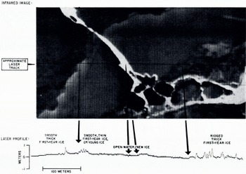
Fig. 2. Infrared images and laser profiles, for thin, smooth first-year ice. thick, smooth first-year ice, and ridged, thick first-tear.
Figure 3 presents a section of relatively smooth multi-year ice. The laser profile is typical for multi-year ice; i.e. high signal-to-noise ratio and undulating terrain with periodic broad-based hummocks and pressure ridges. The IR image is dark in tone and generally nondescript with the exception of some lineations due to pressure ridges and some mottling due to hummocks.

Fig. 3. Infrared innige und laser profile for smooth multi-year ice.
The rough multi-year ice presented in Figure 4 has a similar laser profile to the smooth multi-year ice, but upon closer examination it is quite apparent that this ice has many more hummocks and ridges than the ice shown in Figure 3. In addition, the features have steeper sides. The IR image is more mottled than that for smooth multi-year ice.
Several hundred kilometres of data were collected on this mission. From this large amount of data, five small sections (ranging from 7 to 26 km each) were selected for detailed study. Each of these five sections comprised one or more unique features, such as large areas of homogeneous first-year ice, large multi-year ice floes, large open-water/new-ice areas, recently deformed, highly broken ice, etc. Since the three data forms (laser, IR, and passive microwave) had a common time base, it was a simple matter to correlate the three for comparison.
Comparison of the dual-channel passive microwave results with the laser/IR results indicate that multiple, identifiable surface responses other than the expected, simple bimodal response exist. Description of the surface can be expressed using the average of the results at the two frequencies plotted against their difference at the two frequencies (e.g. Fig. 5). Such plots can be used to identify first-year, multi-year, and open water/new ice. The plots also show, however, that there is a wide range of responses for ice surfaces that is well beyond system variations. There appear to be two regions of first-year ice, a region of higher brightness temperature (245 K) and a region of lower brightness temperature (approximately 235 K). The former could usually be correlated with ridged first-year ice and the latter with smooth first-year ice. Also, two forms of multi-year ice were observed using the passive microwave radiometers, a region of higher brightness temperature (generally above 190 K) with smaller temperature differences between frequencies (about 20 K) and a region of lower brightness temperature (less than 190 K) with larger temperature differences (about 30 K). Although no direct remote-sensing or ground-truth proof exists, the higher temperature form is interpreted as second-year ice and the lower temperature form as multi-year ice.
It appears that dual-frequency passive microwave techniques may have possible use in identifying five ice types and/or ice forms: (1) open water/new ice, (2) smooth first-year ice, (3) ridged first-year ice, (4) multi-year ice, and (5) a higher radiometric temperature form of multi-year ice hypothesized as second-year ice.
On Figure 5 the general location of each of the five ice types is indicated on an idealized diagram of average brightness temperature at the two frequencies versus the difference in temperature between the two frequencies (that at 19.3 minus 31.0 GHz). Open water/new ice stands alone with a relatively cool radiometric temperature and a large negative temperature difference due to the strong negative response by the longer wavelength 19.3 GHz radiometer. This result has been observed by previous investigators.
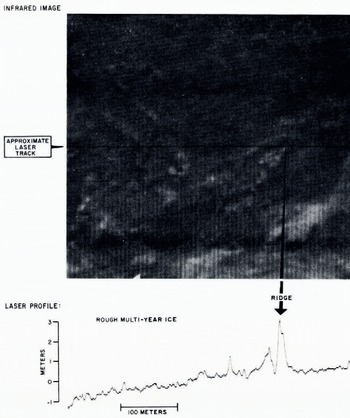
Fig. 5. Idealized diagram depicting the general areas of homogeneous ice form delineated by dual-frequency passive microwave radiometry.
On this experiment it was possible to subdivide first-year ice into two categories based on surface roughness as mentioned above. Previous studies have shown first-year ice to be frequency independent. This independence was also observed here as indicated by the near-zero value for temperature difference. Adjacent sections of smooth first-year ice of different thicknesses (as determined from IR data) were found to have the same brightness temperature. Therefore ice thickness, or age of first-year ice, did not appear to affect microwave radiometric temperature.
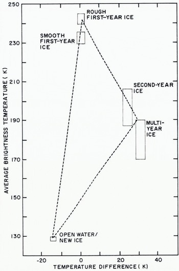
Fig. 4. Infrared image and laxer profile for rough multi-year ice.
Probably the most surprising result of this experiment was the ability of passive microwave to distinguish two distinct forms of multi-year ice. Surface roughness did not appear to have any effect on the brightness temperature of the two multi-year ice forms. It is more likely that internal structure is responsible for this delineation. The air-bubble argument of Poe and others (1974) states that multi-year ice should have larger air bubbles than second-year ice, hence it will have a larger correlation length and a lower emissivity.
Another feature which Figure 5 emphasizes is the large variations in temperature and temperature difference possible for both forms of multi-year ice for any one floe. Figure 6 presents a radar image of such a floe collected by the U.S. Coast. Guard in the summer of 1969. From this figure, it is clear that a multi-year ice floe is far from homogeneous, but rather a conglomerate of many smaller pieces of ice of varying ages and thicknesses, re-frozen melt ponds, and drainage patterns formed from summer melt.

Fig. 6. U.S. Coast Guard side-looking radar image depicting inhomogeneity characteristic of multi-year ice-floe.
Figure 5, as stated above, is an idealized diagram representing typical values for homogeneous or near-homogeneous sections of ice. The sea-ice canopy, especially in the marginal ice zones, is extremely dynamic, leaving only a small number of uniform ice sections. What happens to a diagram of the kind idealized in Figure 5 over more complex ice conditions depends un what types of ice are in the beam spot (38.0 m) at any one particular time. Therefore, beam-smoothing or averaging ran produce data points anywhere along the perimeter of the dashed triangle, for example, should the terrain be a combination of first-year ice and open water, (i) temperature differences will lend toward the negative because the radiometric temperature of water at 19.3 GHz is much lower than it is at 31.0 GHz, and (ii) average temperature will fall somewhere along the line joining first-year ice and open water/new ice depending on the percentage of each type within the beam spot. The concept of Figure 5 can be used to provide an all-weather method of describing an ice field with respect to ice type and roughness.
Figure 7 presents data for one of the five sections selected for detailed analysis. This section, which is approximately 22 km long, had significant areas of all of the five ice types distinguishable by passive microwave radiometry except open water/new ice. Many data points stray from the perimeter of the triangle, however, the density of data points in various areas clearly indicate the predominant ice forms present.

Fig. 7. Plot of average brightness temperature versus temperature difference for 22 km section.
Figure 8 was compiled from a short run (11 km) comprised mostly of ridged first-year ice and second-year ice. Two well-defined, dense areas appear on Figure 8 corresponding to rough first-year and second-year ice as shown on Figure 5 above.

Fig. 8. Plot of average brightness temperature versus temperature difference for 11 km section.
Figures 9, 10, and 11 present specific examples of passive microwave responses to various changes in ice. Figure 9, which shows three types (smooth first-year, multi-year, and second-year ice) is presented primarily lo show the difference between second-year and multi-year ice. Multi-year ice is characterized by lower temperatures and greater temperature differences than those found for second-year ice.

Fig. 9. Infrared images and passive microwave profiles for possible second-year ice. multi-year ice. and smooth first-year ice.

Fig. 10. Infrared images and passive microwave profiles for smooth first-year ice and ridged first-year ice.
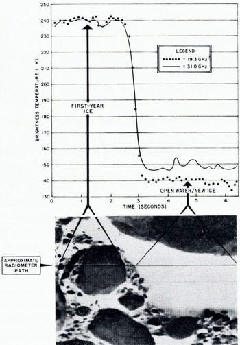
Fig. 11. Infrared images and passive microwave profiles for first-year ice arid open water/new ice.
Figure 10 shows the subtle difference in microwave radiometric temperature between smooth first-year and rougher first-year ice (the roughness being determined from the laser profile). Both frequencies respond in a similar fashion, but radiometric temperature shows a definite response for the very smooth ice sensed by the radiometer.
Figure 11 is an example of the response of passive microwave lo open water/new ice. This signature has been reported by previous investigators (e.g. Gloersen and others, 1973)·
Summary
Using two frequencies, passive microwave appears capable of distinguishing between five distinct ice types and forms: (1) open water/new ice, (2) smooth first-year ice, (3) ridged first-year ice, (4) multi-year ice, and (5) second-year ice. Delineation between the first-year ice forms (2) and (3) above, seemed to be independent of age or thickness, but to depend rather on surface roughness. The broad-based ridges and hummocks of multi-year ice on the other hand, did not appear to influence brightness temperature by any significant amount; rough multi-year ice was observed to have the same radiometric temperatures as smooth multi-year ice. Instead, internal structure (specifically air bubbles) may be responsible for the delineation of a higher-temperature multi-year ice form hypothesized as second-year ice.
The 30 K range in brightness temperature observed for multi-year ice is probably attributable to the inhomogeneity of multi-year ice caused by its make-up of ice of various ages and from surface irregularities created by summer melt.
By plotting average brightness temperature versus temperature difference, it appears possible to describe the ice field generally in terms of the five categories listed above regardless of weather conditions.
A mixture of first-year and multi-year ice within the beam spot can produce the observed deviations, but other mechanisms not discussed in this paper might also be responsible:
-
Patches of surface temperature in excess of the 253 K used in reducing brightness temperature,
-
Heating differentials due to patches of snow cover,
-
Heating differentials due to the insulating effects of cloud cover, and
-
Temperature differentials due to undetected areas of thin ice.
However, the consistency of the microwave values for any one floe, and the uniform and consistent weather experienced during the flight, appear to preclude the above list from serious consideration. Instead, most variations of the data points from the areas indicated on Figure 5 are probably due to beam smoothing at the boundaries of differing ice types.
Since microwave systems are not affected significantly by poor weather conditions, they appear to have a high potential for Arctic use. The relative transparency of clouds and fog to microwaves, and the independence of passive microwaves of solar illumination or artificial illumination of the terrain, make passive microwave sensing a night-and-day, almost all-weather, technique. Furthermore, the relatively inexpensive instrumentation, and simple requirements for data interpretation, make passive microwave attractive on an operational basis.
Discussion
P. GLOERSEN: TWO questions on your suggested sub-categories for first-year and multi-year ice. (a) The example shown for first-year ice seemed to have an open lead running along the aircraft track. Could this account for the slightly lower TB observed? (b) Is it possible that the two sub-types of multi-year ice might correspond to different snow accumulations on the two floes ?
S. G. TOOMA: (a) I admit that the example shown was a poor choice. There are small thin ice areas present which could account for the drop in temperature. However, there are many other areas which do show the same drop in temperature without thin ice being present. (b) Yes, it is possible.
A. W. ENGLAND: HOW thick was your “open water/new ice”
TOOMA: About 5 cm.
ENGLAND: Your data are consistent with the results from our theoretical modelling. For open water/new ice, the longer wavelength "sees" through the ice and the colder-seeming water results in colder (longer wavelength) brightness temperatures, First-year ice contains brine causing strong frequency-independent absorption. The brightness temperature will be the same at both wavelengths. The brine has drained from multi-year ice so that the absorption is lower and there is greater penetration. The empty brine pockets act as scatterers affecting preferentially the shorter wavelengths. Therefore, scattering, older ice will appear darker at shorter wavelengths.
W. F. WSEEKS AND J. F. NYE: HOW hopeful are you of using this type of system to distinguish different classes of thin ice? The reason for the question is that in current models of the mechanical behaviour of pack ice it is the thickness distribution of thin ice that is the important parameter that we must measure.
TOOMA: I realize the importance of the thickness distribution, but I am not hopeful at this time that we will be able to distinguish many different classes of thin ice.


