


1. Introduction
The Tibetan Plateau (TP), which is one of the regions with the highest glacier concentration outside the polar region, is the source region of all the large rivers in Asia (Immerzeel and others, Reference Immerzeel, van Beek and Bierkens2010; Yao and others, Reference Yao2012; Zhang and others, Reference Zhang, Jiang, Liu, Sun and Wang2018). Impacted by climate warming, most of the glaciers on the TP have undergone great mass loss over the past 30 years, which may lead to unsustainable water supplies for major rivers and threaten the livelihoods of people in the downstream regions (Kang and others, Reference Kang2010; Yao and others, Reference Yao2012; Liang and others, Reference Liang, Cuo and Liu2019). The best way to understand how climate perturbations impact the status of glaciers is to monitor glacier changes (Immerzeel and others, Reference Immerzeel2014; Paul and others, Reference Paul2015). However, the field observations of TP glaciers remain scarce due to inaccessibility, the harsh climate and the high cost (Rossini and others, Reference Rossini2018; Zhang and others, Reference Zhang, Jiang, Liu, Sun and Wang2018).
Satellite remote sensing measurements of glacier changes complement field observations. In particular, Landsat imagery with long time series archives has been proven an efficient tool for mapping glacier areas and monitoring glacier changes, even for small glaciers (Kääb and others, Reference Kääb, Paul, Maisch, Hoelzle and Haeberli2002; Paul and others, Reference Paul, Kääb, Maisch, Kellenberger and Haeberli2002; Andreassen and others, Reference Andreassen, Paul, Kääb and Hausberg2008; Fischer and others, Reference Fischer, Seiser, Stocker Waldhuber, Mitterer and Abermann2015). Existing methods using multispectral images to outline boundaries for debris-free glaciers are mature (Paul and others, Reference Paul2015). However, most satellite data still present some fundamental challenges for glacier monitoring, such as low spatiotemporal resolution and high cost (Whitehead and others, Reference Whitehead, Moorman and Hugenholtz2013). Additionally, cloud cover is a notable issue in the mountain regions (Wigmore and Mark, Reference Wigmore and Mark2017).
Uncrewed aerial vehicles (UAVs) have a history in military applications (Vallet and others, Reference Vallet, Panissod, Strecha and Tracol2011). In the last two decades, this technology has been applied in the civil domain and has created a new remote sensing market (Colomina and Molina, Reference Colomina and Molina2014). UAV technology can make up for the shortcomings of satellite remote sensing and traditional surveys. It is now possible to acquire both high-resolution orthomosaics and topography of targets using photogrammetric software and a consumer-grade camera that is mounted on a lightweight UAV. Currently, the use of UAVs in the field of earth science is undergoing rapid expansion because of the ultra-high spatiotemporal resolution and low-cost benefits of UAV technology (Kraaijenbrink and others, Reference Kraaijenbrink, Shea, Pellicciotti, de Jong and Immerzeel2016b; Wigmore and Mark, Reference Wigmore and Mark2017; Zmarz and others, Reference Zmarz2018; Carrera-Hernández and others, Reference Carrera-Hernández, Levresse and Lacan2020; Giordan and others, Reference Giordan2020). Nevertheless, UAV-based glaciology research is a very small part of all UAV-based environmental research.
In glaciology, the first published paper of UAV applications focused on the polar region (Hodson and others, Reference Hodson2007), and such interest has continued to grow. Subsequently, UAV technology has been successfully applied in research on Himalayan and Alpine glaciers. For example, Immerzeel and others (Reference Immerzeel2014) performed three UAV surveys on a debris-covered Himalayan glacier for the first time and indicated that UAV technology may revolutionize classical field-based methods; Benoit and others (Reference Benoit2019) conducted ten UAV surveys on an Alpine glacier without GCPs; they extracted the coordinates of the bedrocks around the glacier from one survey product and used them to co-register the remaining products. However, the number of studies on UAV-based high mountain glaciers is low compared with the alpine and polar regions, especially for those mountain glaciers on the TP. To our knowledge, current research on UAV-based high mountain glaciers only involves five TP glaciers. They are Changeri Nup glacier (Vincent and others, Reference Vincent2016; Brun and others, Reference Brun2018), Langtang glacier (Kraaijenbrink and others, Reference Kraaijenbrink, Shea, Pellicciotti, de Jong and Immerzeel2016b), Lirung glacier (Immerzeel and others, Reference Immerzeel2014; Brun and others, Reference Brun2016; Buri and others, Reference Buri, Pellicciotti, Steiner, Miles and Immerzeel2016; Kraaijenbrink and others, Reference Kraaijenbrink2016a, Reference Kraaijenbrink2018), Baishui River No. 1 glacier (Che and others, Reference Che, Wang, Yi, Wei and Cai2020) and Parlung No. 4 glacier (Yang and others, Reference Yang2020). Moreover, these five glaciers are all distributed in the south and southeast TP. Little glacier research on the central TP has included UAV deployment.
In this paper, four high-resolution UAV surveys were conducted over Xiao Dongkemadi (XDKMD) Glacier and Ganglongjiama (GLJM) Glacier in 2017 and 2019 to obtain glacier changes in the short term. Additionally, we utilized several Landsat scenes to depict changes in the two glaciers over the last 30 years and chose a 10-year interval between two selected images due to the coarse spatial resolution. The main objectives of this study were (1) to apply a UAV for central TP glaciers and verify its feasibility and (2) to shed light on the long- and short-term changes in XDKMD Glacier and GLJM Glacier.
2. Study area
XDKMD Glacier (33°04′N, 92°04′E) and GLJM Glacier (33°34′N, 91°12′E) are located in the Tanggula Mountains of the central TP (Fig. 1). Both glaciers are typical continental glaciers in the Yangtze River source region (Zhang and others, Reference Zhang, Jiang, Liu, Sun and Wang2018) and have a mean elevation that exceeds 5000 m above sea level (a.s.l.). The climate in this region is mainly influenced by the westerlies and monsoons. Thus, it presents cold, arid, windy winters and warm, wet summers (Liang and others, Reference Liang, Cuo and Liu2019), that is, precipitation mainly occurs in summer when the temperature is high. Therefore, the most dynamic season, when the accumulation and ablation processes of glaciers occur synchronously, is summer (i.e. from June to September, hereafter referred to as the ablation season).
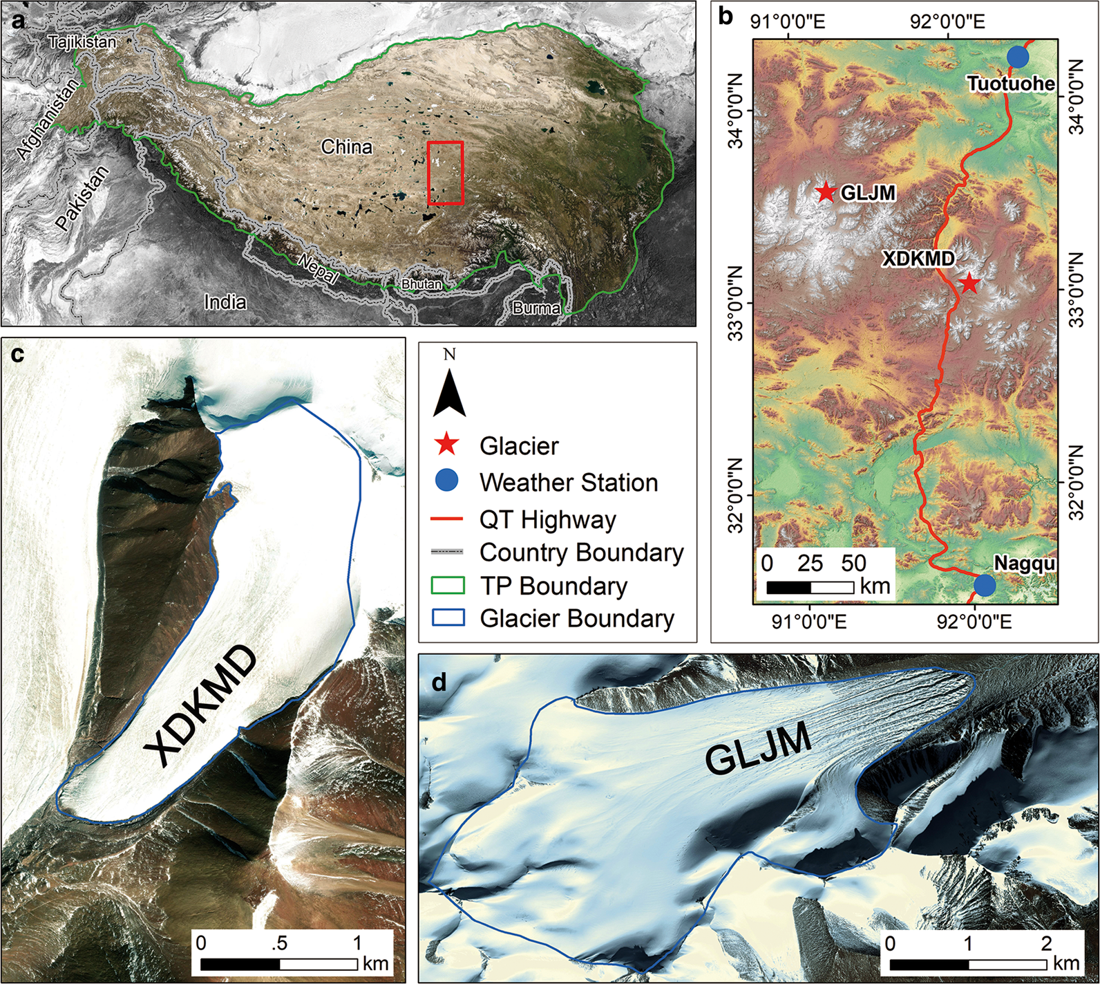
Fig. 1. Overview of the study area. (a) Extent of the TP; our study sites are on the central TP. (b) Details of our study sites. (c) Aerial view of XDKMD Glacier (source: Esri, Maxar). (d) Aerial view of GLJM Glacier (source: Bing Maps). Both glacier boundaries are obtained from CGI-2 (Guo and others, Reference Guo2015).
XDKMD Glacier is a southwest-facing tributary glacier, with an area of 1.705 km2; its terminal altitude changed from 5380 m in 1996 to 5420 m in 2013 (Zhang and others, Reference Zhang, He, Ye and Wu2013). XDKMD Glacier has been observed since 1989 (Pu and others, Reference Pu2008), and an observation station was built in 2005 beside Qinghai-Tibet Highway. The travel time from the station to XDKMD Glacier is approximately two hours. The station now has relatively long-term records of mass balance of XDKMD Glacier, which are the second longest after Urumqi Glacier No. 1 in High Mountain Asia (Pu and others, Reference Pu2008; Zhang and others, Reference Zhang, He, Ye and Wu2013).
GLJM Glacier is located in the northeast corner of Geladaindong, which is a nature reserve in the Yangtze River source region (Ye and others, Reference Ye, Kang, Chen and Wang2006). According to the Second Chinese Glacier Inventory, the GLJM Glacier area in 2007 was 12.3 km2, with a maximum altitude of 6106 m and a minimum altitude of 5224 m (Guo and others, Reference Guo2015). The field observations of GLJM Glacier, which are challenging, started in 2017. As the travel time from the station to the GLJM Glacier is ~1 d, we need to camp there without a mobile signal for a few days to finish our fieldwork. The terminal surface of GLJM Glacier is very broken and forms some erosional features (Fig. 2a). Meltwater flows from the glacier and forms a river at the terminus. A thick layer of ice forms on this river and melts gradually during the ablation season (Fig. 2b).
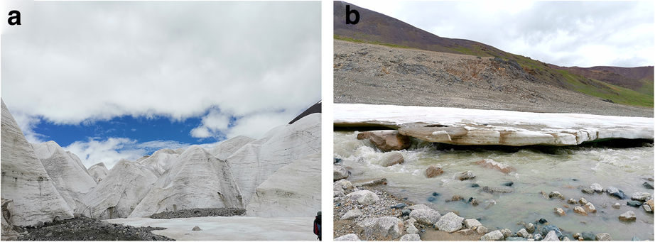
Fig. 2. Photos of GLJM Glacier taken in July. (a) Erosional features in the terminus of GLJM Glacier. (b) The ice on the glacier terminal river.
3. Data and methodology
3.1 Landsat imagery
Currently, the publicly available remote sensing data commonly used for glacier delineation are Landsat and Sentinel-2. Landsat data have a longer time series; the resolution of visible, near-infrared (NIR) and short-wave infrared (SWIR) bands can be improved to 15 m after pan-sharpening (Landsat 7/8). Sentinel-2 data have a resolution of 10 m in visible and NIR bands, but a resolution of 20 m in SWIR band. Consider the method we used (NIR/SWIR), we could get higher resolution results with Landsat data. Therefore, we selected eight optimal Landsat scenes from 1988 to 2018 based on the cloud and snow cover conditions, with an image interval of 10 years. Additionally, another two scenes in 2017 and 2019 were selected for the comparison of the outlines from the UAV and Landsat (Table 1). All the scenes were provided by United States Geological Survey (USGS) (https://earthexplorer.usgs.gov) and orthorectified automatically by USGS using SRTM3 DEM (level 1 T). According to the research of Guo and others (Reference Guo, Liu, Xu, Wei and Ding2012), Landsat data have high precision, and most of them have correction accuracies of approximately half a pixel or more.
Table 1. Utilized Landsat scenes
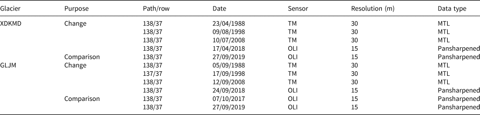
In the seventh column, MTL means multispectral and Pansharpened means the fused image of panchromatic and multispectral images.
3.2 UAV surveys
In this study, a DJI Phantom 4 Pro quadcopter UAV was employed to conduct four surveys on the ablation zone of XDKMD Glacier and GLJM Glacier during the ablation season (refer to Table 2). The Phantom 4 Pro is equipped with a 20 MP digital compact camera with a built-in, three-axis stabilization system. With a 1.388 kg ultra-light body, the UAV is capable of ~30 min of flight at a speed of 50 kph in positioning mode (DJI, 2017). However, the battery conversion rate will be greatly reduced in cold, low-pressure and high-altitude conditions, and the maximum tested photographing time with one battery is 15 min when the UAV takes off above 5000 m a.s.l.
Table 2. Overview of the UAV campaigns performed in the ablation zone of the two study glaciers
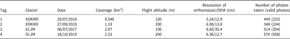
The details of these surveys are shown in Figure 3. The UAV flew automatically along the flight course predefined by Pix4Dcapture (https://www.pix4d.com/product/pix4dcapture) and took photographs at a certain time interval. The position and attitude of the UAV at the exposure stations, which were obtained by the built-in integrated Position and Orientation System (POS, composed of global positioning system and inertial measurement units), were recorded in the JPEG pictures. However, we discovered that the altitude error of the final products exceeded 200 m without GCPs in the first survey of XDKMD Glacier, and thus, we set up four and three GCPs to improve the accuracy in the following surveys in September and October, respectively. The GCPs were composed of 1.5 by 1.5 m of red waterproof cloths with a yellow cross in the center distributed on the lateral moraine and glacier surface. The coordinates of the centers of the markers were measured using a Trimble GeoXT handheld GPS receiver, which can provide sub-meter accuracy with real-time or post-processed differential correction.
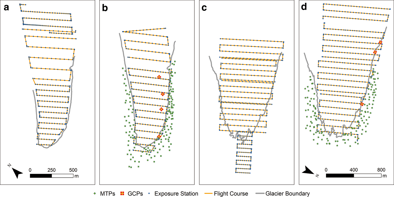
Fig. 3. Flight course of four UAV surveys: (a) 20/07/2019 in XDKMD Glacier, (b) 27/09/2019 in XDKMD Glacier, (c) 06/07/2017 in GLJM Glacier, (d) 16/10/2019 in GLJM Glacier.
3.3 UAV data processing
UAV images in each survey were separately processed with Pix4Dmapper (Pix4D) in a three-step workflow, which is described below:
(1) Initial processing: This process generates a sparse point cloud with the structure-from motion algorithm (Turner and others, Reference Turner, Lucieer and Watson2012). First, it searches for and matches key points in the photos that have certain overlapping areas using a feature matching algorithm (e.g. the scale-invariant feature transform (SIFT) algorithm, which can detect key points in photos with different views and illumination conditions; Lowe, Reference Lowe1999, Reference Lowe2004). Second, the approximate locations and orientations of the camera at each exposure station are reconstructed with the internal parameters (focal length, coordinates of the principal point of the photograph), and external parameters (i.e. POS data). A sparse point cloud is created.
(2) Point cloud densification: In this step, the multi-view stereo technique is applied to achieve a higher point cloud density than in the previous step (Furukawa and Ponce, Reference Furukawa and Ponce2010; Mölg and Bolch, Reference Mölg and Bolch2017). Thus, the spatial resolution of the products can be increased, and an irregular network for the next step can be created (Küng and others, Reference Küng2012).
(3) Digital elevation model (DEM) and orthomosaic generation: DEM and orthomosaic are the two main final products. DEM can be built from dense point cloud or irregular network, and the former one usually has higher accuracy for rugged terrain. Every image pixel is projected on DEM and the georeferenced orthomosaic is generated (Küng and others, Reference Küng2012).
During this process, we found photos with too much snow coverage that cannot be matched, that is, few feature points can be detected and matched in those photos, especially in survey 1, where almost half of the photos are invalid (Table 2). These issues also occur in the landscape with a homogeneous surface (e.g. still water) as these surface features do not provide enough of the visible attributes needed for algorithms such as SIFT (Harwin and Lucieer, Reference Harwin and Lucieer2012).
We did not set GCPs in surveys 1 and 3, and the GCPs in surveys 2 and 4 were not well distributed. Thus, to accurately identify changes in the glaciers from the UAV images, the products of surveys 1 and 3 (Table 2, first column) need to be co-registered to the references of surveys 2 and 4 (Immerzeel and others, Reference Immerzeel2014; Benoit and others, Reference Benoit2019). Figure 4b illustrates the workflow of co-registration process. Consider the XDKMD Glacier, for example. First, we processed the data from surveys 1 and 2 to obtain the final products. We compared their orthomosaics to find some stable, well-marked surface features as manual tie points (MTPs). Second, we extracted the MTPs coordinates from the products of survey 1 and applied them as GCPs to reprocess the data from survey 2. Last, we obtained co-registered products of survey 2. Thus, the products at different times could be overlapped and the change of XDKMD Glacier could be detected.
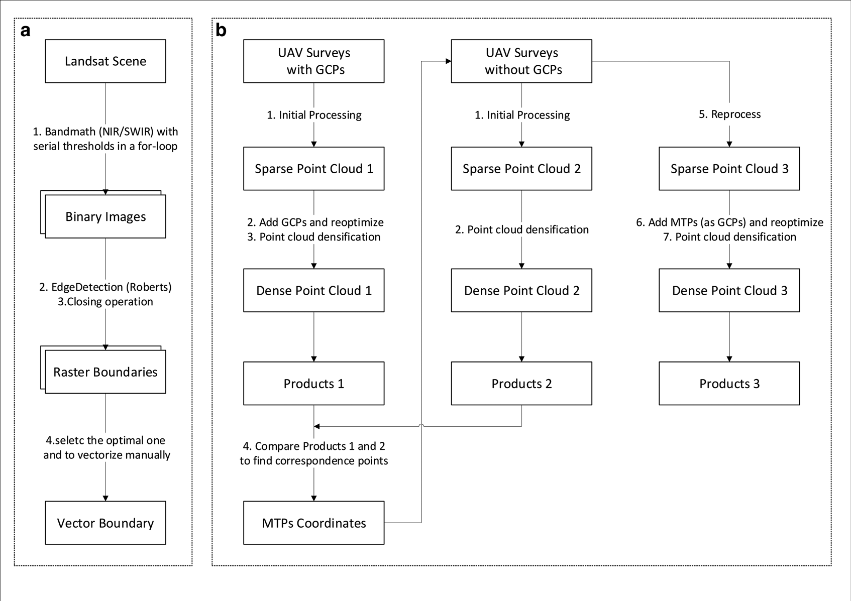
Fig. 4. Workflows of glacier delineation (a) and how we co-register the UAV data (b).
The MTPs utilized for the co-registration are mostly bedrocks and boulders with a width range of 1–3 m. To further confirm that the selected MTPs are stable, we need to check that the size, shape and surrounding features (e.g. stone, riverway) of these MTPs are the same between two repeated surveys. The geographic coordinates of the MTPs can be easily extracted in the pix4Dmapper. And in the end, we selected 143 MTPs and 136 MTPs from the products of survey 2 and survey 4, respectively.
3.4 Glacier delineation
3.4.1 Landsat
Previous studies have suggested that one of the most effective methods for glacier mapping is NIR/SWIR band ratio, which utilizes the large difference in spectral signature between snow and other materials in these spectral bands (Andreassen and others, Reference Andreassen, Paul, Kääb and Hausberg2008; Bolch and others, Reference Bolch2010). The whole process is implemented via automatic batch processing based on programming (Fig. 4a). For one Landsat scene, first, a ‘ratio image’ is computed from the raw digital numbers for bands NIR/SWIR, and several different binary images are generated by setting a sequence of empirical thresholds (from 1.5 to 2.5, step size of 0.1; Fig. 5). Second, the raster boundaries with different thresholds are generated via edge detection (Roberts Operation) and denoised by the closing operation. Last, we select the best matching boundary for every scene to vectorize them manually. Thus, the change in the glacier margins is depicted in the overlay map using different polygons. Additionally, the method of drawing profile lines (Fig. 6) in different directions on the glacier terminus is adopted to compare the terminus changes and calculate the average rate of glacier retreat (Li and others, Reference Li, Sun and Zeng1998; Cao and others, Reference Cao, Li, Chen, Wang and Che2006).
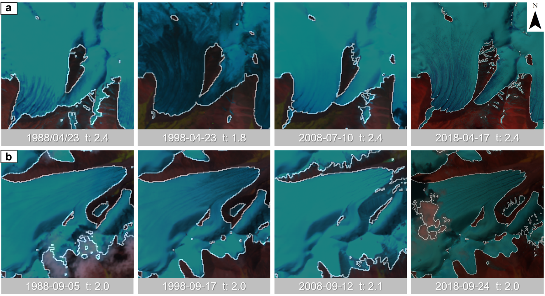
Fig. 5. Optimal threshold (t) that we selected for each Landsat scene of XDKMD Glacier (group A) and GLJM Glacier (group B).
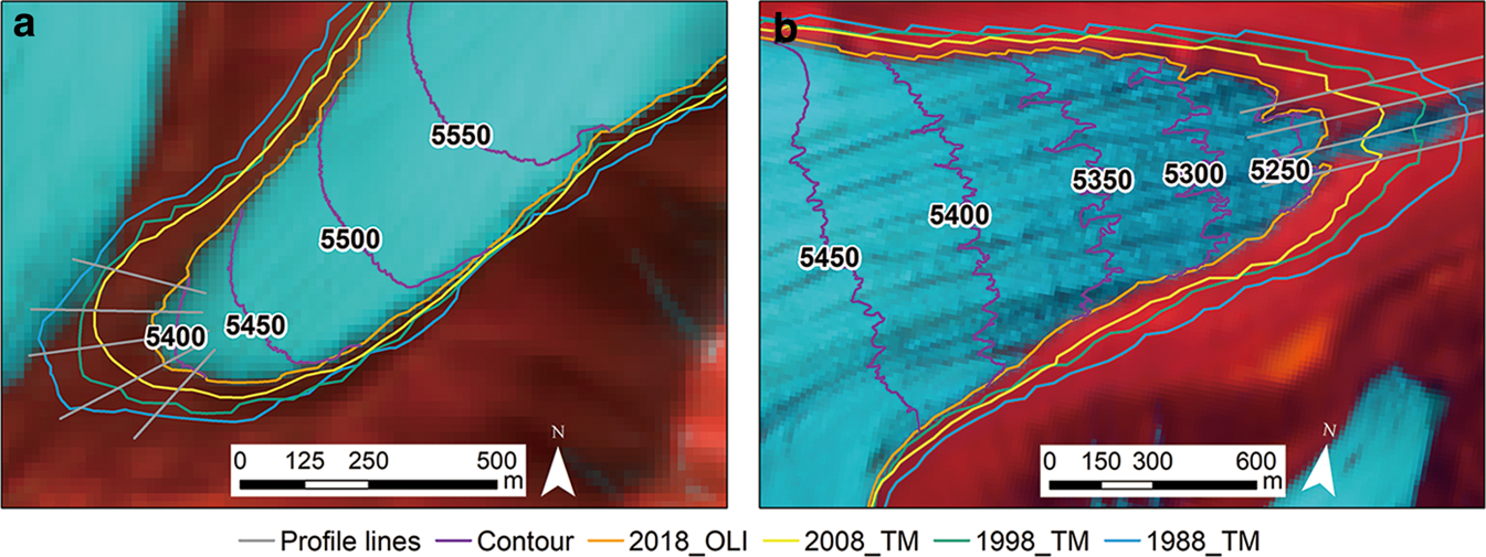
Fig. 6. Borders of the tongue of XDKMD Glacier (a) and GLJM Glacier (b) from 1988, 1998, 2008 and 2018 were outlined based on the Landsat TM/OLI data.
3.4.2 UAV
The super-high resolutions of the UAV products make it easier and more accurate for us to manually outline the glacier boundaries. In most cases, we directly outlined the glacier boundary based on the orthomosaic. For some parts with snow cover, we employed the hillshade assist for recognizing the boundary. Similarly, we calculated the average length of several profile lines we drew at the terminus as the average retreat length of the glacier.
3.5 Error estimation
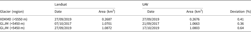
High-resolution UAV images were applied to quantify the accuracy of the glacier delineation from Landsat imagery. Our study area is clean and small without the need for further co-registration; so the main error is the uncertainty related to the glacier delineation. This uncertainty depends on the image resolution (Hall and others, Reference Hall, Bayr, Schöner, Bindschadler and Chien2003). Thus, we confirm the magnitude of this error based on the comparison of outlines from UAV and Landsat (Table 3).
Table 3. Comparison of the outlines from UAV and Landsat
We use the elevation change in the off-glacier area to assess the error of co-registration between repeated UAV surveys. The influence of glacier movement to its surrounding terrain exists but can be disregarded over a relatively short term. Thus, the elevation difference in the off-glacier area should be near zero. We have outlined several off-glacier zones and extracted their elevation difference to quantify the accuracy of the co-registration.
4. Results
4.1 Glacier changes over the last 30 years observed from Landsat imagery
The most direct evidence of the shrinkage of the two glaciers is the change in their termini. The terminus of XDKMD Glacier was connected to its main glacier at one time, but it was found to have separated from the main glacier during the field observation at the end of 2007 (Qiao, Reference Qiao2010). Moreover, the GLJM Glacier surface became broken due to the formation of supra-glacial drainage (which is shown in Section 4.2). We outlined the boundaries of XDKMD Glacier and GLJM Glacier based on the Landsat imagery and discovered that both glaciers retreated rapidly over the past 30 years. The glacier terminus decreased 176 m from 1988 to 2018 at a rate of 5.9 m a−1, and the change rate in the third decade (third bar in Fig. 7a) was the fastest, which was also observed with GLJM Glacier. However, it seems that GLJM Glacier retreated more dramatically; the comparison of the outlines from different years (Fig. 6) reveals that the terminus was scoured out into multiple branches by meltwater. According to our statistics, GLJM Glacier's terminus length decreased ~415 m since 1988, which was a reduction of 13.8 m a−1, twice the decrease in that of XDKMD Glacier.
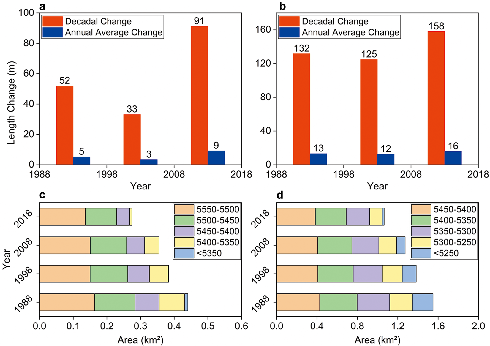
Fig. 7. Changes in the termini over the last 30 years. (a) and (b) show the changes in the lengths of XDKMD Glacier and GLJM Glacier, respectively; (c) and (d) show the changes in area of XDKMD Glacier and GLJM Glacier, respectively.
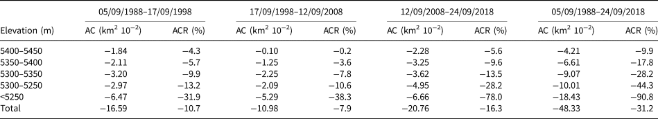
To assess glacier changes more accurately in each part, we divided the ablation zone into several elevation intervals based on the high-resolution DEM. As shown in Figure 7, the terminal part is always the region where ablation is strongest. For example, the region below 5350 m a.s.l. on XDKMD Glacier disappeared in 2008 (blue block in Fig. 7c), and after that, the region between 5400 and 5350 m (yellow block) was drastically reduced from 2008 to 2018, and its area shrunk ~0.036 km2, with an area change rate of 84.4% (Table 4). In addition, the terminal part of GLJM Glacier (blue block in Fig. 7d) decreased by ~0.184 km2 over the entire period, with an area change rate of 90.8%. While the region from 5400 to 5450 m decreased by only ~0.042 km2, with an area change rate of 9.9% (Table 5).
Table 4. XDKMD Glacier area change (AC) and area change rate (ACR) at different elevation intervals
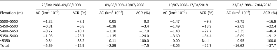
Table 5. GLJM Glacier area change (AC) and area change rate (ACR) at different elevation intervals
4.2 Glacier changes in recent years observed from UAV imagery
The high-resolution images obtained from the UAV are a significant improvement over the data obtained from satellite remote sensing. Based on the difference in the products generated from four aerial surveys, we calculated the terminal change and surface elevation change of XDKMD Glacier and GLJM Glacier in each corresponding period.
4.2.1 XDKMD glacier
The results show that XDKMD Glacier retreated with an average distance reduction of ~3.9 m; decreased in terminal area of 2.3%, and area reduction of 0.0032 km2 in the region below 5500 m a.s.l. The western side of XDKMD Glacier exhibited stronger shrinkage than the eastern side of XDKMD Glacier during the ablation season. From Figure 8, the change in XDKMD Glacier from 20th July to 27th September can be seen in more detail.
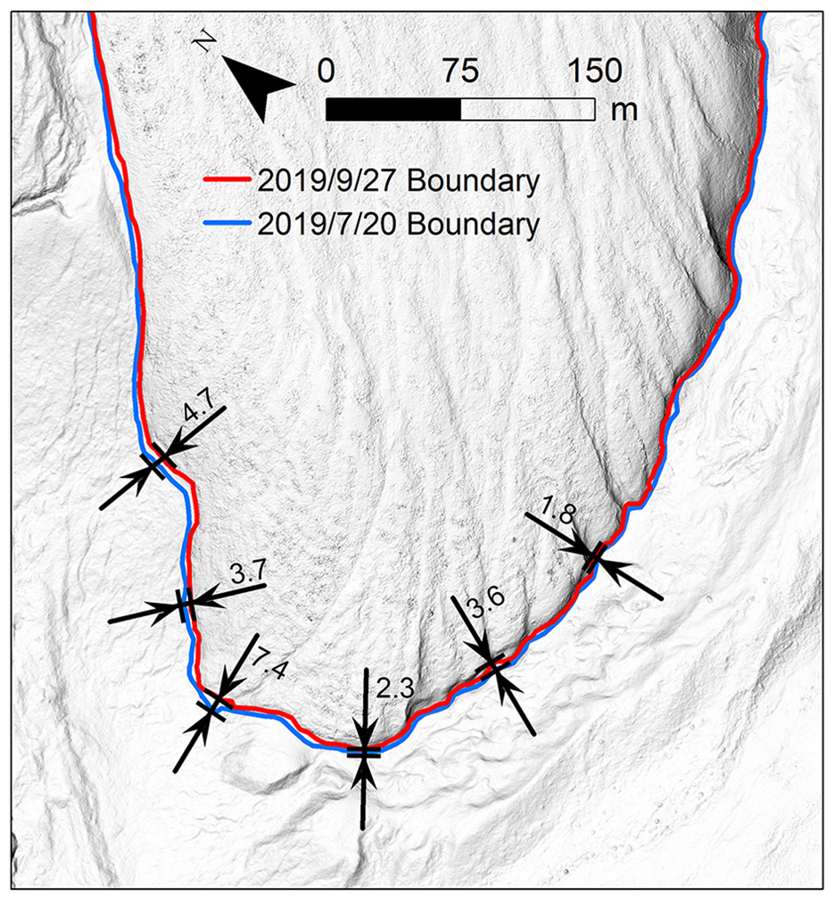
Fig. 8. Terminal length changes (meters) of XDKMD Glacier derived from two UAV surveys. The basemap is a hillshade generated from the DEM in 27/09/2019.
Based on the high-resolution DEM, the surface elevation changes in the glacier terminus during the ablation season can be measured accurately. As shown in Figure 9, most regions in the ablation zone thinned ~2–3 m. The marginal section of the glacier terminus had a relatively large elevation change, with a minimum ice loss of ~3 m and a maximum ice loss of ~8.5 m, which may be attributed to glacier retreat. Notably, several supra-glacial drainage areas appeared on the terminus.
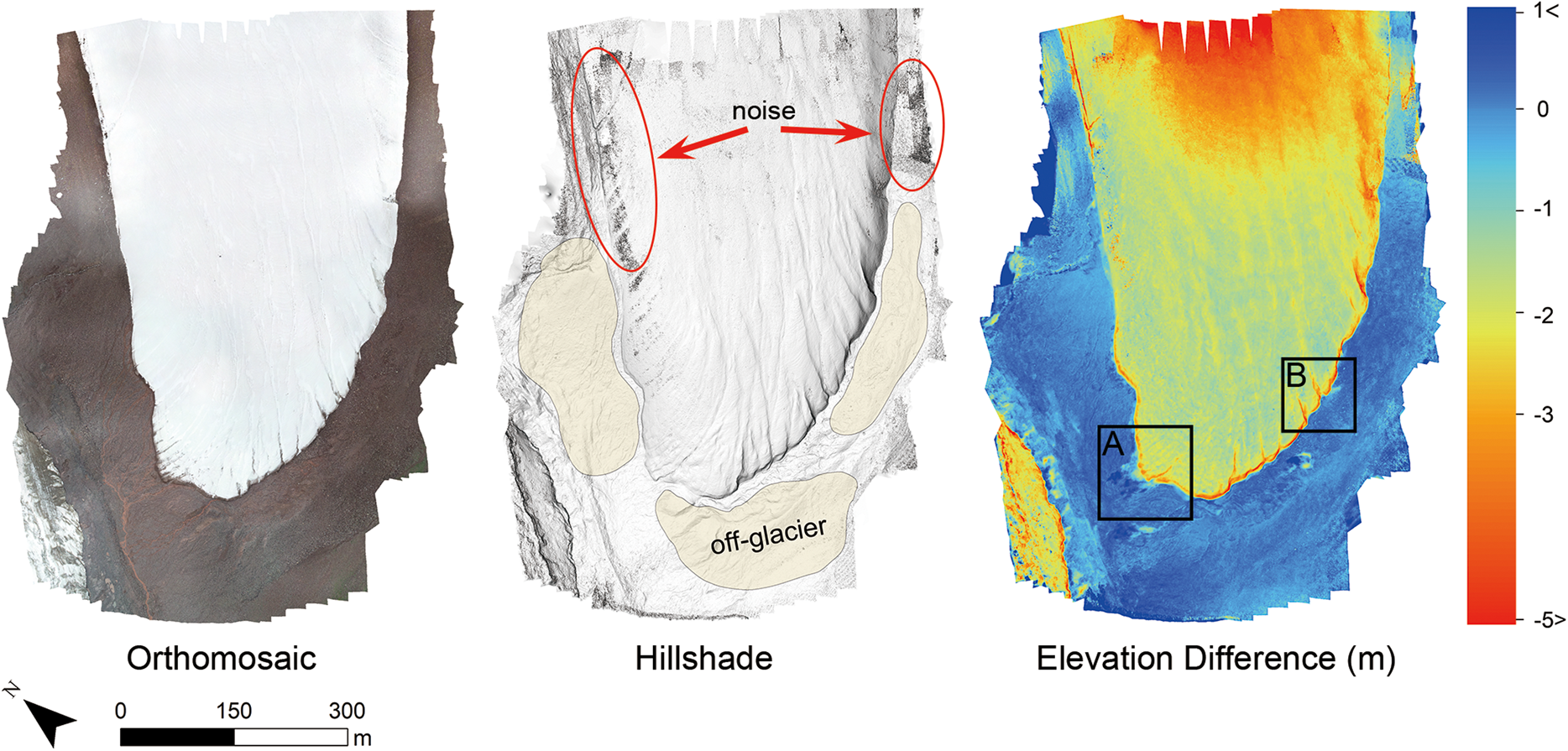
Fig. 9. Orthomosaic in 20/07/2019. Hillshade was generated from the DEM in 20/07/2019 (beige blocks are off-glacier area that outlined for accuracy validation). Elevation difference was detected from the DEMs in 27/09/2019 and 20/07/2019.
4.2.2 GLJM Glacier
Different from XDKMD Glacier, deep crevasses, which are clearly shown in Figure 10, formed on the surface of GLJM Glacier due to years of erosion by meltwater. These crevasses continue to widen and deepen as meltwater conduits have already formed. The area below 5400 m a.s.l. was reduced by 0.0529 km2 during the last 2 years with an area change rate of 3.6% per year, and there is no doubt that the glacier terminus was the area where ablation was strongest, with an average retreat length of 49.7 m from 2017 to 2019.
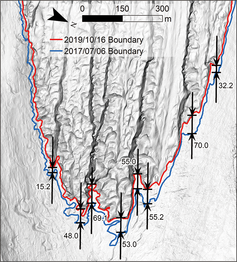
Fig. 10. Terminal length changes (meters) of GLJM Glacier derived from two UAV surveys. The basemap is a hillshade generated from the DEM in 16/10/2019.
As shown in Figure 11, the surface elevation of GLJM Glacier changed dramatically over the last 2 years, especially on the east side of the glacier margin (exact direction of sunlight in the morning) where the elevation changes even more than 16 m due to glacier shrinkage. Four main meltwater conduits on the top of the glacier separated the terminus into five branches, which will promote the formation of a fractured glacier and ice collapse and exacerbate glacier melting (Fig. 11f). Similar to the dirty surface (Fig. 11b), the meltwater remains that we captured near the conduits in July 2017 have a lower albedo than the surrounding area, which indicates intense glacier melting. Most regions of the terminus of GLJM Glacier show an ice loss of ~5–12 m (Fig. 11a).
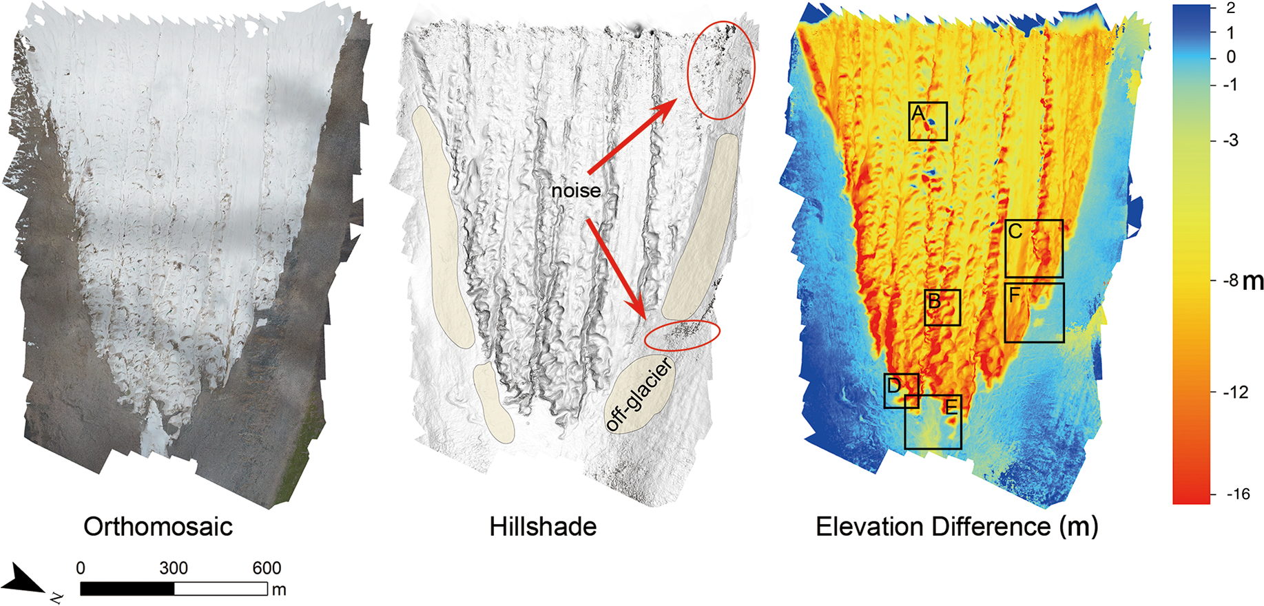
Fig. 11. Orthomosaic in 06/07/2017. Hillshade was generated from the DEM in 06/07/2017 (beige blocks are off-glacier area that outlined for accuracy validation). Elevation difference was detected from the DEMs in 06/07/2017 and 16/10/2019.
5. Discussion
5.1 Accuracy of the results
We determined the horizontal error of our results (length, area change) is about 3 pixels (0.27 m) by comparing stone positions in overlapping orthomosaics. Normally, the vertical error is larger than the horizontal error, especially in places with significant topographic changes. Thus, we selected several off-glacier zones to extract the elevation difference for quantifying the vertical accuracy of the results (elevation change). From the two histograms in Figure 12, we can see that the deviations in the off-glacier region in XDKMD Glacier and GLJM Glacier are controlled at ±0.5 m and ±1 m, respectively. Ideally, the elevation change in off-glacier area is zero. We interpreted such deviation as the following two causes: image quality (include overlap), error of reference products.

The accuracy of our results is mainly influenced by image quality. Image acquirement in a high mountain glacier is challenging due to the hostile environment, such as unpredictable weather. We often encountered several weather events during one survey, and the images that we captured in different light conditions caused shadow stripes, as shown in the orthomosaic in Figure 11. Different light conditions may cause noise on point cloud, which can be seen clearly in the hillshade (Figs 9 and 11). The formation of such noise on point cloud is because the original images have different levels of shade which confused the matching algorithm. Additionally, the number of images that cover the edge of the survey zone is insufficient, and the point cloud that is generated from the images is relative sparse; thus, the edge of the products has low accuracy (Fig. 9).
The limitation of our research is lack of enough and well-distributed GCPs to improve and validate the accuracy of our final products. Thus, the absolute accuracy of the final products, which is poor, may influence other co-registered products. Additionally, the features we marked as MTPs are erratic boulders close to glacier. These erratic boulders around glacier may be influenced by glacier movement and topographic changes. And this may explain the reason that the vertical error of 2 years' change of GLJM glacier is slightly larger than that of seasonal change of XDKMD glacier. However, the settlement of GCPs in a high mountain glacier is a very difficult work. The sub-optimal method that quantifies the glacier change in a relative way has been proved feasible by previous research (Benoit and others, Reference Benoit2019).
5.2 Glacier surface characteristics
Comparing the ablation modes of the two glaciers, some commonalities exist. Although storage meltwater has not been detected on XDKMD Glacier, the beginning of a supra-glacial drainage area has developed, as shown in Figure 9. For GLJM Glacier, supra-glacial drainage areas have formed. Under the influence of these meltwater conduits, the terminus of the glacier was separated into multiple branches, which further facilitated ice collapse and fragmentation. In addition, these conduits are enlarged continuously and will lead to faster glacier recession. Despite this phenomenon, the formation of seracs in GLJM Glacier is not likely due to the fast recession speed.
Figure 13a shows the part with the longest retreating distance, which is also the direction that was once connected to the main glacier. As the terrain of this place is relatively lower, part of the glacial meltwater flows from here and joins the river. Several crevasses at the glacier terminus formed where the glacial meltwater flows occurred (Figs 13a, b). These crevasses have stronger ice loss than other nearby areas. With the continuous meltwater scouring along the existing trajectory, meltwater conduits may form on top of XDKMD Glacier, which would certainly accelerate glacier melting. More notably, the crevasses are dirtier than the surrounding area, which may explain why these crevasses melt faster than other areas.
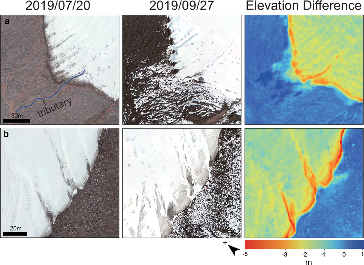
Fig. 13. Detailed changes in selected area in XDKMD Glacier (the location of these images is shown in Fig. 9). The left column shows the orthomosaic in 20/07/2019. The middle column shows the orthomosaic in 27/09/2019. The right column shows the elevation difference.
There are many signs that indicate the rapid melting of GLJM Glacier, such as the undulating surface, storage water, dirty surface and ice collapse. The surface of the GLJM Glacier is undulating due to the heterogeneous surface ablation rate and erosion of meltwater. A positive balance is observed in several places on the terminal of GLJM Glacier, as shown in Figure 14a, the area encircled by a solid black line shows an increase in elevation of ~1–4 m. The arrow in Figure 14a points to a meltwater conduit. Apparently, the conduit has moved and deformed during the two UAV surveys. This movement is also displayed in Figure 14b.
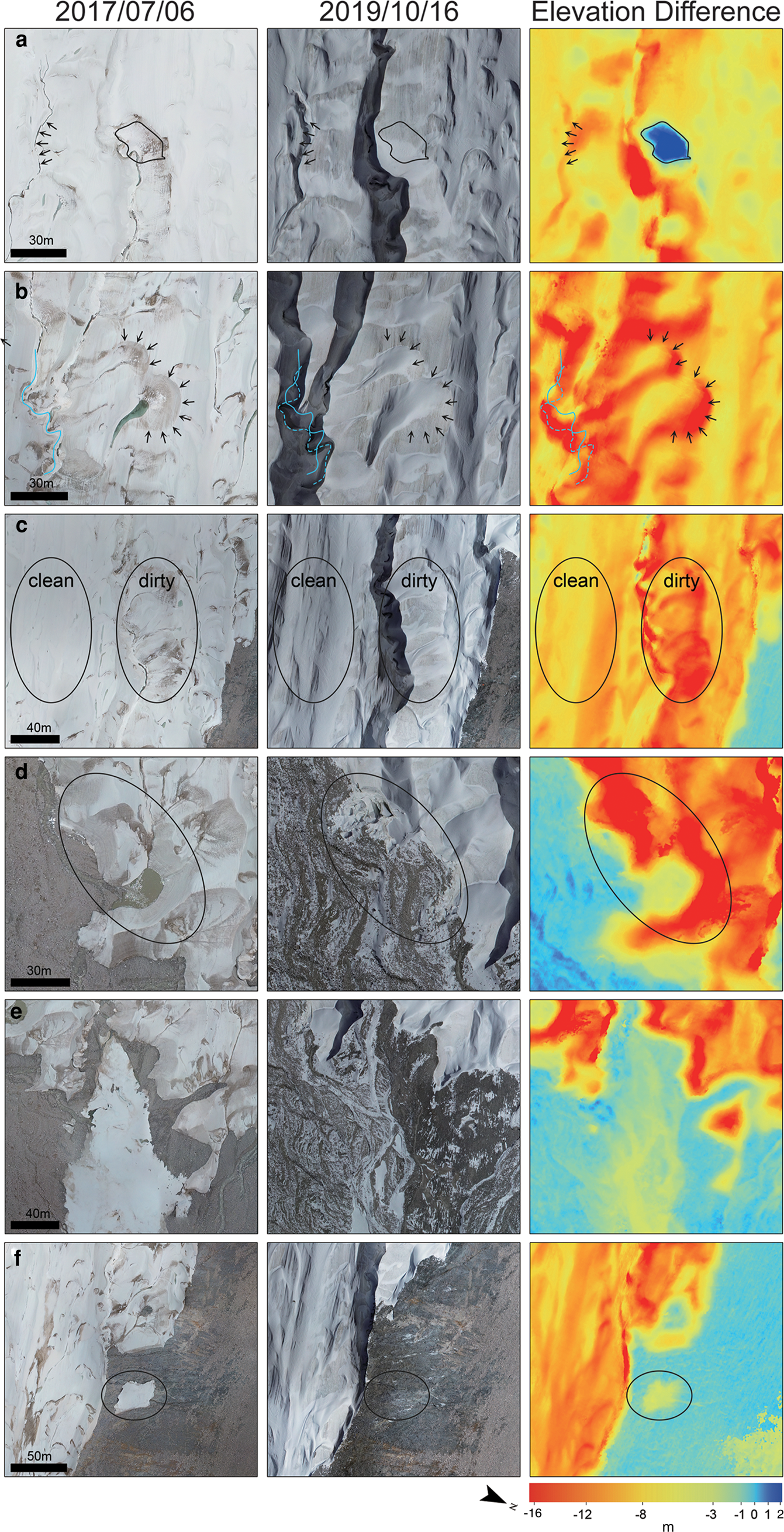
Fig. 14. Detailed change in selected area of GLJM Glacier (the location of these images is shown in Fig. 11). The left column shows the orthomosaic in 06/07/2017. The middle column shows the orthomosaic in 16/10/2019. The right column shows the elevation difference.
Figure 14b shows an example of the existence of storage water on the surface of GLJM Glacier at the beginning of the ablation season. The water storage area has a lower albedo than the surrounding ice surface, resulting in faster ablation and unique erosional features.
We manually classified Figure 14c into two areas: the clean area and the relative dirty area. The dirty area, which is closer to the meltwater conduit, has a larger mass loss than the clean area. We explained such phenomenon as the cause of enrichment of insoluble particles. Water from melting ice and snow flows down conduits, leaving insoluble particles to adhere to the glacier surface near these conduits. These particles reduce the albedo of glacier surface and further accelerate the melting process of glacier.
Figure 14d shows an ice collapse in the lateral branch of GLJM glacier, which may be caused by sub-glacial drainage or water erosion. This might indicate drastic ablation of GLJM glacier. Figure 15 provides another angle of this ice collapse in a 3D mode.
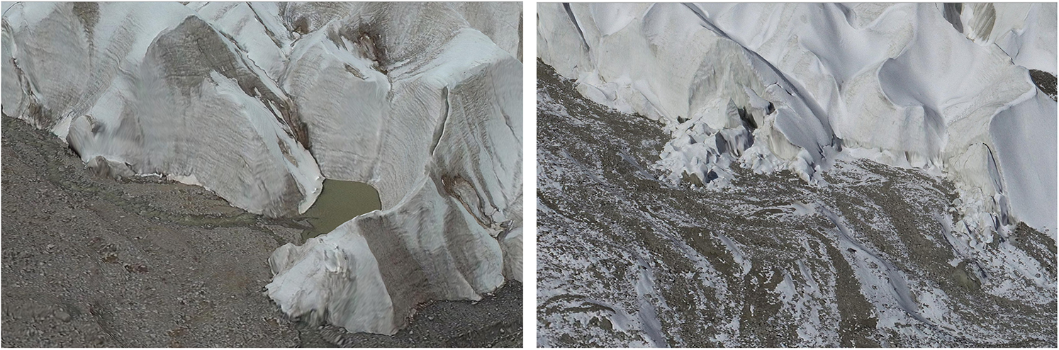
Fig. 15. Ice collapse in the lateral branch in 2017 (left) and 2019 (right) in a 3D model view.
Figure 14e shows the river at the terminus of GLJM Glacier. The river water volume is very large in July due to the strongest glacier melting. Meanwhile, the thick river ice begins to melt (Fig. 2b). Until the end of September, when the glacier begins to enter the accumulation season, the river water volume decreases and the river ice melts completely. Therefore, there is a slight elevation change at the terminal river during each ablation season.
Figure 14f shows the fractured part of the glacier, which is a sign of the drastic ablation. The water erosion and attachment of the light absorbing impurities result in heterogeneous ablation mode, which may lead to the formation of independent ice bodies. The fraction melts quickly which reveals that the formation of seracs in GLJM Glacier is impossible (e.g. Fig. 16).
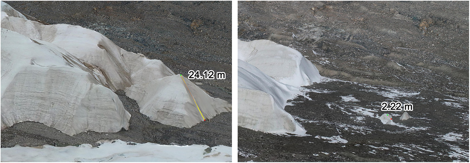
Fig. 16. Part of a fractured glacier in the terminus in 2017 (left) and 2019 (right) in a 3D model view.
5.3 Glacier response to climate change
Glacier change is one of the key indicators of climate change, and some works have shown that glaciers located at high altitudes, especially for those with small size, are more sensitive to climate change (e.g. Diolaiuti and others, Reference Diolaiuti, Bocchiola, D'agata and Smiraglia2012; D'Agata and others, Reference D'Agata, Bocchiola, Maragno, Smiraglia and Diolaiuti2014). Therefore, the rapid change in glaciers in our study area is likely indicative of local climatic fluctuations. To further understand why these glaciers changed so dramatically, we analyzed the data recorded by the automatic metrological station near the two glaciers.
A glacier's response to climate change has a time lag due to the downstream mass transport and deformation of the glacier (Pattyn, Reference Pattyn2002), Wang and Zhang (Reference Wang and Zhang1992) determined there was a time lag of about 12 years for glacier response to climate change in the Northern Hemisphere. Considering glaciers with small size are more sensitive to climate change, we assume there exist a decade lag in this paper and extend the beginning of the time series of the temperature and precipitation graphs to 1978. By an analysis of the temperature trends, we discovered that the annual mean temperature significantly changed in our study area since 1978 and both stations' records show very large rates of increase (Fig. 17). The annual rates of mean temperature increase at Tuotuohe station and Nagqu station are 0.65°C a−1 (R 2 = 0.51) and 0.60°C a−1 (R 2 = 0.69), much higher than the global warming magnitude 0.15–0.20°C a−1. The annual precipitation shows a large fluctuation, which cannot be well fitted. Thus, we calculated the decadal average precipitation and temperature to make a better trend analysis, and a better comparison with the glacier changes in the corresponding period as well.
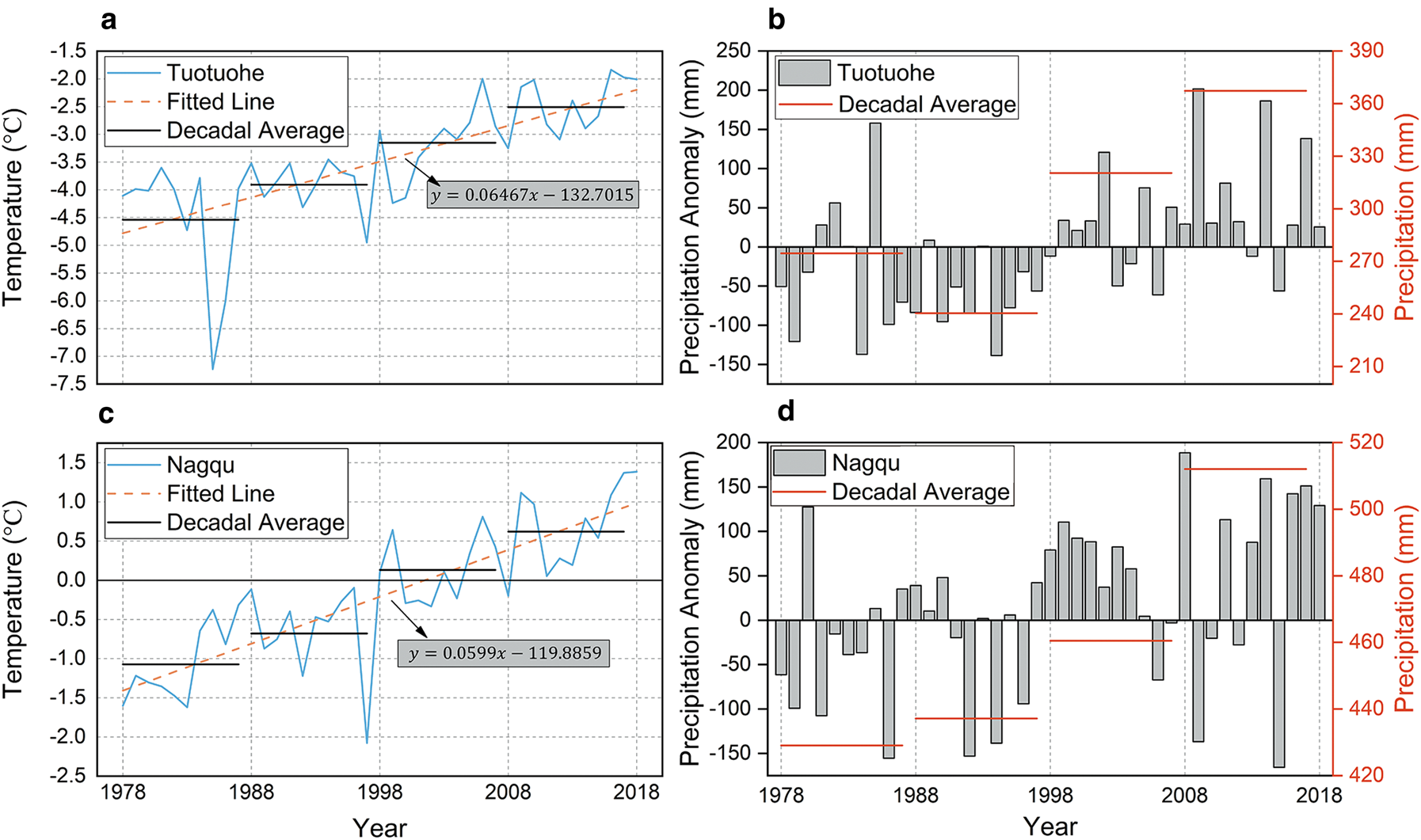
Fig. 17. Temperature and precipitation measured at Tuotuohe station and Nagqu station from 1978 to 2018.
Compared with the first decade (1978–1988), the decadal average temperature in the second decade (1988–1998) rose by 0.64°C in Tuotuohe station and 0.39°C in Nagqu station, while the decadal average precipitation slightly increased (1.89% in Nagqu station) or even decreased (−12.45% in Tuotuohe station). This may explain why there was a reduced glacier area change rate in the following 10 years. Additionally, the sudden temperature dropped around 1997, which also reported by Ke and others (Reference Ke, Ding, Li and Qiu2017), may also contributed to this reduced change rate. The largest warming magnitude (0.76°C in Tuotuohe station; 0.81°C in Nagqu station) was between the second decade and the third decade (1998–2008). And at the meantime, decadal average precipitation had a comparable increase (33.29% in Tuotuohe station; 5.34% in Nagqu station), which should have slowed down glacier melting. However, the melting rate of these two glaciers did not decrease in the fourth decade (2008–2018), but reached its highest level in the past three decades with area change rate of 22.7% in XDKMD and 16.3% in GLJM glacier. Kang (Reference Kang1996) indicated that precipitation needs to increase by at least 40% to offset the effect of a one-degree rise in temperature on the glacier. Similarly, our analysis of glacier response to climate change might imply that slight increase in precipitation in our small study area made a limited contribution to glacier change, while rise in temperature has a greater impact on glacier.
6. Conclusion
In this study, we conducted four UAV surveys, for the first time, on two debris-free glaciers on the central TP. By co-registration of these UAV products, we quantified the termini, area and elevation change of the two glaciers in a short term, and further discussed surface characteristics based on the high-resolution products. Additionally, we utilized eight Landsat scenes to measure the termini and area change of the two glaciers in the past 30 years. From the study, we draw the following conclusions.
During the last 30 years, the terminus of XDKMD Glacier retreated 176 m, with an area decrease of 0.17 km2 (altitude below 5550 m a.s.l.), and the terminus retreat and area shrinkage of GLJM Glacier were 415 m and 0.18 km2, respectively (altitude below 5450 m a.s.l.). The fastest decade of glacier melting occurred from 2008 to 2018. During this time, XDKMD Glacier retreated 9 m a−1 and had a terminal area shrinkage of 2.3% per year and GLJM Glacier retreated 16 m a−1 and had a terminal area shrinkage of 1.6% per year. During the ablation season, XDKMD Glacier retreated by 3.9 m; the terminal area shrank by 2.3%; and the surface elevation of most areas changed by 2–3 m. From 2017–2019, GLJM Glacier retreated by 24.9 m a−1; the terminal area shrank by 3.6% per year; and the surface elevation of most areas changed by 8–12 m.
Acknowledgements
This work was funded by the National Natural Science Foundation of China (41671071, 41730751 and 41771040) and the Open Foundation of State Key Laboratory of Cryospheric Sciences (SKLCS-OP-2019-04). We thank the Tanggula Cryosphere and Environment Observation Station for field assistance.


 Open access