Introduction

The ice shelves fringing Antarctica provide an important interface between the grounded ice sheet and the oceans (Reference Vaughan and ArthernVaughan and Arthern, 2007). Increased ocean temperature (and hence basal melting) has been implicated in the thinning of Pine Island Glacier, West Antarctica, and the collapse of parts of the Larsen Ice Shelf, Antarctic Peninsula (Reference Shepherd, Wingham, Payne and SkvarcaShepherd and others, 2003, Reference Shepherd, Wingham and Rignot2004). Numerical studies of simplified ice-shelf cavities show the strong effect that cavity shape has on basal melt rates (Reference Holland, Jenkins and HollandHolland and others, 2008). As such, ice draft and bathymetry are important parameters for numerical models which simulate sub-ice circulation patterns and melt/freeze rates (e.g. Reference Nøst and FoldvikNøst and Foldvik, 1994).

The Amery Ice Shelf (AIS) is the major embayed ice shelf of East Antarctica (Fig. 1) and drains ∼16% of the grounded East Antarctic ice sheet through Lambert Glacier and other tributary glaciers (Reference AllisonAllison, 1979). The geometry of the cavity beneath the AIS is thought to have a strong influence on the thermohaline circulation (Reference Williams, Jenkins, Determann, Jacobs and WeissWilliams and others, 1998) and is important for sediment studies (e.g. Reference Hemer and HarrisHemer and Harris, 2003), biological studies (e.g. Reference Riddle, Craven, Goldsworthy and CarseyRiddle and others, 2007) and palaeoclimate studies of past grounding-line positions (e.g. Reference O’Brien, Goodwin, Forsberg, Cooper and WhiteheadO’Brien and others, 2007).

Fig. 1. The location of Amery Ice Shelf and Prydz Bay in East Antarctica (black box in inset). (a) The bathymetry data used in the interpolation: black dots show the location of the seismic data, the grey curve shows the ice-draft data taken at the grounding line and the dashed grey curve in the southern region of the AIS is the prescribed channel centre line. (b) The locations of the 11 GPS observation sites and major features of the Amery Ice Shelf region.

The AIS cavity geometry and grounding line has been redefined a number of times since early modelling studies by Reference Williams, Jenkins, Determann, Jacobs and WeissWilliams and others (1998). Reference FrickerFricker and others (2002) estimated that the southern limit of the grounding line was 240 km further south than prior estimates (Reference Budd, Corry and JackaBudd and others, 1982), and most recently L. Giovanna and others (personal communication from N. Young, 2007) used observations from moderate-resolution imaging spectroradiometer (MODIS) and synthetic aperture radar (SAR) studies to infer grounding-line positions from the break in the surface slope topography (shown as the solid black curve in Fig. 1b).

Available bathymetry data beneath the AIS are restricted to regions that are easily accessed in the field and do not extend south of 71.6° S on the AIS, which is shown here to have a southern limit at 73.6° S (see Fig. 1a for data locations). As a consequence, the shape of the AIS cavity south of 71.6° S is largely unknown. Future seismic studies of the southern region are uncertain due to the location (the area has many crevasses and is riddled with summer surface melt features) and challenging logistics (the area is >600 km from Davis, the nearest base station), although such surveys provide the most direct and accurate measurements of ice draft and water-column thickness. Any opportunity to make measurements in this region is probably many years away under current field-programme logistical support plans of the Australian Antarctic Division. These reasons necessitate the use of an alternative method to achieve a bathymetry that is as accurate as possible.

Here, we refine a method, first used by Reference Hemer, Hunter and ColemanHemer and others (2006), to determine the general cavity shape beneath the AIS. Reference Hemer, Hunter and ColemanHemer and others (2006) showed that the water-column thickness (WCT), which is the difference in depth between the ice-shelf draft and bathymetry, in the unknown areas beneath an ice shelf can be inferred with the aid of a tidal model. We have improved the method of Hemer and others by including the most up-to-date bathymetry and ice-draft data and modelling the tides at a much higher resolution. The original sparse bathymetry data have been supplemented with data from new seismic surveys, direct observations through boreholes in the floating ice shelf and ice-draft radar data, taken at the grounding line. The updated grounding-line position provided by N. Young (personal communication, 2007) is also used to provide the most up-to-date map of the AIS cavity geometry.

We use a high-resolution hydrodynamic tidal model (MOG2D) to produce tidal predictions for ten different estimates of the WCT, with the values for WCT chosen to be within what we believe to be plausible ranges. These tidal predictions are then compared with GPS (global positioning system) observations of the tidal amplitude and phase measured at various locations on the AIS (see Fig. 1b for GPS locations). The most appropriate WCT corresponds to the smallest difference of the complex sum between the observed and predicted harmonics for the four main tidal constituents (K1, O1, S2, M2), which represent ∼80% of the total tidal variance in this region.

This paper presents a refined cavity geometry for the AIS. Bathymetry data from seismic surveys and direct observations are supplemented here with ice-draft data taken at the grounding line. The grounding-line position for the AIS was taken as the point at which WCT goes to zero. All the available bathymetry data are combined and merged with bathymetry data in Prydz Bay to produce a final continuous bathymetry map beneath the AIS on a 2 km × 2 km grid.

AIS Geometry Data

Ice draft

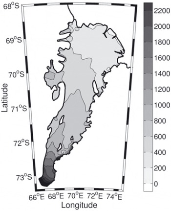
Surface elevations and ice thicknesses have been measured over much of the area using satellite radar altimeter and radio-echo sounding. The elevation and thickness estimates of Reference Fricker, Hyland, Coleman and YoungFricker and others (2000, Reference Fricker2002) are used here. The ice drafts were found by subtracting the elevation from the ice-thickness data. The ice-draft data were then resampled onto a 2 km grid using nearest-neighbour interpolation, which also removed gaps in the dataset. This resulted in a continuous ice-draft map for the entire area of the AIS, which is shown in Figure 2.

Fig. 2. Ice draft of the AIS showing 200 m contour intervals.

The uncertainty in the observations was estimated by comparing the gridded ice draft with independent radio-echo sounding measurements of ice thickness collected as part of the Prince Charles Mountains Expedition of Germany and Australia (PCMEGA) campaign during the 2002/03 Antarctic summer. We find that the PCMEGA data, which are only available for the southernmost region of the AIS, are ∼3% thicker than the gridded ice-draft data. This is ∼75 m at the deepest part of the ice shelf which is ∼2500 m below mean sea level at its southern extremity. This error in the earlier gridded ice-draft data is probably due to underestimating the ice density in regions of higher ablation, which is typically where the ice shelf is thickest, as in the southern region of the AIS (personal communication from H. Fricker, 2007). We have found that the southernmost grounding line is deeper than BEDMAP estimates by ∼450 m (Reference Lythe and VaughanLythe and others, 2000) and is one of the deepest grounding lines of any ice shelf.

Gridding method

Ice-draft data at the grounding line were extremely useful in the interpolation of the bathymetry. The grounding line is where the base of the ice shelf coincides with the sea floor. It is important to include these data in the interpolation because they help constrain the shape of the AIS cavity. The ice-draft data were interpolated using nearest-neighbour interpolation to each known grounding-line location, which is made up of 1317 points. The grounding-line locations are shown as the grey curve in Figure 1a. Note that this is made up of individual inferences of the grounding-line position. The combined dataset, involving both bathymetry and grounding-line locations, contained 1436 data points compared with only 72 in the work of Reference Hemer, Hunter and ColemanHemer and others (2006).

The 2 km × 2 km grid covered the Prydz Bay depression from 66° E to 79° E and from the southernmost extension of the AIS at 73.6° S to the shelf break at ∼66° S. This created 120 291 (397 × 303) interpolation sites. All available sub-ice-shelf bed-elevation data and Prydz Bay bathymetry data (a combination of ship-track measurements supplied by the Australian Antarctic Division Data Centre and the General Bathymetric Chart of the Oceans (GEBCO) 1 min bathymetric data of IOC and others, 2003) were interpolated onto the model grid using a Universal Transverse Mercator projection (WGS84). The bathymetry data were gridded using a kriging technique with an isotropic variogram which was linear within the correlation radius and zero outside. The correlation radius was chosen to be 6 km, based on the average data density in the northern region of the AIS. The standard error introduced by the kriging technique can be calculated by comparing the elevation from the interpolated grid with the observations at each location. This yields a standard error in the bathymetry interpolation, excluding the ice-draft data taken at the grounding line, of about ±6 m. The standard error in the bathymetry interpolation at the grounding line is about ±2 m. The lower standard error at the grounding line is due to the higher data density in this region.

A range of ten possible choices of bathymetry was created by incorporating synthetic data into the interpolation from along the prescribed channel centre line, which is shown as the dashed grey curve in Figure 1a. Each of the ten choices of bathymetry used a single prescribed value of WCT that was added to the value of the overlying ice draft along the channel centre line. The values added to the ice draft along the channel centre line were 170, 470, 770, 1070, 1370, 1670, 1970, 2270, 2570 and 2870 m. The effect can be seen in Figure 3, which shows the range of south–north and east–west profiles created, following the two transects shown in the inset of Figure 3a. The WCT was constrained to a minimum of 10 m. The tidal model requires just the WCT, which was calculated from the difference between the bathymetry and the ice draft.

Fig. 3. Vertical sections along transects (a) south–north and (b) east–west as shown in the inset. Ten possible choices of bathymetry are shown. The best estimate is the black dashed curve. Each bathymetric choice was created by varying the thickness of the water column below the ice shelf along the dashed grey curve shown in Figure 1a. The intersection point of the two transects is shown in (a) and (b) by a vertical black line.

Tide Model

Each choice of WCT was tested in MOG2D, which is a barotropic time-stepping and non-linear two-dimensional (vertically averaged) gravity-wave model, based on that of Reference Lynch and GrayLynch and Gray (1979). In regions where there is an ice-shelf cavity, the WCT (rather than the depth of the sea floor) is the appropriate ‘water depth’ to use in the model. MOG2D computes the sea-surface height and mean currents due to wind and tidal forcing by solving the shallow-water momentum and continuity equations on a finite-element mesh. This spatial discretization allows the resolution to be coarser in the deep ocean and finer in coastal regions and those with strong topographic gradients, enabling good simulation of gravity waves. The spatial resolution is based on the WCT, its gradient and the wavelength of the gravity waves (Reference Le Provost and VincentLe Provost and Vincent, 1986).

The model domain covers the southern area of the Indian Ocean with a grid ranging in size from a few kilometres on the continental shelf, including the AIS region, to 100 km in the deep ocean. Details of the finite-element mesh are given by Reference Maraldi, Galton-Fenzi, Lyard, Testut and ColemanMaraldi and others (2007). By calculating tides for a range of plausible WCTs in unsampled areas in the southern AIS, we can produce a map of WCT values that provides the optimum agreement between modelled and measured (GPS) tides.

The coefficient used for tidal bottom friction parameterization was taken to be 0.0025 and, following other studies, was doubled for the area covered by the ice shelf (e.g. Reference MacAyealMacAyeal, 1984). Dissipation due to ice-shelf flexure caused by the tidal motion is not accounted for at the grounding line; the ice shelf is considered to be freely floating. The open boundaries are forced using the harmonic constants (amplitude and phase) obtained from the FES2004 global barotropic solution (Reference Lyard, Lefevre, Letellier and FrancisLyard and others, 2006). Three semi-diurnal (M₂, S₂, N₂) and three diurnal (K₁, O₁, P₁) tidal constituents were modelled. The model was run for 40 days, including a 3 day spin-up period. The harmonic analysis was performed on the last 30 days so that each of the constituents was well resolved.

Data Analysis

GPS data from 11 records were used to validate the tide model (see Table 1). Tidal amplitude and phase for the four main constituents were found for each GPS record. GPS data from sites 1, 2, 3, 5 and 11 (Fig.1b) have records long enough that tidal analysis may resolve M₂ from S₂ and K₁ from O₁ (i.e. >15 days). Records shorter than this were analysed for M₂ and K₁, where S₂ and O₁ were deduced using amplitude and phase relationships from the longer tidal records from Davis station. The errors in analysing specific constituents from short record lengths (i.e. less than ∼3–4 days) can be large. We combined sites that had short length records and were within 20 km of each other to make longer time series to reduce this error: record 6 is a concatenation of sites 6a, 6b and 6c and record 8 is a concatenation of sites 8a and 8b (Fig. 1b; Table 1). Typical GPS measurement precisions are ∼1–5% of the tidal range, which for the AIS are ∼1–5 cm (Reference KingKing, 2002, Reference King2006; Reference Zhang and AndersenZhang and Andersen, 2006).

Table 1. The complex error, ∊ (cm) for this study (TS) and Reference Hemer, Hunter and ColemanHemer and others (2006) (H06) for GPS sites 1–11. The bottom row is the root-mean-square value calculated over sites 1–10. Site 11 is excluded from the rms calculation as it lies in the ice-shelf flexure zone

For each choice of WCT, the tidal solutions from MOG2D as a time series were compared to the GPS ellipsoidal height data that were measured over the AIS (see the crosses in Fig. 1b for the locations). The sensitivity of the model to changes in the WCT is obtained using the modulus of the complex difference between observations and model predictions (the ‘complex error’), which is calculated as:

(1)

where z = Ae ^{i ϕ} , A and ϕ being the amplitude (cm) and phase, respectively, of each tidal constituent M₂, S₂, K₁ and O₁. The root-mean-square (rms) error was calculated using

(2)

where N is the total number of tidal constituents. The sensitivity of the model to changes in the WCT is shown in Figure 4.

Fig. 4. The sum of the rms complex errors for the four major tides compared with the mean WCT calculated over the AIS, for (a) the sum of records 1–10, (b) records 1–7, (c) records 8–10 and (d) record 11. Note that record 11 lies within the ice-shelf flexure zone, which acts to damp the tidal amplitude, thereby increasing the complex error, and so was not included in (a).

Results and Discussion

A significant minimum can be seen in the rms error for the simulations (Fig. 4). Summing over GPS records 1–10 shows that the smallest rms between the observations and simulations is for a mean WCT of 367m (Fig. 4a), which is ∼35 m deeper than that estimated by Reference Hemer, Hunter and ColemanHemer and others (2006). In this case, the WCT along the prescribed channel centre line was 1370 m, which is ∼750 m deeper than Reference Hemer, Hunter and ColemanHemer and others (2006). Record 11 (Fig. 4d) was excluded from Figure 4a as it lies in the ice-shelf flexure zone, which can act to damp the tidal amplitude. Ice-shelf flexure is a physical process that is not modelled in MOG2D, which is reflected in the larger rms shown in Figure 4d. The records in the adjusted southern region (records 8–11, Fig. 4c and d) show an increase in the rms toward the southern grounding line of the AIS. Records 8–10 (Fig. 4c) are clearly important contributors for the minimum rms seen in Figure 4a. Otherwise, the records to the north of the cavity (Fig. 4b) are essentially flat and do not contribute significantly to the shape of Figure 4a.

Comparison of the rms errors for the optimum WCT (367 m) with the rms errors from Reference Hemer, Hunter and ColemanHemer and others (2006) shows a significant improvement over all the GPS sites (Table 1). This is especially obvious in the southern region of the AIS for sites 9 and 10 where MOG2D shows large improvements in the semi-diurnal (M₂, S₂) and diurnal (K₁, O₁) tides. Note that Reference Maraldi, Galton-Fenzi, Lyard, Testut and ColemanMaraldi and others (2007) have shown that MOG2D with the best-fit WCT profile has also been found to outperform the regional Antarctic models (CATS and CADA (Reference Padman, Fricker, Coleman, Howard and ErofeevaPadman and others, 2002) and global tide models, TPXO (Reference Egbert, Bennett and ForemanEgbert and others, 1994) and FES2004 (Reference Lyard, Lefevre, Letellier and FrancisLyard and others, 2006)). These improvements are therefore due to both the higher resolution of the tide model and the improved ice draft and bathymetry.

Best-fit cavity geometry

We have produced a refined map of the AIS bathymetry. The new bathymetry map (Fig. 5a) was derived using ice-draft data at the grounding line and a prescribed channel centre line which has the advantage of retaining the cross-sectional aspect of the ice-shelf geometry. Sections through the best-fit bathymetry are shown by the dashed black curve in Figure 3. The differences between the bathymetry of Reference Hemer, Hunter and ColemanHemer and others (2006) and this study are shown in Figure 5b. The main differences occur in the area south of 71.5° S. Most of the change seen in the northern part of the AIS can be attributed to the new grounding-line position and the seismic and borehole data. The best fit continues the north–south trend in the bathymetry that can be seen in the northern part of the cavity (Fig. 3a).

Fig. 5. (a) The resulting bathymetry of the AIS and Prydz Bay regions showing 200m contour intervals. (b) Difference between this bathymetry and that of Reference Hemer, Hunter and ColemanHemer and others (2006), the extra area included in this study indicated as spotted dark grey, and the extra area used by Reference Hemer, Hunter and ColemanHemer and others (2006) shown as light grey (i.e. in some regions near the grounding line such as in Beaver Lake).

The total area of the AIS, less any area covered by Budd Ice Rumples, Clemence Massif, Robertson Nunatak and Gillock and Dog Islands, is 58 380 km². This estimate is 5% larger than the area used by Reference Hemer, Hunter and ColemanHemer and others (2006) (the differences between grounding-line positions can be seen in the dotted dark grey and light grey areas of Figure 5b) and 15% larger than suggested by Reference FrickerFricker and others (2002). Most of the difference in area estimates is seen in the southern grounding-line position. This estimate uses an ice-front position from 2001 which is advancing at a rate of ∼1200 m a⁻¹ (Reference Young and HylandYoung and Hyland, 2002). The total area of the AIS at the time of writing is therefore 60 000 km².

Obtaining a realistic description of the cavity shape is especially important for studies of the ocean circulation in the sub-ice-shelf cavity. This circulation can be described thus: When water at or near the surface freezing point (e.g. high-salinity shelf water) descends into the cavity beneath the ice shelf, it can cause melting near the back of the shelf due to the depression of the freezing point with pressure. The subsequent freshened water (ice-shelf water) can rise along the underside of the shelf and possibly refreeze to the base of the ice shelf, forming marine ice (Reference Lewis and PerkinLewis and Perkin, 1986). Any flow of dense marine waters from Prydz Bay (e.g. high-salinity shelf water) is expected to follow the sea-floor contours. The new bathymetry map (Fig. 5a) suggests that the flow of dense marine waters into the cavity could follow the contours to the very southern grounding line. The ice draft at this depth is 1600 m deeper than that used in studies by Reference Williams, Grosfeld, Warner, Gerdes and DetermannWilliams and others (2001); this has major implications for the amount of melting that can occur in this region.

Conclusions

We have refined a technique that was first used by Reference Hemer, Hunter and ColemanHemer and others (2006) to estimate the bathymetry beneath ice shelves in areas where direct observations are not feasible. We have used a high-resolution barotropic tide model together with GPS-derived tidal heights to estimate the shape of the cavity in the southern region beneath the AIS. New data from seismic-reflection studies undertaken in the centre of the AIS and ice-draft values taken at the grounding line have been used in a kriging interpolation to grid a continuous bathymetry at 2 km × 2 km resolution. The higher resolution of the coastline and bathymetry is shown to deliver significant improvements in tidal elevation predictions in the region beneath the AIS (see Table 1). These results will be of interest to a broad range of disciplines, such as remote sensing, numerical modelling, oceanography and glaciology. These data can be accessed at http://aadcmaps.aad.gov.au

This method can be used to determine the WCT beneath other ice shelves and, with the inclusion of ice-draft data, the cavity bathymetry. This technique can use any surface-elevation data which are of sufficient resolution to resolve tides. Sea-surface elevations, derived from satellite altimetry at crossover points, are a prime example, as demonstrated by Reference Fricker and PadmanFricker and Padman (2002). The altimeter data generally allow better spatial coverage of the ice shelves and produce longer time series, making their use with this technique worth investigation.

These results confirm that the AIS cavity allows the oceans to be in contact with ice at the deepest point known for an Antarctic ice shelf; this has interesting consequences both in terms of glaciology and oceanography.