


Introduction
The largest component of ablation of the world’s cryosphere is calving (Reference Van der VeenVan der Veen, 2002), i.e. the mechanical loss of ice from glaciers and ice shelves (Reference Benn, Warren and MottramBenn and others, 2007a). It has been shown that intense calving can lead to abrupt changes in glacial dynamics, enhancing ice flow by reducing the back-stress (Reference Joughin, Abdalati and FahnestockJoughin and others, 2004). The relationship between observed calving rates and water depth follows regional clusters (Reference HaresignHaresign, 2004), indicating the existence of regional differences in the behaviour of calving fronts. A comprehensive review of calving processes and their modelling is given by Reference Benn, Warren and MottramBenn and others (2007a). They propose a classification of calving mechanisms based on their relative importance. The first-order mechanism of calving is fracture propagation caused by longitudinal stresses driven by acceleration of the front. Fracture propagation can be enhanced by the presence of water in crevasses (e.g. Reference WeertmanWeertman, 1973; Reference Van der VeenVan der Veen, 1998; Reference Alley, Dupont, Parizek and AnandakrishnanAlley and others, 2005), either due to surface melt or rainfall. According to Reference Benn, Warren and MottramBenn and others (2007a) this mechanism usually controls the overall calving flux of tidewater glaciers.
Another, generally less efficient calving mechanism, is undercutting of the ice cliff by melting at or below the waterline and the subsequent break-off of ice slabs. Reference Benn, Warren and MottramBenn and others (2007a) classify this as the second-order mechanism. In this context, melt is less important as a mass sink, but is rather a source of force imbalance at the front and thus a trigger for calving (Reference Vieli, Funk and BlatterVieli and others, 2001). Water temperature and circulation control the melt (e.g. Reference Eijpen, Warren and BennEijpen and others, 2003; Reference Motyka, Hunter, Echelmeyer and ConnorMotyka and others, 2003; Reference JenkinsJenkins, 2011) and therefore this calving mechanism. Enhanced submarine melt due to increased water circulation in the vicinity of subglacial outflows is particularly strong, as buoyant fresh water draws in warm sea water (Reference Motyka, Dryer, Amundson, Truffer and FahnestockMotyka and others, 2013). As pointed out by Reference Benn, Warren and MottramBenn and others (2007a), second-order calving may play the major role for tidewater glaciers with low longitudinal strain rates, i.e. where the velocity gradients are not high enough to cause intense fracturing. In such cases the undercutting of the calving front by melting at or below the waterline and the resulting local imbalance of force at the front will cause calving events of a smaller size. The relative importance of this type of calving remains unknown (Reference Otero, Navarro, Martin, Cuadrado and CorcueraOtero and others, 2010) and it is not taken into account in models (Reference Amundson and TrufferAmundson and Truffer, 2010; Reference Nick, Van der Veen, Vieli and BennNick and others, 2010; Reference Otero, Navarro, Martin, Cuadrado and CorcueraOtero and others, 2010), as it was primarily investigated for the case of freshwater calving (e.g. Reference IkenIken, 1977; Reference Kirkbride and WarrenKirkbride and Warren, 1997; Reference HaresignHaresign, 2004; Reference RohlRohl, 2006).
Reference Vieli, Jania and KolondraVieli and others (2002) hypothesized that, for Hansbreen, melt at the waterline is responsible for the mean summer calving rate, whereas major changes in the terminus position are driven by bed topography. They assumed that the calving rate due to melt at the waterline throughout the summer was constant and equal to the notch melting rate. Therefore, they accounted only for calving of the overhanging slabs, while recent work of Reference O’Leary and ChristoffersenO’Leary and Christoffersen (2013) shows that the undercut notch may influence the stress field relatively deep into the glacier, causing the calving rate to increase as much as three times, compared with a vertical ice cliff with no undercut.
There are three main ways to quantitatively model the calving rates: the first links the calving rate to an independent variable, such as water depth or ice front height (e.g. Reference Meier and PostMeier and Post, 1987; Reference Pelto and WarrenPelto and Warren, 1991; Reference Oerlemans, Jania and KolondraOerlemans and others, 2011); the second specifies the terminus position based on the flotation criterion, which is the height above buoyancy at the glacier terminus (e.g. Reference Brown, Meier and PostBrown and others, 1982; Reference SikoniaSikonia, 1982; Reference VenterisVenteris, 1999; Reference Vieli, Jania and KolondraVieli and others, 2002); the third, and most modern (e.g. Reference Amundson and TrufferAmundson and Truffer, 2010; Reference Nick, Van der Veen, Vieli and BennNick and others, 2010; Reference Otero, Navarro, Martin, Cuadrado and CorcueraOtero and others, 2010), resolves the force balance at the front and applies it to compute transverse crevasse depth (Reference NyeNye, 1955, Reference Nye1957), based on the criterion proposed by Reference BennBenn and others (2007b).
Recent studies focus more on the detailed dynamics of the front (e.g. Reference O’Leary and ChristoffersenO’Leary and Christoffersen, 2013) to account for more subtle effects, such as front geometry. Nonetheless, regardless of its importance for regional mass balance, and thus sea-level rise, calving and related dynamic processes are still poorly represented in state-of-the-art ice-sheet models (Reference Benn, Warren and MottramBenn and others, 2007a). One of the reasons for this is the difficulty of collecting field data to quantify processes, as long-term studies of calving rates are generally based on remote-sensing methods whose time resolution is lower than the processes involved (e.g. Reference Blaszczyk, Jania and HagenBlaszczyk and others, 2009; Reference Mansell, Luckman and MurrayMansell and others, 2012). There is a lack of detailed observations at the scale of single events.
Time-lapse photography is a widely used technique (e.g. Reference Kirkbride and WarrenKirkbride and Warren, 1997; Reference O’Neel, Echelmeyer and MotykaO’Neel and others, 2003; Reference MurrayMurray and others, 2015). It provides data at a relatively high spatial resolution and usually at up to hourly sampling intervals. However, time-lapse photography is usually unable to produce precise quantitative results on its own (Reference O’Neel, Larsen, Rupert and HansenO’Neel and others, 2010), although recently it proved to be reliable for fast-flowing glaciers (Reference Rivera, Corripio, Bravo and CisternasRivera and others, 2012). A method that has attracted much interest in recent years is ‘structure-from-motion’ photogrammetry (Reference Westoby, Brasington, Glasser, Hambrey and ReynoldsWestoby and others, 2012), mainly because of its ease of use and low cost. In Reference RyanRyan and others (2015) this method was applied to Store Glacier, Greenland, but, due to low temporal and spatial resolution, it was possible to track only relatively large calving events. Another method, airborne laser scanning, is mainly used to provide a single digital terrain model that can be utilized as a reference surface for other surveying methods (e.g. Reference MurrayMurray and others, 2015). However, repeated surveys that could capture single calving events are limited, due to the high cost of flights. Indirect methods, such as seismic activity (Reference O’Neel, Larsen, Rupert and HansenO’Neel and others, 2010; Reference Köhler, Chapuis, Nuth, Kohler and WeidleKöhler and others, 2012), underwater acoustics (Reference PettitPettit, 2012; Reference Glowacki, Deane, Moskalik, Blondel, Tegowski and BlaszczykGlowacki and others, 2015) and floating iceberg size (Reference Budd, Jacka and MorganBudd and others, 1980), need to be complemented with direct methods to provide reliable quantitative data.
The main objective of this study is to quantify the effect of marine forcing on the calving processes of Hansbreen and, in particular, to verify the influence of thermo-erosional undercutting on calving activity with field data.
Study Area
Hansbreen is a medium-sized polythermal tidewater glacier calving into the fjord of Hornsund, southern Spitsbergen (Fig. 1). The glacier covers an area of 56 km2, is 16 km long and ∼2.5 km wide. The frontal ice cliff is 30 m high and 1.5 km wide (Reference Blaszczyk, Jania and HagenBlaszczyk and others, 2009); both its lateral parts rest on glacial sediments deposited on raised marine terraces. The bedrock topography has been determined by several ground-based radio-echo sounding surveys (Reference Glazovsky, Macheret, Moskalevsky and JaniaGlazovsky and others, 1991; Reference Jania, Mochnacki and GadekJania and others, 1996; Reference Grabiec, Jania, Puczko and KolondraGrabiec and others, 2012).

Fig. 1. Location and map of surface topography of Hansbreen (PPS: Polish Polar Station; II: ablation stake II; TLS: terrestrial laser scanner position).
Hansbreen’s bed area below sea level extends as far as 11 km up-glacier from the ice cliff (Reference Grabiec, Jania, Puczko and KolondraGrabiec and others, 2012). Its mean ice thickness is 171 m and its maximum thickness is ∼380 m (Reference Grabiec, Jania, Puczko and KolondraGrabiec and others, 2012). The surface mass balance of Hansbreen has been measured regularly since 1989. The mean net surface balance for the period 1989–2011 was −0.28 kg m−2 a−1 (Reference Grabiec, Jania, Puczko and KolondraGrabiec and others, 2012). The glacier surface velocity along the profile located ∼0.5 km from the ice cliff is ∼60 m a−1 (Reference Blaszczyk, Jania and HagenBlaszczyk and others, 2009). Glacier velocity increases significantly towards the terminal ice cliff, and the average velocity near the terminus profile is >210 m a−1 (Reference Blaszczyk, Jania and HagenBlaszczyk and others, 2009); in 2008/09 it reached 231 m a−1 (Reference Grabiec, Jania, Puczko and KolondraGrabiec and others, 2012). Calving on Hansbreen usually starts in late May and ends in October–November (Reference JaniaJania, 1988). The mean annual calving speed is ∼250 m a−1 and calving flux amounts to 22 × 106 m3 a−1 (Reference Blaszczyk, Jania and HagenBlaszczyk and others, 2009). This results in a mean terminus retreat rate of 44 m a−1 in years 2005–10, which is more than double the long-term average retreat of 18 m a−1 for 1900–2010 (Reference Grabiec, Jania, Puczko and KolondraGrabiec and others, 2012). Such an increase in the front retreat rate has been observed for glaciers over the whole Svalbard archipelago (e.g. Reference NuthNuth and others, 2013), and has been reported for both the tidewater (Reference Blaszczyk, Jania and KolondraBlaszczyk and others, 2013) and land-terminating glaciers (e.g. Reference LapazaranLapazaran and others, 2013) of Hornsund.
The climate of Hornsund is relatively warm and humid, due to the influence of the West Spitsbergen Current (Reference Walczowski and PiechuraWalczowski and Piechura, 2011). Warm Atlantic water carried by the West Spitsbergen Current mixes with the cool Arctic waters of the Sorkapp Current and undergoes cooling and freshening while entering the fjord (Reference Cottier, Nilsen, Skogseth, Tverberg, Skarðhamar and SvendsenCottier and others, 2010). Due to the Coriolis effect, modified Atlantic water enters the fjord along its southern and leaves it along its northern coastline (Reference Cottier, Nilsen, Skogseth, Tverberg, Skarðhamar and SvendsenCottier and others, 2010).
It is common to observe thawing episodes in Hornsund, with air temperatures >0°C during the winter, when the variability of the air temperature is much higher than in the summer (Reference Marsz and StyszyńskaMarsz and Styszyńska, 2013). Although there was persistent ice pack presence in Hornsund fjord in the summer of 2011 (Reference KruszewskiKruszewski, 2012), the air temperatures remained close to the long-term average (Polish Polar Station, Institute of Geophysics Polish Academy of Sciences, 2011; Fig. 2). The maximum air temperature, 11.1°C, was recorded on 18 August 2011 (Fig. 3a), during a föhn event when a strong eastern wind passed the neighbouring ridge of Sofiekammen (Fig. 3b). In the winter of 2011/12 positive air temperatures were observed at the Polish Polar Station, Hornsund, until March (Fig. 2), with very little sea ice present in the fjord (Reference KruszewskiKruszewski, 2013). In summer 2012 the air temperatures were slightly higher than average, and there were a few episodes of advection of warm oceanic air masses from the west, notably on 8–18 August (Polish Polar Station, Institute of Geophysics Polish Academy of Sciences, 2012; Fig. 3c and d). Overall, August 2012 was very rainy, resulting in record monthly precipitation for the Hornsund observation site (Polish Polar Station, Institute of Geophysics Polish Academy of Sciences, 2012).

Fig. 2. Monthly mean and maximum air temperature measured at Polish Polar Station Hornsund in 2011 and 2012, and a long-term average for 1979–2010 (Polish Polar Station, Institute of Geophysics Polish Academy of Sciences, 2011, 2012).

Fig. 3. Daily precipitation sums, mean air temperature, wind speed and direction at Polish Polar Station Hornsund in summer 2011 and 2012 (Polish Polar Station, Institute of Geophysics Polish Academy of Sciences, 2011, 2012). (Date format is dd/mm/yy.)
In spring 2010 the terminus of Hansbreen advanced and slid above the submerged sediments. As a result, the undercut notch was lifted and could be clearly identified on time-lapse images together with the submarine part of the cliff (Fig. 4). The notch has a v-shaped form, corresponding to the most incised part of the cliff. Below, there is a vertical wall of the submerged front. The submerged part, almost level with the subaerial part, shows signs of being slightly thermo-eroded by sea water. This is in line with previously reported observations of submarine calving on Hansbreen (Reference JaniaJania, 1988; Reference Vieli, Jania and KolondraVieli and others, 2002; Reference Glowacki, Deane, Moskalik, Blondel, Tegowski and BlaszczykGlowacki and others, 2015). The occurrence of buoyancy-driven calving of the submerged ice foot proves that, on Hansbreen, subaerial calving is faster than submarine melt. Assuming an ice cliff height to water depth ratio of 0.75 (Reference Vieli, Jania and KolondraVieli and others, 2002), the presence of an undercut notch on the cliff is expected to double the calving rate in comparison with a similarly uniformly vertical shape with no undercut (Reference O’Leary and ChristoffersenO’Leary and Christoffersen, 2013). There are several subglacial outflows from Hansbreen, manifested above the waterline as ice gates in the subaerial part of the ice front above. These sectors are subject to enhanced calving (Reference Motyka, Dryer, Amundson, Truffer and FahnestockMotyka and others, 2013) and the most pronounced recession of the front.

Fig. 4. Hansbreen ice cliff with the undercut notch (marked with arrows) uplifted after winter advance of the front. Photograph taken by time-lapse camera on 10 May 2010.
Data and Methods
This study combines the results of undercut notch melt modelling (based on measurements of sea-water properties) with ice front surveys using terrestrial laser scanning and time-lapse photography.
Ice front notch thermo-erosion was calculated using the formula of Reference White, Spaulding and GominhoWhite and others (1980). It was derived to calculate the deterioration of icebergs, which is mainly driven by calving caused by undercutting at the waterline and the ensuing break off of overhanging slabs. It was validated against field data from the study of Reference El-Tahan, Venkatesh and El-TahanEl-Tahan and others (1987). The melt rate of a notch, V m, is given by:
where R is the roughness length of ice surface (usually 10 mm), h and are the wave height and period, respectively, and T is the difference between the far-field ambient water temperature, T a, and the freezing point temperature, T fp. T fp can be calculated as a function of water salinity, S a, by introducing a melt factor, m = −0.6 C−1 (Reference Josberger and MartinJosberger and Martin, 1981; Reference JosbergerJosberger, 1983), which leads to the parameterization of T:
The cumulative undercut notch melt, Mt , at a given time, t, is equal to the integrated undercut notch melt rate over time:
Sea-water temperature, the wave height and period are calculated from water pressure transducer measurements to account for the daily changes in melt intensity. The wave heights were measured with a pressure transducer (Schlumberger MiniDiver DI501 and CeraDiver DI) located on the sea floor of Hansbukta on the rocky coast near the glacier front (Fig. 1, point TLS). Sampling was at 10 s intervals during two ablation seasons, 16 July–15 August 2011 and 17 July–22 August 2012. Additionally, on 7 August 2011 the wave heights were measured at 1 s sampling intervals.
The wave intensity was calculated as the daily mean amplitude of the high-frequency component of the water-level signal. The low-frequency signal was transformed into the tidal height. The outliers were identified as calving-generated waves. Surface sea-water temperature measured at 10 s intervals was averaged to daily means. Wave frequency was calculated by applying a fast Fourier transform to the 1 day series of measurements from 7 August 2011 with a 1 s sampling interval.
Advection of water masses to Hornsund was monitored at a mooring located at the mouth of the fjord. The hydrographical data were collected with a SeaBird Electronics SBE37 Microcat CTD sensor. It recorded data every 15 min, with an accuracy of 0.003 mS m−1, 0.002°C and 0.1% of the full-scale range for conductivity, temperature and pressure, respectively. The measurements were first made at 76°60′ N, 15°10′ E at 24 m depth from 1 May to 8 July 2011, after which the mooring was moved to 76°53′ N, 15°09′ E, where data were recorded at 46 m depth from 28 July to 31 August 2011 and 1 May to 3 July 2012. After that CTD (conductivity–temperature–depth) data were collected at the same position at 85 m depth from 5 to 31 August 2012. The summer gaps in the data were due to preparation for mooring redeployment during the summer cruises of RV Oceania. Additionally, during the gaps in mooring-recorded data acquisition, CTD profiles were measured along the fjord latitudinal axis. A SeaBird Electronics SBE 49 FastCat CTD was towed by RV Oceania from the mouth of the fjord to the Brepollen area on 26 and 27 July 2011 and 31 July 2012. The profiles were measured at 16 Hz, with the accuracy of conductivity, temperature and pressure being 0.0003 mS cm−1, 0.002°C and 1% of the full-scale range, respectively.
Calving activity was monitored with a time-lapse camera installed on Baranowski Peninsula in front of the ice cliff (Fig. 1, point TLS). Photographs were taken every hour with a Canon Eos 1000D digital camera from 1 June to 16 August 2011, 1 to 17 June 2012 and 26 July to 21 August 2012. Due to a technical failure of the camera, no photographs were taken between 18 June and 26 July 2012. The images obtained were transformed onto a common image plane (rectified) with ArcGIS software, using four points with fixed coordinates. In this way a stable reference frame (glacier front position) was obtained for mapping calving activity and the undercut notch. The ice cliff image was divided into six sectors of equal width. Both lateral end sections were discarded, as the easternmost sector was located in a relatively deep embayment of the ice cliff, obstructing the view, while the westernmost sector was rejected because of a too-low incident angle, that would have decreased the accuracy. The thermo-erosional notch and calving activity in the retained sectors were then delineated manually on the collected photographs. The daily calving activity was calculated as the percentage of ice cliff width where calving was identified.
Terrestrial laser scanning (TLS) is rarely used to quantify calving activity (Reference ChapuisChapuis, 2011; Reference Chapuis and TetzlaffChapuis and Tetzlaff, 2014), although it offers many advantages over other techniques, particularly its speed, precision and high spatial resolution (Reference ProkopProkop, 2008; Reference Deems, Painter and FinneganDeems and others, 2013). A vertical ice cliff of a tidewater glacier, that is difficult to survey using other techniques due to logistic and safety issues, is a perfect object for this method. An ILRIS-LR scanner, placed on the beach next to the grounded ice cliff on the west side of the glacier (Fig. 1, point TLS) was used to survey the depths of the undercut notch. The position of the scanner was measured with a differential GPS (Leica 1200) in static mode, with the base receiver operating permanently at the Polish Polar Station, located 2 km east of the site.
Given the short distance to the active cliff (250–400 m, i.e. 8–15% of the scanner range), it was possible to survey the depth of the undercut notch at the waterline during low tides. As the undercut notch is usually wet, because of melt and the constantly flushing waves, it gives a very low reflection of the infrared laser beam of the scanner. Therefore, it was crucial to install the scanner as close as possible to the notch and to make measurements at low tides, when the notch was above the waterline. The undercut notch on the western side of the glacier was surveyed on 31 July and 7, 15 and 19 August 2012, when low tides coincided with good weather, permitting scanning of the ice cliff. Additionally, the western part of the cliff and undercut notch was surveyed on 31 July 2012 to capture a medium-sized calving event.
The scans were preprocessed with ILRIS Parser software and air temperature and atmospheric pressure corrections for the laser beam propagation were applied. Then the resulting point clouds were processed with CloudCompare software. Due to a low horizontal and vertical angle of view (40°), the scanner had to be rotated to survey the investigated portion of the ice cliff. Therefore, each scan consisted of a series of subscans (Table 1), that needed to be aligned into a common reference frame and merged into a single point cloud. For each of the four surveys the subscans were aligned and merged into one point cloud, with an associated error of 19–44 mm (Table 1). Additionally, subscans 103 and 241, made on 31 July 2012, were exported as separate point clouds to investigate the calving event that took place in the meantime. The six produced point clouds were aligned to a common local reference system of the moving ice cliff, to account for advance of the front. Phantom points due to reflection from the sea surface and icebergs were eliminated manually.
Table 1. Terrestrial laser scans of the ice cliff of Hansbreen in summer 2012, giving the subscan ID, alignment error to the reference scan and spot spacing of the subscan

The undercut notch cross sections were extracted automatically from the point clouds every 5 cm of elevation. Subsequently, the depths of the undercut, d, along the cliff were calculated for each survey as the horizontal distance between the uppermost and the lowest cross section. The cumulative depth, d cum, of the undercut notch was calculated as a sum of differences of the notch depth over time, Δd:
When the undercut notch depth increased between surveys, Δd was equal to the undercut notch depth difference. Conversely, when the undercut notch depth decreased over time, Δd was calculated as equal to the new undercut notch depth, assuming that, after calving, a new notch developed on a fresh ice cliff face. In such instances calving would nullify the depth of the undercut notch and thus a uniformly vertical ice cliff face would start being thermo-eroded. Given the low temporal resolution of the TLS surveys this leads to an underestimation of the cumulative depth of the undercut notch, as in most instances the notch was surveyed when it had not yet reached its maximum depth at the moment of calving.
Surface mass balance and surface ice flow velocity of the terminal part of Hansbreen were measured in both seasons at site II (Fig. 1), where an ablation stake was installed. The surface mass balance was measured by the classic method, calculating the temporal changes in the emergence of the stake over the glacier surface and multiplying by the surface density. The measurements were made on a weekly basis from the end of May to the end of August in 2011 and 2012, when the meteorological conditions permitted access to the glacier. The surface ice velocity was calculated as the displacement of the ablation stake over the time measured with repeated differential GPS (DGPS) surveys. DGPS surveys were undertaken using Leica 1200 equipment and processed with Leica Geo Office software. The surveys were conducted on the same days as the surface mass-balance measurements.
Pearson’s correlation coefficients were calculated to provide a statistical measure of linear correlation between calving activity and the following environmental forcings of calving: surface ablation; ice velocity; modelled undercut notch melt rate; air temperature; and precipitation. Pearson’s correlation coefficient is calculated as the covariance of the two variables divided by the product of their standard deviations, having a value between 1 and −1, where 1 is total positive correlation, 0 is no correlation and −1 is total negative correlation. This parameter was chosen because of its numerical simplicity and its wide use in the statistical analysis of the level of dependence of environmental forcings.
Results
Sea-water properties
The first inflow of warm Atlantic waters to Hornsund fjord over the investigated period occurred at the beginning of May 2011, indicated by an increase in water temperature and salinity (Fig. 5). After this short event the water temperature decreased again and remained <0°C until 12 June 2011. Then the water temperature rose and stayed positive until the beginning of July 2011, when it dropped again below zero (Fig. 5a) together with a significant decrease in salinity (Fig. 5b). This corresponds with an observed inflow of Arctic water, with a high concentration of sea ice, far into the fjord (Reference KruszewskiKruszewski, 2012). The sea-water temperature rose again after 15 August and reached its maximum on 20 August 2011. This increase was accompanied by a sudden drop in salinity. The following year a different pattern was observed, with a gradual increase in water temperature from early June, reaching a maximum value in the second half of August (Fig. 5a). The salinity remained stable over the summer of 2012, suggesting no significant inflows of Arctic water to the fjord (Fig. 5b).

Fig. 5. Daily mean (a) water temperature and (b) salinity recorded by a mooring located at the mouth of Hornsund fjord. The mooring was located at three positions: blue dot-dashed curve – the north mooring site at a depth of 24 m (1 May–28 July 2011); blue curve – the south mooring site at a depth of 46 m (28 July–31 August 2011); black dot-dashed curve – the south mooring site at a depth of 46 m (1 May–3 July 2012); and black curve – the south mooring site at a depth of 85 m (5–31 August 2012). (Date format is dd/mm.)
The average wave height in Hansbukta was higher in summer 2011 than in summer 2012 (Fig. 7). In 2011 the wave height gradually increased from 18 to 30 July until it reached values >30 cm. Then it decreased to <10 cm around 10 August, after which there was a strong short-term increase, to the maximum value of 38 cm on 12 August (Fig. 7a). In summer 2012 four major increases in the average wave height were observed, the most pronounced between 7 and 16 August (Fig. 7b) coinciding with strong westerly winds (Fig. 3).

Fig. 6. Distribution of sea-water temperature in Hornsund fjord along its longitudinal axis (a) on 25 and 26 July 2011 and (b) on 31 July 2012. The mouth of the fjord is on the left and the Brepollen area is on the right of the section. The location of Hansbreen is indicated by the black line ∼10 km from the beginning of the profile. The distribution is shown using Ocean Data View Software ver. 4.7.2 (Reference SchlitzerSchlitzer, 2015).

Fig. 7. Daily averages of sea surface temperature and wave height at Hansbukta in (a) summer 2011 and (b) summer 2012. Note the data gaps that were linearly interpolated to provide a continuous data record. (Date format is dd/mm/yyyy.)
The sea surface temperature in the two analysed seasons was very different (Fig. 7), with sub-zero temperatures dominating in summer 2011 (Fig. 7a) and positive temperatures throughout summer 2012 (Fig. 7b). In summer 2011 the sea surface temperature varied between −1.6 and 0.3°C, reaching a maximum value on 15 August. The next summer the sea surface temperature was much higher, with a minimum of 0.8°C on 21 July and a maximum of 2.5°C on 31 July.
Fourier analysis of the sea-water pressure data shows that the wave period is usually 5–10 s (Fig. 8). Two dominant peaks can be distinguished at 0.12 and 0.16 Hz, the former associated with higher waves during low tide, the latter with lower wave heights during high tide. It should be noted that the obtained wave period value is much higher than the 1.5 s assumed by Reference Vieli, Jania and KolondraVieli and others (2002) in their calculations of thermo-erosion at the waterline of Hansbreen.

Fig. 8. Spectral plot of the wave heights registered at Hansbukta on 7 August 2011.
Undercut melt modelling
The maximum modelled daily melt rate of the thermoerosional notch in 2011 was 56 cm d−1 on 12 August, while the minimum was 2 cm d−1 on 9 August (Fig. 9a). In summer 2012 the melt rates were higher, with a maximum of 78 cm d−1 on 12 August and a minimum of 14 cm d−1 on 21 July (Fig. 9b). A significant increase in the melt rate can be observed between 9 and 16 August 2012 (Fig. 9b), when the mean wave height was above average (Fig. 7). This event can be associated with the prevailing wind direction from the west during that period (Fig. 3d). The model predicts substantial differences in cumulative melt over the summer for the two seasons – in summer 2011 the cumulative melt of the thermo-erosional notch between 17 July and 15 August was 5.52 m, less than half the value of 12.07 m calculated for the same period in 2012. The cumulative melt of the thermo-erosional notch over the period of TLS observations (31 July–19 August 2012) was 8.08 m. The model results suggest that the melt rate was more sensitive to sea-water temperature change in the summer of 2011 (Fig. 9c) than in 2012, when it was more sensitive to wave height changes (Fig. 9d).

Fig. 9. Modelled daily melt rate (a, b) and cumulative melt (c, d) of the undercut notch on Hansbreen in the summers of 2011 (a, c) and 2012 (b, d) and its sensitivity to changes in sea-water temperature by ±1°C and in wave height by ±0.05 m. The cumulative melt was calculated as the integral of the daily melt rate over time. (The bold curve is the model with t m and h m; the grey curve is the model with t m ± 1°C and h m; the thinner black line is the model with t m and h m ± 0.05 m. Date format is dd/mm/yyyy.)
TLS surveys
Only the 140 m wide western part of the undercut notch at the ice front of Hansbreen was successfully surveyed with TLS (Fig. 10a). The measured depth of the thermo-erosional notch varies along the surveyed part of the ice cliff (Fig. 10b). The maximum surveyed undercut notch depth was 4.54 m and the mean depth over the investigated period was 1.02 m. In the western portion of the surveyed cliff the mean cumulative depth over 31 July–19 August 2012 was 3.49 m and reached a local maximum of 6.32 m. The mean calculated cumulative depth for the whole of the surveyed part of the ice cliff was 1.86 m from 31 July to 19 August 2012.

Fig. 10. Measured depth of the undercut notch of Hansbreen in summer 2012. Changes in (a) the position of the cliff and (b) the undercut notch depth along the cliff. Data are shown in the local Cartesian reference system where the X-axis is parallel to the calving front, the Y-axis is normal to the ice cliff (an increase in Y signifies a retreat of the ice front) and the TLS position is X = 0, Y = 0.
The thermo-erosional notch depth and ice cliff surface were surveyed just before and immediately after a calving event on 31 July 2012. The measured notch depth before the calving event was 1.18 m and the depth of the calved ice block was 3 m at the waterline (Fig. 11). The ice cliff face changed from almost vertical overhanging before the event to inclined away from the open sea at ∼60° after calving had occurred. The lower part of the new ice cliff surface was made of clean blue ice, typical of a new fracture, with no traces of ablation, sediment or old metamorphosed snow trapped within the crevasse. The fracture continued below the water level to a depth that could not be ascertained with TLS because the laser beam does not penetrate water to give a reflection from the submerged part of the ice cliff.
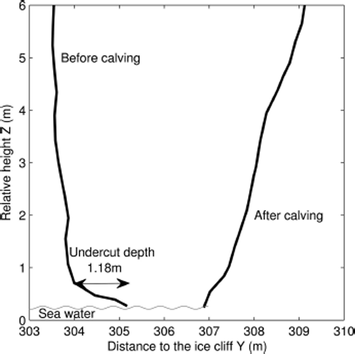
Fig. 11. Cross section of the calving front face on Hansbreen before and after the calving event on 31 July 2012, with measured depth of the undercut at the waterline. The Y-axis is normal to the front surface, increasing inland, and the Z-axis is vertical.
Calving activity and environmental forcing
In summer 2012 the calving activity of Hansbreen front was significantly higher than in 2011 (Fig. 12). In 2011 there were only two days with calving activity >30% of the width of the glacier (Fig. 12). The highest calving activity occurred on 13 August 2011, when changes were registered at 36% of the width of the ice cliff. In 2011 there were nine days with no calving registered. In the summer of 2012 there were 11 days with calving activity >30% of the width of the ice cliff (Fig. 12). The largest changes occurred on 21 August 2012, when the calving activity reached 66% of the glacier width. In contrast to the previous summer, calving events were registered every day of the 2012 summer season.

Fig. 12. Calving activity of Hansbreen and ice velocity in (a) 2011 and (b) 2012, melt rate in (c) 2011 and (d) 2012, and undercut notch melt rate in (e) 2011 and (f) 2012. Note the gap in the calving activity record from 18 June to 25 July 2012, due to the failure of the time-lapse camera. (Date format is dd/mm/yyyy.)
The ice flow velocities of Hansbreen at ablation stake II were relatively stable in summer 2011, ranging from 0.02 to 0.06 m d−1, with maximum values in the second half of June and a minimum at the beginning of August (Fig. 12a). In summer 2012 the ice velocities were similar (0.02–0.08 m d−1), with two peaks in late June and August (Fig. 12b). Unlike the ice velocities, the calving activity was very different for these years, being relatively stable in 2011 and variable and increasing over the course of summer 2012. The correlation coefficient between ice-flow changes and calving activity fluctuations cannot be determined, but it is clear the behaviour in 2011 is different to that in 2012.
The ablation measured at stake II was slightly lower in summer 2011 than in 2012 (Fig. 12c and d). In summer 2011 ablation increased from June to mid-July, following the air temperature rise (Fig. 2). There was then a significant decrease in ablation in the period when the ice pack was present in the fjord, July 2011, that coincided with very low calving activity (Fig. 12c). After that, the ablation and calving activity increased again. In summer 2012 lower ablation coincided generally with lower calving activity, but given the low temporal resolution of the mass-balance measurements no obvious relationship can be observed (Fig. 12d).
The modelled undercut melt rate more closely followed the observed changes in calving activity for both 2011 (Fig. 12e) and 2012 (Fig. 12f). While ice pack was present in the fjord (mid- to late July 2011), when the modelled undercut melt rate was close to zero, calving activity was also very low (Fig. 12e). At the time of strong westerly winds in August 2012 (Fig. 3) both the undercut melt rate and the calving activity were higher than average (Fig. 12f).
The scatter plot of surface ablation and calving activity shows a weak linear relationship between these two variables (Fig. 13a). The points related to both investigated summer seasons are well mixed and do not show significant clustering. The calving activity is not linearly dependent on ice flow velocities (Fig. 13b). There is a very strong linear relationship between the modelled undercut notch melt rate and the calving rates averaged over the same periods of time as the ablation and ice velocity measurements (Fig. 13c), but it is based on only eight points. A linear relationship is also apparent between calving activity and air temperature (Fig. 13d), but not between calving activity and the sum of daily precipitation (Fig. 13e). However, the most pronounced linear dependency for daily values is that between calving activity and the undercut notch melt rate (Fig. 13f). Separate clusters can be seen in data for 2011 and 2012, with the former concentrated at lower and the latter at higher values of both variables.

Fig. 13. Scatter plots of Hansbreen calving activity in summer 2011 and 2012 and (a) ablation, (b) ice velocity, (c) undercut notch melt (averaged over the same periods as ablation and ice velocity), (d) daily mean air temperature, (e) daily sum of precipitation (only days when precipitation occurred) and (f) daily undercut notch melt rate.
The correlation coefficients between calving activity and the rate of thermal erosion in the abrasive notch were much higher than with the other analysed environmental forcings, i.e. air temperature, precipitation, surface ablation and ice flow velocity (Table 2). When considering the daily calving activity and the daily values of environmental forcings (i.e. not the ones averaged over the same periods of time as the ablation and ice velocity measurements), the highest correlation coefficients for the undercut notch melt rate a day before (0.78) can be observed. When the time lag is increased by another day the correlation decreases. It should be noted that the correlation coefficient remains higher than for the other environmental forcings even when the same time averaging is applied, i.e. if means over the same periods of time as the measurements of ice flow velocity and surface ablation are considered. The correlation coefficients with air temperature and ablation are also quite high, reaching values of 0.67 and 0.63, respectively, for the averaged calving activity and dropping to ∼0.4 for daily values.
Table 2. Pearson’s correlation coefficients between the calving activity and modelled undercut notch melt rate, surface ablation, ice velocity of Hansbreen, air temperature and precipitation during the summers of 2011 and 2012. The number of points used for each correlation calculation is given in square brackets

Discussion
The lower calving activity in 2011 may be associated with the persistent presence of an ice pack in Hornsund fjord in July 2011 (Reference KruszewskiKruszewski, 2012). The ice pack reduced the wave height and the sea-water temperature and, thus, the calving intensity. The meteorological conditions and ice flow velocities were similar in 2011 and 2012; the only significant difference in the forcing of calving was the inflow of cold waters and the presence of an ice pack in 2011.
Advections of warm air masses from the west are common phenomena in the Hornsund region (Reference Niedźwiedź, Marsz and StyszyńskaNiedźwiedź, 2013) and they cause a switch of the prevailing wind direction from east to west (Reference Styszyńska, Marsz and StyszyńskaStyszyńska, 2013). Due to the topography, western winds allow oceanic waves and the swell of the Greenland Sea to enter the fjord. This high-energy wave action significantly increases the thermoerosion at the waterline, causing rapid development of the notch during these events. Afterwards, the calving activity increases significantly (Fig. 12). The increase in average wave height stimulated the occurrence of especially large calving events, as a result of enhanced heat exchange between water and ice. Melting of polycrystalline glacier ice is more intense at the crystal or grain boundaries (Reference Shumskiy and KrausShumskiy, 1964). This promotes disintegration of ice, subsequent mechanical removal of loosened crystals by waves and, thus, thermal abrasion of the notch in the ice cliff.
It can be argued that the change in calving activity could be explained by increased water supply to the crevasses and glacier bed caused by rainfall and surface melt (Reference Benn, Warren and MottramBenn and others, 2007a). However, no significant surface melt increase (Fig. 12; Table 2) was observed during these episodes. Moreover, the correlation coefficient between calving activity and the undercut notch melt rate is higher than that between calving activity and measured ablation, ice velocity, air temperature and precipitation. While the correlation with air temperature and ablation is relatively high, compared with the precipitation and ice velocity, this might be partly due to the dependency of the undercut notch melt rate on air temperature.
The presence of large waves shortly after the intensive calving could increase the rate of thermal abrasion; however, the time span when these waves are excited is too short to produce significant erosion of the cliff. Therefore, no positive feedback between calving and enhanced thermal abrasion through an occurrence of a glaciogenic wave was observed.
Our observations imply that calving on Hansbreen is usually triggered by a local imbalance of forces at the front, due to its undercutting at the sea waterline and development of the notch. As the notch gets deeper, the local imbalance of forces above it causes small calving events in the lower part of the cliff face that further decrease its stability (Fig. 14). The vertical fracture at the back of the calving block of the ice usually follows existing crevasses to some depth, but then new fracturing takes place. This suggests that the water-filled crevasse propagation depth proposed in existing state-of-the-art models as the main criterion for triggering calving is not valid in this case. Contrary to previous work, we suggest that the calving rate is controlled by undercut melt at the waterline and calving itself is facilitated by pre-existing fractures developed by longitudinal stretching of the ice in the terminal part of the glacier. This mechanism also explains the lack of calving activity during the winter, and shows why calving activity starts after warming of ice-free surface sea water or an inflow of warm oceanic water into the adjacent bay. The growth of the undercut notch is most rapid in the ice cliff sectors above subglacial channel outflows that cause upwelling and therefore increase the heat flux from warm oceanic water. This leads to an increase in calving rates and a faster retreat rate in the vicinity of subglacial outflows. Unfortunately insufficient data are available to provide a precise estimate of the increase of the melt rate in these areas of Hansbreen, but the presence of the ice gates above the subglacial outflows shows this rate to be significant, although spatially limited to this specific area.

Fig. 14. Hansbreen ice cliff with small overhangs due to calving above the undercut notch (marked with C). Photograph taken using a time-lapse camera on 20 June 2010.
An example of a detailed survey of a calving event on 31 July 2012 shows that the vertical profile of the ice cliff after calving does not follow a strictly vertical shape (Fig. 11). The undercut notch depth before calving is approximately equal to one-third of the depth of the calved ice block measured at the water level. The slope of the ice cliff in the lower part then reverses, from overhanging to sloping towards the sea (Fig. 11). The lower part of the new ice cliff surface shows clean blue ice, with no visible traces of ablation, sediments or old snow trapped within the crevasse during the winter. This contradicts the theory of the mechanism of calving due to longitudinal stretching caused by the acceleration of ice near the front, where the crevasses open gradually during ice flow towards the ice cliff.
The discrepancies between the modelled (Fig. 9d) and measured (Fig. 10b) undercut notch depths are significant. The maximum cumulative measured depth over the period 31 July–19 August 2012 was 22% lower than the cumulative notch melt. The mean cumulative depth in the westernmost sector of the ice cliff was 43% of the modelled value, whereas for the whole surveyed part of the cliff it was only 23% (Figs 9d and 10b). It can be argued that the lower values of the undercut notch depth in the eastern part of the survey were caused by a poorer-quality return signal, i.e. lower intensity of the reflected laser beam due to the greater distance to the ice cliff. These discrepancies can be explained by two factors: underestimation of the measured cumulative undercut notch depth, due to the low sampling rate and overestimation of the modelled melt rate, due to an imprecise parameterization of the model. The model parameters (the empirical constant coefficient of 0.000146 and the roughness length, R) need to be tuned to the local conditions if enough validation data are available. However, given the large variation in the observed rate of notch cutting (Fig. 10), the high quality of the validation of these parameters reported by Reference El-Tahan, Venkatesh and El-TahanEl-Tahan and others (1987) and that they were kept unchanged in the work of Reference Vieli, Jania and KolondraVieli and others (2002), it seemed most appropriate to apply this original set of parameters, to allow direct comparison of the model results with former studies. Obviously, this may be an important source of the observed discrepancy between the modelled and measured melt rates; however, given the simple form of the model (Eqn (1)) and a relatively small amount of gathered observational data that could be used to calibrate it, the parameters have not been changed. Nevertheless, as the relationships of the model are linear or almost linear, this discrepancy should not change the interpretation of the obtained results.
The sensitivity analysis of the undercut notch melt model shows that the melt was more sensitive to water temperature changes in 2011 and to wave height changes in 2012 (Fig. 9). In summer 2011 the sea-surface temperature was relatively low and the waves were higher than in summer 2012 (Fig. 7). Therefore ΔT was low, as T a was close to T fp. Given the linear relationship between the undercut melt rate, V m, and ΔT (Eqn (1)), a relatively large change in ΔT, in this case ±1°C, resulted in a substantial change in the modelled melt rate. The same pattern was predicted for the model sensitivity to the wave height in 2012. This result suggests that calving rates are highly sensitive to sea-water temperature changes when close to the freezing point.
The undercut melt rates calculated in this study are lower than the 1 m d−1 value proposed by Reference Vieli, Jania and KolondraVieli and others (2002). The main reason is that here field measured values of the water temperature, wave height and period were used, while Vieli and others only roughly estimated these variables. Another issue is that in the study of Reference Vieli, Jania and KolondraVieli and others (2002) the undercut melt rate was equal to the calving rate caused by the imbalance of forces, due to the undercutting at water level, i.e. this type of calving was associated only with the break-off of ice slabs directly above the notch. Here we show that it can also trigger calving events at greater depth, even up to twice the undercut notch depth. It could therefore be speculated that the calving rates might be equal to at least twice the melt rate of the undercut, which stays in accordance with the modelling studies (Reference O’Leary and ChristoffersenO’Leary and Christoffersen, 2013).
The size and dynamics of Hansbreen are typical of a Svalbard grounded tidewater glacier; however, it should be noted that the processes observed there may not be significant for larger glaciers. This may be the case for floating or semi-floating glaciers, where submarine melt at the grounding line can trigger large calving events, which do not occur on smaller glaciers such as Hansbreen. Nevertheless, undercutting at the waterline may be of great importance for calving of grounded tidewater glaciers of comparable size to Hansbreen.
Conclusions
The main conclusion of this study is that calving on Hansbreen grounded tidewater glacier is mainly triggered by the local imbalance of forces at the front, due to undercutting at the sea waterline and development of a thermo-erosional notch. There is a strong correlation between the observed calving activity and the modelled ice melt at the waterline. This correlation is particularly strong for a one-day lag between calving activity and the melt rate, indicating the importance of the mechanical destabilization of the ice front by the undercut. A large part of the fracturing associated with calving takes place just next to the calving front, which contradicts the theoretical mechanism of gradual stretching of crevasses due to acceleration of ice flow in the frontal part, and their deepening by the presence of water. In summer 2011 the presence of dense drifting sea-ice floes in Hornsund fjord drastically decreased the calving intensity of Hansbreen, by cooling surface water and suppressing wave action. Hansbreen and tidewater glaciers of the western coast of Svalbard are sensitive to atmospheric advection from the west, due to the associated influx of warmer sea water and increased wave activity, causing more rapid development of the thermo-erosional notch at sea level and, hence, calving. It can be expected that calving rates of the tidewater glaciers of Svalbard will rise with increased advection of warmer Atlantic waters to the Arctic.
Author Contribution Statement
M.P. performed all calculations, collected TLS, ice velocity and mass-balance data and wrote most of the paper; M.C. investigated calving activity and surface sea-water properties; J.A.J. designed the study of the undercut notch; A.P. provided CTD data and C.K. helped in writing this paper.
Acknowledgments
We thank the crew of Polish Polar Station Hornsund for their support with fieldwork. We also thank J. Abermann for valuable comments that helped to improve the manuscript. The studies were partly funded by the statutory activity of the Institute of Geophysics, Polish Academy of Sciences, Polish National Science Center grant DEC-2013/11/N/ST10/00823, Polish–Norwegian Fund projects AWAKE (PNRF-22-AI-1/07) and AWAKE2 (Pol-Nor/198675/17/2013). The publication has been partially financed by the Centre for Polar Studies from the funds of the Leading National Research Centre (KNOW) in Earth Sciences (2014–18).


 Open access