


1. INTRODUCTION
Glaciers in the Karakoram mountain range are an important source of freshwater for one of the most densely populated river basins (Indus Basin) in the world (Immerzeel and others, Reference Immerzeel, Pellicciotti and Bierkens2013). The volume of discharge generated by snow and glacial melt far exceeds the volume of the discharge generated in the downstream areas of the basin (Immerzeel and others, Reference Immerzeel, van Beek and Bierkens2010). The status of glaciers in the Karakoram has a direct impact on some of the key components of the global water cycle, global mean sea-level rise (Gardelle and others, Reference Gardelle, Berthier and Arnaud2012), freshwater availability and the risk of Glacial Lake Outburst Floods and droughts. Besides, continuous monitoring of glaciers is crucial for identifying the regional impacts of changing climate (Bolch and others, Reference Bolch2012), particularly where long-term climatic measurements are rare.
Components of glacier mass budget have been monitored throughout the world for more than six decades (WGMS, Reference Zemp2008; Zemp and others, Reference Zemp, Hoelzle and Haeberli2009). As a result, various measurement methods have evolved with their own sets of merits and demerits (Hoinkes, Reference Hoinkes1970). For example, field-based glaciological methods (Mayo and others, Reference Mayo, Meier and Tangborn1962; Kaser and others, Reference Kaser, Fountain and Jansson2002) are widely used but are extremely manpower intensive. Inevitably, field-based methods in the Himalaya are biased towards short-term assessment of certain glaciers, such as Chhota Shigri (Wagnon and others, Reference Wagnon2007; Azam and others, Reference Azam2014), which are easy to access and smaller in size. Similarly, the accumulation area method suggested by Kulkarni and others (Reference Kulkarni, Rathore, Singh and Bahuguna2011) uses empirical, field-based relationships and can only be extrapolated to glaciers that lie within a certain climatic region (Kulkarni and others, Reference Kulkarni, Rathore and Alex2004). Geodetic methods, comparing DEMs from at least two different times, have been extensively implemented for various regions around the globe, including Karakoram glaciers (Gardelle and others, Reference Gardelle, Berthier and Arnaud2012), Lahaul Spiti glaciers (Berthier and others, Reference Berthier2007), glaciers in Khumbu Himalaya (Bolch and others, Reference Bolch, Pieczonka and Benn2011; Nuimura and others, Reference Nuimura, Fujita, Yamaguch and Sharma2012), the Tien Shan (Bolch, Reference Bolch2015; Pieczonka and Bolch, Reference Pieczonka and Bolch2015) and in general for Pamir-Karakoram-Himalayan glaciers (Gardelle and others, Reference Gardelle, Berthier, Arnaud and Kääb2013). In contrast, the hydrological mass budget method involves subtracting hydrological outputs (i.e. evaporation and runoff) from hydrological inputs (i.e. mass gain from snowfall) for a glacier in order to determine its mass budget. This method has been rarely used in the Himalaya since Bhutiyani (Reference Bhutiyani1999).
The Karakoram Range, comprising ~18 800 km2 of glacier area (Bolch and others, Reference Bolch2012), accounts for nearly 3% of the total area of ice outside the ice sheets in Greenland and Antarctica (Cogley, Reference Cogley2012). Even though Karakoram glaciers have shown irregular behavior over longer time periods, they have retreated on average over most of the 20th century (from 1920 to 1990) (Hewitt, Reference Hewitt2005). Further, earlier reported expansion of high-relief glaciers in the Karakoram (Hewitt, Reference Hewitt2005) was later negated by Bhambri and others (Reference Bhambri2013) and Minora and others (Reference Minora2016), who reported heterogeneous glacier behavior but on average no significant change in the Upper Shyok Valley, NE Karakoram since 1970 and in Central Karakoram since 2000. Owing to the political sensitivity and logistic difficulties of the Karakoram region, studies of glacier dynamics (Copland and others, Reference Copland2009; Scherler and others, Reference Scherler, Bookhagen and Strecker2011) and mass budget (Gardelle and others, Reference Gardelle, Berthier and Arnaud2012; Kääb and others, Reference Kääb, Berthier, Nuth, Gardelle and Arnaud2012) have been primarily based on satellite observations. Earlier studies of glacier dynamics in the Eastern Karakoram ranges have reported increases in surface velocity (Heid and Kääb, Reference Heid and Kääb2012) with average stable termini (Scherler and others, Reference Scherler, Bookhagen and Strecker2011; Bhambri and others, Reference Bhambri2013). Also, a large number of surge-type glaciers have been reported in the Karakoram since the 1860s (Barrand and Murray, Reference Barrand and Murray2006; Copland and others, Reference Copland2011). And perhaps most interestingly, surge activity has increased in recent years (e.g. Copland and others, Reference Copland2011; Quincey and others, Reference Quincey2011; Rankl and others, Reference Rankl, Kienholz and Braun2014). Gardelle and others (Reference Gardelle, Berthier and Arnaud2012), based on remotely sensed geodetic measurements over 5615 km2 of glacierized area in the central Karakoram, computed a region-wide mass budget of 0.11 ± 0.22 m w.e. a−1 for the period of 1999–2010. More specifically, the mass budget of surging and non-surging glaciers was reported to be 0.11 ± 0.31 m w.e. a−1 and 0.10 ± 0.19 m w.e. a−1, respectively. Thus, the Karakoram glaciers were either in equilibrium or gaining mass between 1999 and 2010 (Gardelle and others, Reference Gardelle, Berthier and Arnaud2012, Reference Gardelle, Berthier, Arnaud and Kääb2013). Like many other Himalayan and Karakoram glaciers, Siachen Glacier has not been monitored adequately owing to remoteness and years of military conflict in the area. Bhutiyani (Reference Bhutiyani1999) made an independent study of hydrologic mass budget for Siachen Glacier during 1986–1991 and obtained a large negative mass budget of −0.51 m w.e. a−1. However, Zaman and Liu (Reference Zaman and Liu2015) made corrections to the catchment area of Siachen Glacier and found mass budget values with upper and lower bounds of +0.22 m w.e. a−1 and −0.23 m w.e. a−1, respectively. However, since the hydrological method involves differencing of hydrologic variables with large magnitudes such as runoff, evapotranspiration and precipitation over the entire catchment, it is prone to large relative errors making the method less reliable (Zaman and Liu, Reference Zaman and Liu2015). The study by Gardelle and others (Reference Gardelle, Berthier, Arnaud and Kääb2013) also covered Siachen Glacier. The authors reported a slightly positive mass budget of +0.14 ± 0.14 m w.e. a−1 during the period 2000–10. This estimate is however uncertain because of incomplete coverage of the glacier.
To our knowledge, the present study presents the most comprehensive assessment of Siachen Glacier in terms of its mass budget, velocity and area. The specific aims of this study include: (1) analysis of changes in the area of Siachen Glacier (2) improving understanding of how surface mass budget affects the surface velocity pattern and thickness variations of the glacier; of particular interest, in this regard, are differences between the elevation changes of exposed and debris-covered ice (3) quantitative characterization of mass budget for Siachen Glacier utilizing high-precision, remote sensing-based geodetic techniques.
2. STUDY AREA
Siachen Glacier is the largest glacier in the entire Karakoram Range and extends between the latitudes of 35°10′N-35°42′N and longitudes 76°46′E-77°25′E (Fig. 1). It spans a length of ~74 km and its width varies between 1 and 8 km, covering an area of ~936 km2 with an estimated mean thickness of ~300 m (Frey and others, Reference Frey2014). This makes Siachen the largest glacier not only of the Karakoram but also of all of High Mountain Asia. This glacier is located near the political boundary between India and Pakistan, in the eastern part of the Karakoram Range.
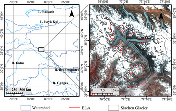
Fig. 1. Location of Siachen Glacier. Inset shows complete area of Siachen Glacier. The red line shows the ELA of 5250 m.
Siachen Glacier lies within the altitude range of 3400–7300 m a.s.l. with an average elevation of 5500 m a.s.l. Westerlies are an important source of precipitation for the Karakoram including Siachen Glacier. Nearly two-thirds of the annual snowfall in these areas occurs under the influence of extra tropical cyclones known as western disturbances, primarily during the winter season (Bhutiyani, Reference Bhutiyani1999).
3. DATA
3.1. Cartosat-I
The Cartosat-I (IRS-P5) sensor is ideally suited for DEM generation in glaciological terrains, offering a base to height ratio of 0.62, a radiometric resolution of 10 bits and a spatial resolution of 2.5 m (Tiwari and others, Reference Tiwari, Pande, Punia and Dadhwal2007; Bolch and others, Reference Bolch, Pieczonka and Benn2011; Pieczonka and others, Reference Pieczonka, Bolch and Buchroithner2011). The time difference between acquisitions of the members of stereo image pairs is 52 s, ensuring minimal temporal aliasing, which is particularly important for glaciological applications. In this study, three Cartosat-I images (Table 1) with an overlapping area of 98 km2 were used to get an almost complete coverage of Siachen Glacier. The Cartosat-I ortho-pair was radiometrically corrected and coarsely geolocated using the path–row referencing system, which gives a horizontal accuracy of 170–300 m (Gianinetto and Fassi, Reference Gianinetto and Fassi2008; Pieczonka and others, Reference Pieczonka, Bolch and Buchroithner2011). Rational polynomial coefficients (RPCs), also provided for each image of the stereo pair, were used to define the mathematical relationship between pixel and ground coordinates more accurately (Titarov, Reference Titarov2008). Since no field study could be conducted and no topographical maps are available, we have processed the Cartosat- I DEM without ground control points (GCPs).
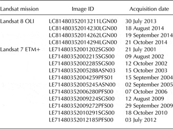
Table 1. Details of the optical image datasets used
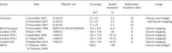
Also included is the SRTM.
* Used for glacier mapping in places of non-coverage of Cartosat-I scenes.
3.2. Landsat
In this study we utilized Landsat L1T products, which provide improved radiometric, geometric (by incorporating GCPs) and topographic accuracy (by employing DEMs) and a gap-filled Landsat scene obtained on 12 August 2009 from www.landsat.org. For glacier mapping, nearly cloud free scenes (cloud cover <30%) acquired at the end of the ablation period (starting from July to August) with minimal seasonal snow were used (Table 1).
3.3. KH-9 hexagon mapping camera (MC)
The KH-9 program (code-named Hexagon) of the US military, operational from 1973 to 1980, was aimed at reconnaissance and map making. In 2011, KH-9 images of the frame-MC with a resolution of 20–30 ft (~6–9 m), a frame of 23 × 46 cm2 and a focal length of 30.5 cm (Surazakov and Aizen, Reference Surazakov and Aizen2010; Padmanabha and others, Reference Padmanabha, Shashivardhan Reddy, Narender, Muralikrishnan and Dadhwal2014) were declassified. The KH-9 scene used in this study (Table 1) covers an area of ~161 × 241 km2, is mostly cloud free and has good image contrast for glacier mapping.
3.4. Envisat Advanced Synthetic Aperture Radar (ASAR), Japanese Advanced Land Observing Satellite Phased Array-type L-band (ALOS PALSAR) and Shuttle Radar Topography Mission (SRTM)-DEM
The ASAR is onboard the ENVISAT satellite launched in 2003. The ASAR operates in the C-band frequency range with a wavelength of 5.66 cm. At this wavelength, cloud cover has no impact on the reflected radar signals (See Table 2 for ENVISAT ASAR scenes used). We have used Envisat ASAR images to delineate debris-covered tongue using coherence mapping.
Table 2. Details of Envisat ASAR images used as pairs for the computation of coherence images
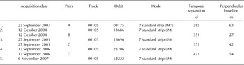
* IM refers to Image Mode.
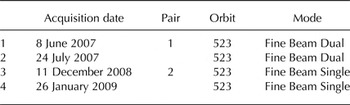
For generating velocity maps, we utilized wintertime ALOS PALSAR data, acquired on 11 December 2008 and 26 January 2009 in fine beam single (FBS) mode and summertime data acquired on 8 June 2007 and 24 July 2007 in fine beam dual (FBD) mode. All acquisitions were along orbit 523 (Table 3).
Table 3. List of ALOS PALSAR datasets used for generating velocity maps
SRTM data have been used as a reference DEM in a number of glaciological studies to generate elevation difference maps by comparing them with recent (Berthier and others, Reference Berthier2007; Paul and Haeberli, Reference Paul and Haeberli2008) and historical DEMs (Surazakov and Aizen, Reference Surazakov and Aizen2006; Schiefer and others, Reference Schiefer, Menounos and Wheate2007; Pieczonka and others, Reference Pieczonka, Bolch, Wie and Liu2013) and with repeat-track ICESAT data (Kääb and others, Reference Kääb, Berthier, Nuth, Gardelle and Arnaud2012; Neckel and others, Reference Neckel, Kropacek, Bolch and Hochschild2014). Here we used the SRTM3 V2 without void filling, which was provided by NASA in 2002 (http://dds.cr.usgs.gov/-srtm/version2_1/SRTM3/) (Table 1).
4. METHODOLOGY
4.1. Estimating the equilibrium-line altitude (ELA)
For estimating the ELA of Siachen Glacier we have assumed that the late-summer snow line altitude (SLA), i.e. the elevation of the snowline at the end of the hydrological year, can be considered as representative of the ELA (Rabatel and others, Reference Rabatel2012). Thereafter, we identified the SLA visually on a number of Landsat images near the end of the ablation period between the years 2000 and 2014 (Table 4). To facilitate the identification of the SLA, we created false-color composites from the short wave infrared (SWIR), near infra-red (NIR) and one visible band (GREEN) and mapped the boundary between bright snow and darker ice (Rabatel and others, Reference Rabatel2012). Since Siachen Glacier has a number of tributary glaciers with different SLAs, we computed the mean SLA from different tributaries. Finally, we averaged the SLAs from the different images to obtain the best estimate of the ELA of 5250 m a.s.l. The accumulation-area ratio was 0.60, which is similar to the value 0.58 mentioned by Hewitt (Reference Hewitt2011).
Table 4. List of Landsat Images used for ELA determination
4.2. Glacier mapping
For creating exposed-ice boundaries using Landsat data products available for 1990, 2000 and 2014, the ratio of RED to SWIR digital numbers is computed, followed by a selection of an appropriate threshold value of 2.1 (Paul and Kääb, Reference Paul and Kääb2005; Bolch and others, Reference Bolch, Menounos and Wheate2010). To overcome noise and isolated pixels in an automated manner, a 3 × 3 median filter was applied. In addition, a few misclassified pixels were edited and deleted manually in order to refine the boundary. The final binary image was converted to a vector shapefile. Cartosat-I stereo scenes with a spatial resolution of 2.5 m, orthorectified on the basis of the Cartosat-I DEM generated in this study, were used to delineate the exposed-ice boundary manually for the year 2007. As the glacier was not entirely covered by the Cartosat-I scenes, we used the gap-filled Landsat ETM+ scene of the year 2009 for delineating the remaining parts.
For mapping Siachen Glacier using Hexagon KH-9 imagery, ~100 tie points (TP) were collected to co-register the image to the Cartosat-I/Landsat ETM+ scene. TPs were obtained both automatically, from the orthorectified Landsat ETM+ metadata file, and manually, from an orthorectified and pansharpened SWIR-NIR-RED (6-4-3) false-color composite from the OLI scene of 2014. A spline transformation, which optimizes for local accuracy, was used to reference the images based on the TPs. Utilization of this technique with a large number of well-distributed TPs yielded a good accuracy (in the order of 3–4 m) for the entire study area. Thereafter, this georeferenced Hexagon image was orthorectified using the SRTM DEM of 30 m resolution with the Create Ortho-Corrected Dataset module in ArcGIS in order to correct for geometric distortions.
Debris-covered ice was mapped manually using Landsat color composites (SWIR, NIR, RED) for the years 1990, 2000 and 2014. High-resolution orthorectified Cartosat-I (along with the gap-filled Landsat image) and Hexagon imagery was used to manually delineate debris-covered ice boundaries for the years 2007 and 1980, respectively.
In order to support the identification of the debris-covered tongue and to study changes in snout position, we have used coherence mapping, which relies on high-precision interferometric techniques utilizing SAR data. This method has been effectively used to delineate glaciers automatically (Atwood and others, Reference Atwood, Meyer and Arendt2010), study changes in snout position (Saraswat and others, Reference Saraswat2013) and identify debris-covered portions of glaciers (Frey and others, Reference Frey, Paul and Strozzi2012).
Coherence (γ) is a measure of spatial correlation between two SAR acquisitions. Better coherence results in the generation of high quality interferograms, while loss of coherence results in decorrelation. Changes in vegetation growth, permafrost freezing and thawing, soil moisture content and glacier motion between two SAR acquisitions are some of the pertinent causes of decorrelation.
To assess the changes in the position of the debris-covered snout, coherence maps were generated for the period 2004–08 by processing Envisat ASAR images with JPL/Caltech ROI_pac software using the methodology detailed in Simons and Rosen (Reference Simons and Rosen2007). Saraswat and others (Reference Saraswat2013) estimated that there is a bias of ~20% in the coherence estimates especially in glacierized regions, which have low coherence values. Since the members of the interferometric pairs used in this study were acquired one year apart (Table 2), the glacierized region is affected by motion-related decorrelation whereas the ice-free area is free from this effect. Thus the area near the glacier snout, where the ground is exposed, shows better coherence in contrast to the pixels of the surrounding glacier (Atwood and others, Reference Atwood, Meyer and Arendt2010; Frey and others, Reference Frey, Paul and Strozzi2012). The stable areas ahead of the debris-covered snout have coherences in the range 0.5–0.9 while the glacierized areas have coherence in the range 0.0–0.5. We used a coherence between 0.50 and 0.55 (depending on the scene) to delineate the debris-covered tongue. Comparison of the boundary generated using coherence mapping with that created manually reveals good fit between the two (Figs 2a–d). Hence, this method can be particularly important to quantify changes in terminus position for heavily debris-covered glaciers in a semi-automated manner, since manual mapping of debris-covered glacier tongues requires high-resolution datasets, which can be difficult to obtain.
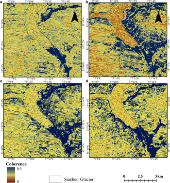
Fig. 2. Coherence images from Envisat ASAR data used to validate the manual mapping and to delineate debris-covered tongue for different years. Shown by the black line is the debris-covered tongue as delineated manually. (a–d) Represent the interferometric pairs (Table 2).
4.3. Mapping uncertainty
The precision of automatic delineation of exposed ice is usually within half a pixel (Bolch and others, Reference Bolch, Menounos and Wheate2010; Paul and others, Reference Paul2013). Since no higher resolution datasets are available to manually correct the automatically derived boundaries, mapping uncertainty for the Landsat scenes of 1990, 2000 and 2014 was calculated by using a buffer distance of 15 m around the automatically derived boundaries. For manually delineated boundaries using the Hexagon scene of 1980, we assumed a mapping uncertainty of ~8 m (i.e. 1 pixel) (Pieczonka and others, Reference Pieczonka, Bolch, Wie and Liu2013). In the case of 2007 glacier boundaries, delineated using Cartosat-I images, a mapping uncertainty of 2.5 m (1 pixel) is assumed. For the area not covered by the Cartosat-I image, an error estimate of 15 m was used, similar to that of Landsat images. Overall, this resulted in an uncertainty of 1.82% of the total exposed-ice area of Siachen Glacier mapped for the year 2007 (Table 5).
Table 5. Changes in area and length of Siachen Glacier, 1980–2014
4.4. Generation of velocity map
The offset field between pairs of ALOS PALSAR satellite data acquired with a 46-day interval was used for the estimation of glacier velocities. Offset tracking of L-band SAR images is a robust and direct technique for estimating glacier motion (Rignot, Reference Rignot2008; Strozzi and others, Reference Strozzi, Koureav, Wegmülle, Sharoy and Werner2008; Pohjola and others, Reference Pohjola2011). This is particularly useful when Differential Interferometric Synthetic Aperture Radar (DInSAR) is limited by the loss of coherence due to long time intervals.
Offset tracking measurements made along the slant-range (incidence angle is ~35° for ALOS PALSAR observations) and azimuth directions are combined to retrieve horizontal displacements on the ground. Slant-range and azimuth offset estimation errors of ALOS PALSAR data are in the order of one tenth of a pixel. For a FBS with ground-range pixel spacing of 7.5 m and an azimuthal pixel spacing of ~3 m, two-dimensional (2-D) ice velocities can be computed with an expected error of 0.8 m in 46 days or ~10 m a−1. For a FBD with ground-range pixel spacing of ~15 m, 2-D ice velocities can be computed with an expected error of 20 m a−1. The displacement maps were geocoded to geographical coordinates with the WGS84 horizontal datum and the EGM96 vertical datum at 90 m resolution, using the SRTM Digital Elevation Database v4.1 (Jarvis and others, Reference Jarvis, Reuter, Nelson and Guevara2008).
4.5. DEM generation and co-registration
All Cartosat-I scenes of the year 2007 were pre-processed using PCI Geomatica OrthoEngine 10.2. Data pre-processing involved radiometric enhancements using a locally-adaptive Wallis filter, which adjusts the brightness of greyscale images in local areas as opposed to other global filters (Pieczonka and others, Reference Pieczonka, Bolch, Wie and Liu2013). This adjustment was very critical for shadow regions and accumulation areas of glaciers since they lack sufficient contrast, causing errors in parallax determination.
The next step in DEM generation was to compute the satellite stereo model, in order to determine the ground position of each point in the stereo scene. Cartosat-I scenes are provided with RPCs (Titarov, Reference Titarov2008). Even though these RPCs can be improved further using GCPs, sub-pixel horizontal accuracy can only be achieved when the GCPs are at least two or three times more accurate than the spatial resolution of the satellite image (Höhle and Höhle, Reference Höhle and Höhle2009). For Cartosat-I data with 2.5 m resolution, the required horizontal accuracy of GCPs should be in the range 1–1.5 m, which for all practical purposes can only be achieved with in-situ measurements. Therefore we have not used any GCP during the preparation of the Cartosat-I DEM.
The Cartosat-I DEM was geocoded in the Universal Transverse Mercator (UTM) system; zone 43 N, with a grid size of 30 m. The SRTM DEM was projected into the UTM coordinate system and then resampled bilinearly from 90 m to 30 m resolution in order to make it conformable with the Cartosat-I DEM. About 7.5% of the glacier area in the accumulation zone is not covered by the Cartosat-I DEM (Fig. S1). To identify the outliers caused due to Cartosat-I DEM failure, hillshaded images of the Cartosat- I DEM and SRTM DEM were compared. The outliers on the glacier surface seen as black patches in the uppermost accumulation area in Figure S1 were removed before further processing.
4.6. Co-registration of DEMs
DEM differencing necessitates co-registration to ensure that corresponding pixels in the two DEMs represent the same ground location.
According to Nuth and Kääb (Reference Nuth and Kääb2011), elevation difference, slope and aspect of non-glacierized pixels are related by the following equations:
 $${\rm dh} = a \cdot \tan \alpha \cdot \cos \;(b - \psi ) + \; {\rm dh}{\rm ^{\prime}}$$
and dh, α and ψ represent elevation differences at individual pixels, terrain slope and aspect, respectively. The terms a, b, dh′ denote the magnitude of the horizontal shift, the direction of the shift vector and the overall elevation bias between the two DEMs.
The parameters a, b and dh′ are computed by least-squares optimization. These values were used to adjust the Cartosat-I DEM iteratively until a maximum of 10 iterations was reached or until the horizontal offset a was <1 m. Residual elevation differences over stable non-glacierized areas due to rotation and scale distortions were minimized by second-order spatial trend corrections (applied to the Cartosat-I DEM). In this process a second-order trend surface was calculated for all ice-free areas and added to the DEM (Pieczonka and others, Reference Pieczonka, Bolch and Buchroithner2011).
4.7. Accuracy assessments
4.7.1. Uncertainty of the mosaicked Cartosat –I DEM
We used the overlapping area (~98 km2) of the three Cartosat-I scenes to quantify the uncertainty in the final mosaicked DEM. Considering the differences between each individual scene to be independent and using the principle of error propagation, we computed a RMSE of ±1.2 m in the final mosaicked Cartosat-I DEM and this was considered as the uncertainty of the mosaicked DEM.
4.7.2. Relative vertical accuracy
In order to quantify the accuracy of the relative fit between the reference DEM (SRTM) and Cartosat-I DEM we computed the mean and standard deviation for ice-free stable areas (Table 6). The mean was taken as a quantitative estimate of the bias due to inaccuracies in the coregistration of the DEMs. Since DEM errors increase with increasing slope (Jacobsen, Reference Jacobsen2005) we restricted the accuracy assessment to regions with slopes <30° (Pieczonka and others, Reference Pieczonka, Bolch and Buchroithner2011). Elevation differences outside the range of mean ±3σ were considered as outliers (Gardelle and others, Reference Gardelle, Berthier, Arnaud and Kääb2013). The statistics for the unadjusted DEM (Table 6) reveal that the removal of outliers significantly reduced both the bias and the standard deviation. The adjusted DEM shows significant improvement in the standard deviation (with and without outlier removal), which reflects a good fit of the two DEMs after co-registration. The bias after removal of outliers was subtracted from the elevation differences over glacierized terrain.
Table 6. DEM difference error statistics before and after co-registration
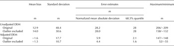
For the quantification of uncertainty we computed the normalized median absolute deviation and the 68.3% quantile for elevation differences over stable ice-free areas. Because of large differences in these two error estimates and the non-normal distribution of the elevation differences over stable areas we chose the 68.3% quantile as a conservative estimator for elevation difference errors (Höhle and Höhle, Reference Höhle and Höhle2009). The 68.3% quantile was added to the error of the mosaicked Cartosat-I DEM to yield a final error estimate of ±2 m for the entire study area (Table 7).
Table 7. Estimates of elevation change and mass budget for Siachen Glacier for 1999–2007
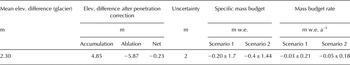
In Scenario 1, a constant density of 850 ± 60 kg m−3 was considered while in scenario 2 densities for accumulation and ablation areas were 600 and 900 kg m−3, respectively.
4.7.3. Correction for C-band penetration and curvature correction
It is crucial to make adequate corrections for the penetration depth of the SRTM's C-band radar beams into snow and ice (Gardelle and others, Reference Gardelle, Berthier and Arnaud2012; Kääb and others, Reference Kääb, Berthier, Nuth, Gardelle and Arnaud2012). The penetration depth, however, depends mostly on the properties of the snow and ice. In the accumulation zone, C-band radar can easily penetrate through the snow, which accumulated on the surface of the previous ablation period and even into the different firn layers of the previous years, which can easily have a thickness of several tens of meters (Huss, Reference Huss2013). On the contrary, C-band radar penetrates much less into the ice of the ablation region. Therefore it is necessary to make elevation-dependent corrections to the SRTM DEM in order to obtain the most precise estimates of glacier surface elevation. Moreover, since C-band radar penetrates well through snow, we have considered the SRTM DEM to be representative of the ablation surface at the end of the previous melt season (i.e., October 1999, Berthier and others, Reference Berthier, Arnaud, Vincent and Rémy2006; Paul and Haeberli, Reference Paul and Haeberli2008). Even though the penetration of X-band radar (with a wavelength of 3.1 cm) into snow may not be negligible (Seehaus and others, Reference Seehaus, Marinsek, Helm, Skvarca and Braun2015), it is significantly less in comparison to C-band radar (with a wavelength of 5.6 cm).
Thus, a comparison between SRTM-X and SRTM-C permits an estimate of the elevation dependency of the C-band penetration (Gardelle and others, Reference Gardelle, Berthier and Arnaud2012). Since SRTM-X did not cover Siachen Glacier, we computed elevation differences between SRTM-X and SRTM-C over nearby glaciers of the Eastern and Western Karakoram Range. A relationship between penetration correction and altitude was thus formulated (Fig. 3). The resulting C-band penetration depths, which increase from ~0.5 m to at least 6.5 m over the elevation range of the glacier, were subtracted on a pixel-by-pixel basis from the elevation differences (Cartosat-I DEM minus SRTM DEM) in order to get the “true” elevation differences. This approach is different from that of Kääb and others (Reference Kääb, Berthier, Nuth, Gardelle and Arnaud2012), who used an average penetration correction of 2.4 ± 0.3 m for the Karakoram glaciers. Our average penetration correction of 3.2 m for Eastern and Western Karakoram glaciers is similar to the average penetration of 3.4 m computed over Karakoram glaciers by Gardelle and others (Reference Gardelle, Berthier, Arnaud and Kääb2013). We could not perform any curvature correction since Siachen Glacier is a gently sloping glacier (average slope of 13°) with most of the area having maximum curvature values between −1 and 0 (Gardelle and others, Reference Gardelle, Berthier and Arnaud2012).
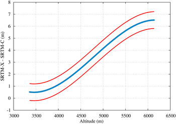
Fig. 3. Smoothed difference between SRTM-X and SRTM-C (blue line), which was applied to correct the penetration of the C-band radar beam. Also shown is the ±1 standard deviation confidence region (red lines).
4.8. Calculation of elevation and mass changes
The elevation differences obtained after DEM and penetration correction were averaged within 100 m altitude intervals (from 3400 to 7300 m), and the average elevation change for the entire Siachen Glacier was computed as an area-weighted average of elevation change in each altitude range. The same procedure was followed to calculate the average elevation changes for the ablation and accumulation regions.
The average elevation change obtained can then be multiplied by suitable densities to obtain mass change estimates. In this study, we have used two density scenarios: (i) density of 850 ± 60 kg m−3 (Huss, Reference Huss2013) for the entire glacier; (ii) densities of 600 and 900 kg m−3 (Hagg and others, Reference Hagg, Braun, Uvarov and Makarevicha2004; Schiefer and others, Reference Schiefer, Menounos and Wheate2007; Kääb and others, Reference Kääb, Berthier, Nuth, Gardelle and Arnaud2012) for the accumulation and ablation areas, respectively.
5. RESULTS
5.1. Glacier area changes
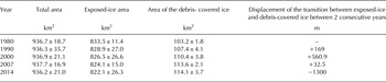
The total area of the Siachen Glacier system was 936.9 ± 21.1 km2 in the year 2000. The area experiences only insignificant variations throughout the study period (Table 5). The exposed-ice area has decreased by 1.3% from 1980 to 2014 while the debris-covered area has increased by 10.5% during the same period (Table 5). Although it is evident that the debris-covered tongue has remained stable over the study period, fluctuations of the boundary between exposed and debris-covered ice are much more prominent. The distal part of this boundary retreated by nearly 1.3 km during the short-time span of 2007 to 2014, even though it remained practically unchanged prior to that (Fig. 4).
5.2. Velocity patterns
Velocity information for almost the entire glacier area could only be obtained for the 11 December 2008–26 January 2009 period, since large parts of the accumulation area suffer from decorrelation during the summer period (8 June 2007–24 July 2007). This temporal decorrelation is most likely due to snowfall between June and July 2007. In general, glacier velocity during the summer acquisition (8 June 2007–24 July 2007) period is greater than the velocity during the winter acquisition (11 December 2008–26 January 2009) period (Fig. 5). However, the general pattern reveals decreasing velocities towards the tongue and very low velocities on the frontal part of the tongue. The greater velocity of Siachen Glacier during summer can be attributed to basal lubrication caused by sub-glacial water flow during the ablation period (Copland and others, Reference Copland2009). The average velocity for the entire glacier during 11 December 2008–26 January 2009 is 12.3 ± 0.4 cm d−1. The average velocities for the accumulation and ablation regions are 9.7 ± 0.4 cm d−1 and 20.4 ± 0.4 cm d−1, respectively. We studied the profiles of glacier velocity for the winter season (11 December 2008–26 January 2009) over the main trunk glacier and the western tributary glaciers, which have shown anomalous behavior (see Table 8). On the main trunk profile AA′ (Fig. 6), velocity in the accumulation region and upper parts of the ablation area (section A) exceeds 40 cm d−1 (Profile AA′, Fig. 7a) and drops steadily in the ablation area (section B) from a maximum at the end of Section A. However, the lower ablation area and areas near the snout (section C) are characterized by a drastic decrease in velocity. All the western tributary glaciers (except the one with profile FF′) have velocities lower than average. The tributary with profile BB′ shows near-zero velocity in most of the accumulation area and lower portions of the ablation area but higher velocity in the middle. While the tributary with profile DD′ shows decreasing velocities throughout its length, those with GG′ and EE′ show relatively low velocities persistent through the entire length of the accumulation and ablation areas.
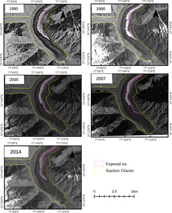
Fig. 4. Extent of exposed-ice on the lower tongue for 1980–2014.
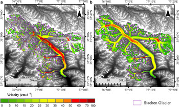
Fig. 5. Velocity pattern over Siachen Glacier for two different seasons: (a) 8 Jun 2007–24 Jul 2007 (b) 11 Dec 2008–26 Jan 2009.
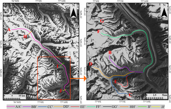
Fig. 6. Map displaying the traces of profile lines used to construct elevation change and velocity patterns for different glaciers. The letters (A–H) in the figure refer to the trace of the particular profile line; for example, letter A refers to the trace of the profile line AA′. Profile lines AA′ to GG′ run from accumulation to ablation area while profile lines HH′ to JJ′ are cross-profiles running from left to right (looking down-glacier).
Table 8. Velocity and elevation change for profiles along the main trunk of Siachen Glacier and selected tributary glaciers
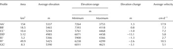
The velocity estimates are for the period 26 January 2009–11 December 2008. Elevation changes, averaged along each profile after correction for C-band penetration are for the period 25 November 2007–11 to 20 October 1999. Uncertainties are ±2.0 m for elevation changes and 0.004 m d–1 for velocities.
5.3. Elevation and mass changes
Elevation changes observed here are spatially heterogeneous with accumulation regions at higher altitudes showing thickening, while ablation zones at lower altitudes show characteristic thinning (Fig. 8). The three tributary glaciers with an area >100 km2 show on average thickening because their accumulation areas are large in proportion to their ablation areas. Over smaller tributaries with an area >50 km2 the average elevation change varies in dependence upon their range of altitude. Among these tributary glaciers those that terminate at altitudes > 5000 m have positive elevation change, while those terminating at lower elevations (<5000 m) show negative or zero elevation changes. The western tributary glaciers, particularly those joining the main trunk at lower elevations, show anomalous behavior in terms of their average velocity, which is lower than that of the main trunk. To get a clear picture of elevation changes across the whole glacier, profiles of elevation differences (after penetration correction) were constructed along the main trunk and tributaries of Siachen Glacier. For section A of the main trunk (Fig. 9a), extending from an elevation of 5550 m (point A) to 4850 m, insignificant elevation changes (−5 to +5 m) are observed during the study period. Section B covers most of the ablation region and lies in an altitude range 4850–3750 m. In the upper parts of the ablation region (between 4850 and 4000 m), slight thinning (up to −10 m) is observed. The thinning becomes more prominent in the lower reaches of section B (4000–3750 m) where thinning is in the range 10–25 m. Section C lies in the lower reaches of the ablation zone, near the debris-covered tongue. Here the thinning is more prominent, reaching a maximum of 35–40 m. Thus, the debris-covered part down-glacier from the exposed-ice regions shows considerable thinning, which suggests rapid downwasting in these regions of low flow velocity. The mean thinning for this terminus zone is 30 m for the period 1999–2007. It is interesting to note that the variations in elevation change for the smaller western tributary glaciers do not follow a fixed pattern (Figs 9b–g). While profiles CC′ and GG′ show insignificant elevation changes, profile DD′ shows thinning in the accumulation area and major portions of the ablation area. Profile EE′ shows minor thickening in the accumulation region, but major thinning (−20–70 m) in the ablation area, which is probably due to the blockage of its flow by other tributary glaciers. On the contrary, profile FF′ registers thinning throughout its length. Similarly, profile BB′ has shown thinning near the point B′, where it meets the glacier trunk.
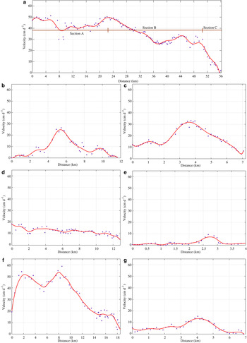
Fig. 7. Velocity patterns along profiles AA′ to GG′ for the period 11 Dec 2008–26 Jan 2009 (Fig. 6). The curves have been smoothed using a moving average filter with a span of five observations.
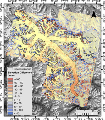
Fig. 8. Elevation difference map for Siachen Glacier for the period 1999–2007.
The mass budget of Siachen Glacier is computed to be −0.03 ± 0.21 m w.e. a−1 for 1999–2007 (Table 7) considering the density scenario 1 (uniform density) and −0.05 ± 0.18 m w.e. a−1 for the density scenario 2 (different densities in accumulation and ablation regions). Hence, the density scenarios hardly affect the result and indicate a more or less balanced mass budget.
5.4. Effect of debris cover
Debris constitutes a key component of a glacier system and affects the glacier in different ways. Usually thin debris enhances melt, while thick debris cover reduces melt (Nicholson and Benn, Reference Nicholson and Benn2006). Gardelle and others (Reference Gardelle, Berthier and Arnaud2012) reported that, on average, the elevation loss of exposed and debris-covered areas for the glaciers of the Eastern Karakoram are similar. To test this for Siachen Glacier, elevation differences over exposed and debris-covered ice were computed separately for lower elevation regions where debris-covered ice occurs (Fig. S1). However, it is important to note that exposed and debris-covered ice are dynamically coupled; hence, to observe possible subtle differences between the two, elevation changes in exposed and debris-covered regions have been classified into similar altitude intervals (Fig. 10). Here, we have randomly selected pixels over exposed and debris-covered ice such that the sampled pixels have similar frequency distribution with respect to their altitude. Thinning over debris-covered ice is slightly less than or comparable with that over exposed-ice areas for the same altitude range. One probable reason for this interesting observation is that debris-covered parts lying near the glacier margins have lower velocities compared with the exposed-ice parts located in the middle and having higher velocities (Fig. S2). In the lower ablation region (3600–4000 m), both exposed and debris-covered ice show strong thinning. In the elevation range 4000–4500 m, exposed ice shows equal or higher rates of thinning compared with debris-covered ice, although both rates are generally less than those below altitude of 4000 m. The thinning in the altitude band 4500–5000 m is smaller still, and debris-covered and clean ice show similar elevation changes. Among the debris-covered areas, the region between exposed ice and the debris-covered snout (with an elevation range of 3600–3700 m) demonstrates the highest thinning with a mean value of −30 m. One probable cause of the downwasting might be the presence of glacial lakes, which can be seen along the main trunk and along the lower western tributary glaciers. These lakes could, along with ice cliffs, enhance the ice melt at the debris-covered portions of the glacier (Ragettli and others, Reference Ragettli, Bolch and Pellicciotti2016).
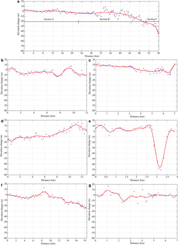
Fig. 9. Elevation changes along profiles AA′ to GG′ (Fig. 6). The curves have been smoothed using a moving average filter with a span of five observations.
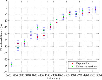
Fig. 10. Elevation changes over exposed and debris-covered ice as a function of altitude. Each elevation change has an uncertainty of ±2.0 m.
6. DISCUSSION
6.1. Elevation changes and velocity patterns
The average velocity for Siachen Glacier, 12.3 ± 0.4 cm d−1 during winter, is in close agreement with the average velocity of 13.7 cm d−1 reported by Copland and others (Reference Copland2009) for the nearby Baltoro Glacier for the period 26 July 2006–27 June 2007. Annual velocity estimates for other debris-covered glaciers such as Gangotri Glacier (Scherler and others, Reference Scherler, Bookhagen and Strecker2007; Bhattacharya and others, Reference Bhattacharya2016) and Khumbu Glacier (Quincey and others, Reference Quincey, Luckman and Benn2009; Bolch and others, Reference Bolch, Buchroithner, Peters, Baessler and Bajracharya2008) lie in the range 5.5–11 cm d−1, which is lower than the winter velocity of Siachen Glacier reported here. However, spatial heterogeneity needs to be taken into account when assessing how mass budget might affect velocity patterns and vice versa. Heid and Kääb (Reference Heid and Kääb2012) have shown that Siachen Glacier has negligible velocity changes in most of the lower ablation region, minor acceleration in its middle parts and large acceleration in its upper parts during the years 2000–08. Our study suggests that, in the upper ablation areas of the main trunk, climatic and topographic conditions resulted in high ice flux and insignificant elevation changes. However, low ice flux into the lower reaches of the ablation area is probably one reason for thinning. The region between snout and exposed-ice records thinning of 30 m for the period 1999–2007 and exhibit low velocity conditions. On the western tributary glaciers, profiles BB′, CC′, DD′, EE′ and GG′ (Fig. 6) showed significantly lower velocities than the average velocity of Siachen Glacier. These western tributary glaciers are characterized by an overall thinning and low velocities (Table 8). Profile FF′ (Figs 7f, 9f), located on the only western tributary glacier, which has velocities comparable with the average velocity of Siachen Glacier, shows elevation losses throughout its length. Profile DD′ shows elevation loss even in the accumulation regions and elevation gain in parts of the lower ablation zone. This is a hint for a recent surge of this tributary; tributary surges are quite common in the Karakoram (Belò and others, Reference Belò, Mayer, Smiraglia and Tamburini2008; Paul, Reference Paul2015). The velocity information from 2007 to 2008 for this tributary shows no abnormal behavior and hence indicates that the active phase of the possible surge was over by then.
6.2. Comparison of mass budget and area change estimates
The area of Siachen Glacier has not changed significantly since 1980. Similar results are obtained for the change in elevation of the glacier, which is equal to −0.23 ± 2.00 m for the 8 years between 1999 and 2007 or −0.03 ± 0.25 m a−1. Moderate thickening at high altitude is evidently balanced by significant thinning at lower altitude (Fig. 8). Moreover, for estimation of mass budget, we had considered two density scenarios, the results from which were indistinguishable. There exists only one other recent mass budget estimate for Siachen Glacier. Our estimate (−0.03 ± 0.21 m w.e. a−1) is roughly comparable with the +0.14 ± 0.14 m w.e. a−1 for the period 2000–08 reported by Gardelle and others (Reference Gardelle, Berthier, Arnaud and Kääb2013). However, their estimate did not include contributions from the lower portions of the ablation region, where we found significant elevation loss. On the other hand, some portions of the accumulation region, which are potentially gaining mass, are unaccounted for in the present study. It seems that the balanced mass budget of Siachen Glacier is not a recent phenomenon since Zaman and Liu (Reference Zaman and Liu2015) reported a mass budget with upper and lower bounds of +0.22 and −0.23 m w.e. a−1 during the period 1986–1991. The mass budget results computed by Zaman and Liu (Reference Zaman and Liu2015) using hydrological method with probable overestimation of mass loss due to evaporation seem to be consistent with results of this study. Our study shows that while the snout has been stable during the period 1980–2014, the transition between exposed and debris-covered ice advanced down-glacier between 1980 and 2007 and retreated rapidly up-glacier (by ~1.3 km) thereafter (2007–14). However the changes we describe above is in reference to the main trunk of Siachen Glacier only. Overall, exposed-ice area has decreased steadily, though slightly, over the period 1980–2014 (Table 5).
7. CONCLUSION
This study presents area change from 1980 to 2014 and mass budget from 1999 to 2007 of Siachen Glacier in the eastern Karakoram. The area of Siachen Glacier has shown no significant variations during the study period. However, the area of the exposed ice decreased steadily between 1980 and 2014. Also evident is the sudden drastic retreat (~1.3 km) of the distal part of the transition between exposed and debris-covered ice. This is likely to be caused by downwasting of ice in the lower ablation reaches near the terminus of the glacier. These observed changes are despite the fact that a near-zero mass budget for Siachen Glacier (−0.03 ± 0.21 m w.e. a−1) has been obtained for 1999–2007.
The average velocity of Siachen Glacier for December 2008–January 2009 is 12.3 ± 0.4 cm d−1. The velocity distribution for the main trunk of Siachen Glacier corresponds to that of a typical debris-covered glacier in the Himalayas, with low flow velocity at the head, increasing velocities in the upper accumulation area, almost constant velocities in the lower accumulation area and rapid decline towards velocities near zero near the terminus. The western tributary glaciers and lower ablation area of Siachen Glacier are sites of low ice flux. Debris-covered ice shows elevation losses comparable with those of exposed ice occurring at similar altitudinal ranges. The debris-covered ice located mainly near the margins of the glacier suffers from higher elevation losses. Thus, the spatial heterogeneity is an important component of the Siachen Glacier system and it should be analyzed in greater detail for future studies.
SUPPLEMENTARY MATERIAL
The supplementary material for this article can be found at https://doi.org/10.1017/jog.2016.127.
ACKNOWLEDGEMENTS
We would like to thank the European Space Agency for providing the Envisat data under the AOE 668 project. T. Bolch and T. Strozzi acknowledge funding by the European Space Agency (ESA) within the Glaciers_cci project (code 4000109873/14/I-NB).


 Open access