


1. Introduction
Ice streams are sections of ice sheets where the ice moves at substantially faster rates than the surrounding ice. As a result of the increased velocity, ice streams have a major impact on the rate of discharge and mass balance of an ice sheet (Bamber and others, Reference Bamber, Vaughan and Joughin2000; Livingstone and others, Reference Livingstone2012). Therefore, modern ice streams have been studied in detail and mapping of former ice streams has led to a better understanding of their processes (Stokes, Reference Stokes2018). The Oneida Ice Stream was a major ice stream of the Laurentide Ice Sheet (LIS) that developed between modern Lake Ontario and Oneida Lake at the end of the Pleistocene (Briner, Reference Briner2007; Hess and Briner, Reference Hess and Briner2009) (Fig. 1), and was part of the Oneida Lobe, a sub-lobe of the Ontario Lobe (Fig. 1a). The Oneida Ice Stream as well as many of the ice streams of the LIS were identified by studies of light detection and ranging (LIDAR) data and high-resolution digital elevation models that reveal glacial bedforms indicative of faster flow (Fig. 1b) (Briner, Reference Briner2007; Hess and Briner, Reference Hess and Briner2009; Sookhan and others, Reference Sookhan, Eyles and Putkinen2018). These bedforms include drumlins and megascale glacial lineations (MSGLs) observed west of the Oneida Basin (Briner, Reference Briner2007; Murari and others, Reference Murari, Domack and Owen2016; Sookhan and others, Reference Sookhan, Eyles and Putkinen2018). The Oneida Basin was subsequently infilled by proglacial and Holocene lacustrine sediments (Zaremba and Scholz, Reference Zaremba and Scholz2021), and therefore LIDAR data cannot provide information on the deglaciation of this basin. To fully assess the development and extent of the Oneida Ice Stream, a subsurface investigation of Oneida Lake is required. Ice stream formation and ice flow velocities are dependent on many factors including basal drag, regional topography and roughness of the underlying surface (Price and others, Reference Price, Conway, Waddington and Binschadler2008; Haseloff and others, Reference Haseloff, Schoof and Gagliardini2015; Schoof and Mantelli, Reference Schoof and Mantelli2020). Basal drag can be decreased by the presence of meltwater between the ice sheet and the underlying surface (Price and others, Reference Price2017) while topographic lows can focus ice flow increasing the velocity (Haseloff and others, Reference Haseloff, Schoof and Gagliardini2015; Schoof and Mantelli, Reference Schoof and Mantelli2020). Sediment-filled, deep-water bodies such as a proglacial lake have been shown to accelerate ice velocities (Geirsdóttir and others, Reference Geirsdóttir, Miller, Wattrus, Bjömsson and Thors2008). Ice streams are initiated at ice margins and pull ice from the ice-sheet interior (Price and others, Reference Price, Conway, Waddington and Binschadler2008). The depth to top of Paleozoic strata provides the best estimate of the regional topography during deglaciation within the Oneida Basin (Zaremba and Scholz, Reference Zaremba and Scholz2021). Therefore, constraints on the depth to the top of Paleozoic strata contribute to understanding the formation and evolution of the Oneida Ice Stream. Previous studies interpreted that paleo–ice flow velocities of the Oneida Ice Stream were relatively high on the western coast of the lake (Briner, Reference Briner2007; Hess and Briner, Reference Hess and Briner2009). Here we address the possibility that the Oneida Basin influenced the development of the Oneida Ice Stream by providing a topographic low that focused ice flow and increased ice velocities (Haseloff and others, Reference Haseloff, Schoof and Gagliardini2015; Schoof and Mantelli, Reference Schoof and Mantelli2020). The majority of fill in the Oneida Basin consists of proglacial lake and Holocene sediments overlying Paleozoic strata (Zaremba and Scholz, Reference Zaremba and Scholz2021). Determining the depth to the top of the Paleozoic strata provides estimates on the depth of the proglacial lake, topography during deglaciation and depth of a calving margin in the basin. While not mutually exclusive to ice streaming, the presence of a calving margin would provide an additional mechanism that could have accelerated mass loss from the ice sheet and alter deglaciation of the area.

Fig. 1. (a) Greater Lake Ontario basin with location of the Oneida Lobe of the Laurentide Ice sheet as well as extent of Glacial Lake Iroquois. The shapefiles for the location of the LIS margins are from Franzi and others (Reference Franzi2016). The shoreline of Glacial Lake Iroquois is from Bird and Kozlowski (Reference Bird and Kozlowski2016). (b) Oneida Lake and a section of the New York Drumlin field with the location of the Oneida Ice Stream labeled. The shapefile of the delineated subglacial bedforms (e.g. drumlins) is from Hess and Briner (Reference Hess and Briner2009).
The Oneida Basin is potentially an important paleoclimate reference site in North America, in addition to contributing to the understanding of glacial landforms and ice streams in the region. Ice-sheet processes such as ice discharge rates and punctuated drainages of proglacial lakes are documented to affect Northern Hemisphere climate (Broecker and others, Reference Broecker1989; MacAyeal, Reference MacAyeal1993; Broecker, Reference Broecker1994; McCabe and Clark, Reference McCabe and Clark1998). The Oneida Basin was occupied by Glacial Lake Iroquois, a large and deep proglacial lake that experienced high rates of sedimentation (Murari and others, Reference Murari, Domack and Owen2016; Zaremba and Scholz, Reference Zaremba and Scholz2021) (Fig. 1a). The proglacial lake deposits in Oneida Lake likely contain a paleoclimate record of Ontario Lobe meltwater fluctuations that spans multiple abrupt cold stadials that occurred at the end of the Pleistocene (Ridge and others, Reference Ridge2012; Franzi and others, Reference Franzi2016; Zaremba and Scholz, Reference Zaremba and Scholz2019, Reference Zaremba and Scholz2021) (Fig. 1). Comparing records of Ontario Lobe meltwater production with Greenland Ice Sheet records can help better constrain the connection between the LIS deglaciation and North Atlantic climate, as was completed for LIS lobes east of the Ontario Lobe (Ridge and others, Reference Ridge2012).
Previous studies attempted to assess the depth to the top of Paleozoic strata or thickness of the Quaternary deposits in the Oneida Basin using multichannel seismic (MCS) reflection data (Zaremba and Scholz, Reference Zaremba and Scholz2021). While the methodology proved successful, two issues prevented a thorough evaluation of the basin. Glacial deposits such as drumlins or moraines contain boulders and other large clasts (Hanvey, Reference Hanvey1991; Stokes and others, Reference Stokes, Spagnolo and Clark2011) that create numerous point reflections which reduce the continuity of stratal reflections. This can reduce the fidelity of the data below the point reflectors and create areas where the depths to top of Paleozoic strata are ambiguous. This makes interpreting the depth to the top of Paleozoic strata difficult and is compounded by the lack of coherent reflections below the top of Paleozoic strata in the reflection dataset (Zaremba and Scholz, Reference Zaremba and Scholz2021).
A more universal issue common with late-Quaternary or Holocene studies is the attenuation of the reflection signals from subsurface biogenic gas produced within pore spaces via the breakdown of Holocene organic matter (Anderson and Hampton, Reference Anderson and Hampton1980; Anderson and Bryant, Reference Anderson and Bryant1990; Hart and Hamilton, Reference Hart and Hamilton1993; Figueiredo and others, Reference Figueiredo, Nittrouer and de Alencar Costa1996; Missiaen and others, Reference Missiaen, Murphy, Loncke and Henriet2002; Dondurur and others, Reference Dondurur, Çifçi, Göktuğ Drahor and Coşkun2011; Zaremba and others, Reference Zaremba2016; Zaremba and Scholz, Reference Zaremba and Scholz2021). In the Oneida Lake seismic reflection data sets, the attenuation of the signal from biogenic gas occurs only in the deepest section of the modern lake, and where the Holocene section is thickest. It is also likely that the depth to top of Paleozoic strata is deepest in the sections attenuated by biogenic gas (Zaremba and Scholz, Reference Zaremba and Scholz2019, Reference Zaremba and Scholz2021). The thickest deposits within a basin are predominantly aligned with available accommodation space. In the Oneida Basin, the sections of the basin attenuated by biogenic gas represent a small area of the basin, however these are important sites for understanding the extent of the paleoclimate record contained within the lake as well as for understanding the deglaciation of the area. There is potential global application for a method that can provide insight into the subsurface in sections where seismic reflection datasets are attenuated by biogenic gas.
In this paper we apply first arrival seismic tomography methods to a dataset that was originally collected for MCS reflection imaging (Fig. 2) (Zaremba and Scholz, Reference Zaremba and Scholz2021). The methodology provides estimates into the depth to top of Paleozoic strata in areas where the MCS data failed to provide information. First arrival seismic tomography methods use the velocity of refracted P-waves to estimate a subsurface velocity model. Paleozoic strata in the Oneida Basin are overlain by unconsolidated Quaternary sediments, primarily proglacial lake deposits (Zaremba and Scholz, Reference Zaremba and Scholz2021). Head waves within the dataset with velocities of ~4000 m s−1 are likely the result of the seismic wave traveling within the Paleozoic strata. A subsurface velocity model created with the first arrival seismic technique informs on the depth to Paleozoic strata in the Oneida Basin. The intent of the tomography-derived velocity models was to independently confirm results from seismic reflection data, as well as provide information on the depth to basement in areas where reflection data failed to image the subsurface stratigraphy.

Fig. 2. Tracklines of 2D seismic reflection data with profiles analyzed for refraction tomography are indicated in red. The location of the subglacial bedforms (e.g. drumlins) from Hess and Briner (Reference Hess and Briner2009) is presented on the map. Elevation is in meters above mean sea level (mamsl).
2. Geology
Oneida Lake provides an excellent opportunity to utilize seismic reflection survey data to produce first arrival tomography-derived velocity models (Fig. 2). The lake contains a thick sequence of unconsolidated Quaternary deposits overlying the Paleozoic strata or sub-till eroded surface (Zaremba and Scholz, Reference Zaremba and Scholz2019, Reference Zaremba and Scholz2021). The Quaternary deposits consist primarily of proglacial lake deposits but also subglacial deposits including drumlins and various types of moraines (Zaremba and Scholz, Reference Zaremba and Scholz2021). Moraines and drumlins commonly contain cobbles and boulders (Hanvey, Reference Hanvey1991; Stokes and others, Reference Stokes, Spagnolo and Clark2011) which are likely responsible for the observed point reflections in the reflection profiles. Wells drilled on the south, east and north shore of the lake penetrate Paleozoic strata of the Clinton Group, Lockport Group, and Grimsby Formation (New York State Museum, 2021). Individual units within these groups and formation include sandstones such as the Grimsby and Herkimer Sandstone as well as shales, dolostones and limestones such as the Lakeport Limestone or Lockport Dolomite. Previous studies indicated that the Grimsby Sandstone has a seismic velocity of ~3.3–4 km s−1 and the Lockport Dolomite has velocities as high as 5.6 km s−1 (Engelder, Reference Engelder1979). In addition, velocities as high as 5.5 km s−1 in limestones and as low as 3.5 km s−1 in shales are observed in Paleozoic strata such as the Marcellus shale found within the area (Zhu, Reference Zhu2013). The wells indicate Paleozoic strata are ~700 m thick and overlie Precambrian granites, much deeper than the depth of investigation in this study (New York State Museum, 2021). From the depth-converted reflection seismic data, the maximum dip of the incised bedrock units in the Oneida Basin is estimated to be ~3°, although most observations are of dips of 1–2°.
3. Methods
3.1. Multichannel seismic data acquisition
In July of 2019 ~217 km of 2D MCS reflection data were collected along 27 profiles within Oneida Lake (Fig. 2; Figs S1, S2). A 120 channel Seamux™ solid-towed array marine streamer with a 3.125 m channel group interval was used for channels 1–120 and for channels 121–144 an interval of 6.25 m was used. This produced a maximum offset of ~540 m. A 4 × 10 in3 Bolt 2800 LLX airgun array was used as the seismic source (Fig. 3). The air gun array was towed at ~1 m depth to allow for venting of seismic source air bubbles and was fired every 6.25 m using positioning control from two Trimble GPS receivers with sub-meter accuracy. Seismic record length was 2 s and the sample rate for each seismic trace was 0.25 ms. Seismic lines varied in length from 5 to 9 km with ~1000 shots per line. Accordingly, the distance from the hydrophones to the seismic source remained constant, unlike most first arrival seismic tomography or refraction surveys where the hydrophones/geophones remain in place and the active seismic source is repositioned (Toomey and others, Reference Toomey, Solomon and Purdy1994; Göktürkler, Reference Göktürkler2009). This dataset does not contain reversed shots, as seismic reflection surveys are only shot in one direction.

Fig. 3. (a) Shot gather from line MCS-06. (b) Shot gather with the location of first arrivals highlighted in red. Refracted arrival has an estimated velocity of ~4500 m s−1. Other refractions observed within line MCS-06 shot gathers indicate velocities as high as 5000 m s−1 and as low as 3500 m s−1. Though this is not depicted in the shot gather there is a change in the channel interval; channels 1–120 are spaced at 3.125 m while channels 121–144 are spaced at 6.25 m.
3.2. Data conditioning
First arrival times were picked and data modeled to determine the subsurface velocities using Geogiggas DW TOMO™ codes. DW TOMO is commonly used in the geophysical community (Glas and others, Reference Glas2019; Claes and others, Reference Claes, Paige, Gordon, Parsekian and Miller2021; Huang and others, Reference Huang2021). Geogiga's DW TOMO begins with an initial velocity model and iteratively performs inversions reducing the model's misfit to the observed arrival time. An iterative approach is required because of the inherent nonlinearity in this inverse problem. The travel times of the first arrivals remain constant while the wave paths are altered by the velocity structure created in the iterative process. First arrivals consisted of direct arrivals and head waves. Shot gathers in SEGY format were imported into Geogiga DW TOMO in ten shot increments with spacings of ~62.5 m (Fig. 3). This provided a spatially-dense dataset for every line, with overlapping ray paths. This code uses ray tracing or shortest path method in the forward modeling process (Moser, Reference Moser1991). The forward model or initial velocity model is a subsurface velocity model defined by the user. The intent of the tomography-derived velocity models was to independently confirm results from seismic reflection data, as well as provide information on the depth to basement in areas where reflection data failed to image the subsurface stratigraphy. Therefore, a priori data from the reflection dataset were limited in the tomography inversion process. The initial model contained a surface velocity of 1350 m s−1 and increased to 1600 m s−1 over a depth of 15 m. Below 15 m the model increased by 390 m s−1 every 1 m to reach a velocity of 5500 m at 25 m depth. The velocities used in the model were derived from MCS reflection data collected within the basin that provided estimates on the velocity of the Quaternary deposits (Zaremba and Scholz, Reference Zaremba and Scholz2021). A relatively high maximum velocity of 5500 m s−1 was used based on apparent maximum velocities of ~5000 m s−1 obtained from refractions. However, it should be noted these are apparent velocities on account of dipping surfaces. Paleozoic stratigraphic units that have also been identified near the lake have velocities of ~3300–5500 m s−1 (Engelder, Reference Engelder1979; Zhu, Reference Zhu2013).
The selection of the maximum velocity is an important constraint, as it limits the final model maximum velocity. Therefore, the maximum velocity used is high to ensure the final output is not limited by the initial model. Similarly, a value of 1350 m s−1 was used as the minimum velocity. This value was decided upon to account for the possibility of gas in fine-grained sediment pores which could reduce the velocity that a seismic wave travels through the subsurface (Ghosh and Sain, Reference Ghosh and Sain2008). Multiple distinct initial models were used before the final starting model was selected. The depths to maximum velocity were altered in the various forward models with little effect on the results. However, artifacts from the forward model were observed in the final output if the depth to maximum velocity was set significantly deeper than the refracting surface. Therefore, a depth of 25 m was established for the depth of the maximum velocity to reduce the effects of the forward model on the output. The same forward model was used for every line, and each line was subjected to nine iterations with a maximum disturbance of 75%. The inversion process uses an algorithm adapted from Toomey and others (Reference Toomey, Solomon and Purdy1994), which accounts for previous knowledge such as the prior iteration, smoothing parameters, and travel time uncertainties which are established by the user. Following careful parameter testing, the smoothing parameters chosen for use in the algorithm were 3.75 m for the vertical smoothing, 15.5 m for the horizontal smoothing and a picking uncertainty of 1 ms (Fig. S3). All of the tomography-derived velocity models included in this paper are available for download at the Marine Geosciences Data System (Zaremba and Scholz, Reference Zaremba and Scholz2022).
3.3. Test dataset
Lines MCS-06 and MCS-04 were chosen as test datasets in this study (Figs 4–6). These lines were chosen as the best calibration lines because they contained a continuous, high amplitude, reflection interpreted to be the top of Paleozoic strata in the reflection dataset. These interpretations could be made with a high degree of confidence in the MCS reflection dataset in line MCS-06 and MCS-04. In addition, the depths to the top of Paleozoic strata for MCS-06 and MCS-04 indicate considerable variation in relief. Therefore, these lines provided a range of dips and depths to the top of the Paleozoic strata essential for a robust test of this methodology. The other lines used in this study were chosen because they do not clearly image the top of Paleozoic strata on account of either attenuation of the reflection data from: (1) biogenic gas or (2) point reflections (Figs 7, 8). In addition, these lines contained shots with high-amplitude refracted arrivals, which decreased the uncertainty of picking the first arrivals, reducing the need for severe filtering, and enabling more consistent first-arrival picks throughout the dataset.

Fig. 4. (a) Velocity model produced by first arrival tomography for line MCS-06. (b) Velocity model produced by first arrival tomography with ray path coverage.

Fig. 5. (a) Line MCS-06 with the tomography velocity model overlain on top of the depth-converted reflection data. (b) The iso-velocity contour of 3650 m s−1 is highlighted in red. This line follows the interpreted top of the Paleozoic strata reflection surface.

Fig. 6. (a) Line MCS-04 with the tomography velocity model overlain on top of the depth-converted seismic reflection data. (b) The iso-velocity contour of 3650 m s−1 is highlighted in red. This line follows the interpreted top of the Paleozoic strata reflection surface.

Fig. 7. (a) Line MCS-25 with the tomography velocity model overlain on top of the depth converted seismic reflection data. (b) The iso-velocity contour of 3650 m s−1 is highlighted in red. This line follows the interpreted depth to the top of Paleozoic strata. The iso-velocity line also defines the base of a drumlin, consistent with previous interpretations on the depth to the top of Paleozoic strata.
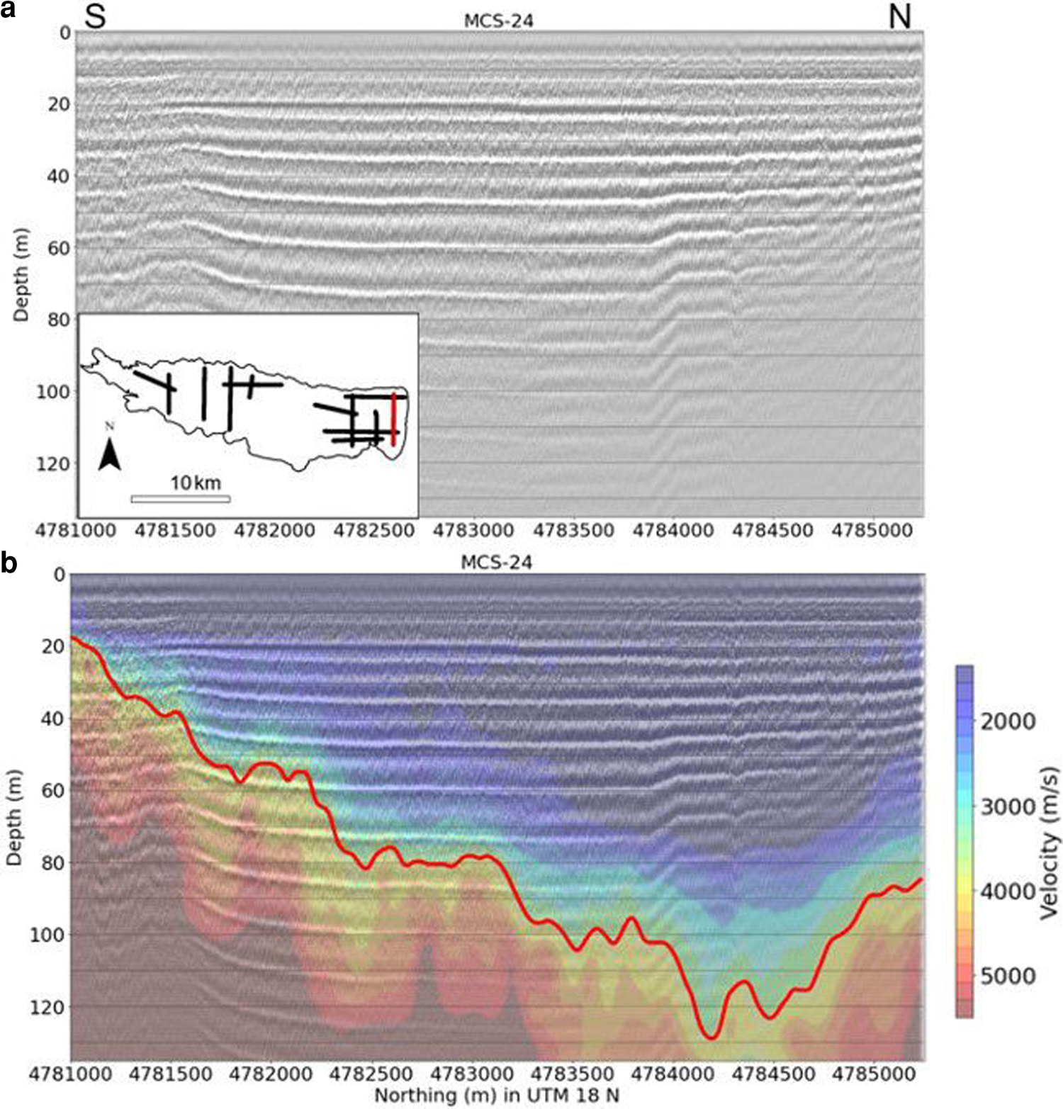
Fig. 8. (a) Reflection profile MCS-24 attenuated by biogenic gas, and therefore providing limited subsurface information. (b) The tomography velocity model and iso-velocity contour of 3650 m s−1 highlighted in red provides an estimate of the depth to the top of Paleozoic strata.
3.4. Seismic reflection data
The following processing steps were applied to the reflection dataset using Landmark SeisSpace/ProMAX™ software. Geometry was applied using source and receiver offsets with group and shot intervals, and data were sorted into the common midpoint (CMP) domain. For the reflection dataset, only the first 120 channels were used to maintain a consistent channel group interval of 3.125 m. Stacking velocities were picked using a combination of velocity semblance plots and constant velocity stacks applied to CMP supergathers. For the constant velocity stacks, supergathers were constructed from 51 CMPs and analyzed in increments of 100 CMPs. After time–velocity pairs were selected, normal moveout was applied, and the data were stacked. Nested Ormsby band-pass filters of 110–135–1500–1700 Hz and 40–70–1100–1300 Hz were applied to the stacked datasets. Ormsby filter frequencies were picked by executing a careful parameter test whereby frequencies were altered incrementally until the ideal filter was produced. The ideal filter was selected based on a qualitative viewing of the data. This filter enhanced images of both the high-frequency reflections of the proglacial material and the higher amplitude reflections that delineate the glacial till and Paleozoic strata. A post-stack F-K filter was applied to remove steeply dipping noise, and a careful comparison of F-K filtered profiles and raw profiles was conducted. A post-stack Kirchhoff time migration with a 200 ms bottom taper was applied using the root mean square stacking velocities picked for each seismic profile. MCS data included in this paper are available for download at the Marine Geosciences Data System (Scholz and Zaremba, Reference Scholz and Zaremba2022).
Conversion of the reflection seismic data from two-way travel time (twtt) to depth in meters was conducted using Landmark SeisSpace/ProMAX™. This required the conversion of the stacking velocities to interval velocities. The interval velocities were then used to depth convert the seismic profiles from the time domain to depth domain.
3.5. Comparison of tomography-derived velocity structures and multichannel reflection seismic data profiles
The tomography-derived velocity models were compared to the depth converted reflection profiles to validate the first-arrival tomography approach. The tomography-derived velocity models were overlain on the depth-converted reflection profiles (Figs 4–6) allowing for a qualitative comparison of the two datasets. In addition, the interpreted depth to Paleozoic strata horizons was exported from Landmark DecisionSpace™ and plotted with iso-velocity contours exported from the tomography-derived velocity models (Fig. 9). This provided a more precise assessment of the two datasets and allowed for selection of appropriate iso-velocity contours that would best represent the top of Paleozoic strata (Fig. 9).

Fig. 9. (a) Profile MCS-06: plot of interpreted depth to top of Paleozoic strata from reflection data in yellow vs tomography velocity iso-velocity contour of 3650 m s−1 in red and 4200 m s−1 in blue. (b) Profile MCS-04: plot of interpreted depth to top of Paleozoic strata from reflection data in yellow vs tomography velocity iso-velocity contour of 3650 m s−1 in red and 4200 m s−1 in blue.
4. Results
4.1. First arrivals
First arrivals were easily identified with low uncertainty due to the high fidelity of the streamer data. The first arrivals were picked on the direct arrival which has a velocity of ~1450 m s−1 as well as high velocity refractions (Fig. 3). The majority of the higher velocity refractions were ~4000 ± 800 m s−1 with rare refractions as high as 5000 m s−1. In a few instances additional refractions with velocities of ~2000 ± 200 m s−1 were observed arriving later than the high velocity refraction; however, these refractions were not picked. None of the velocities reported above were corrected for dip and are reported as they were observed in the shot gathers.
4.2. Fitting errors of the tomography data
Generally, shot spacing and channel intervals provided significant overlap of ray paths. Average root-mean-square fitting values of the observed data and tomography-derived velocity models for the 12 lines processed in this study varied between 0.5 and 1 ms. Average fitting errors were higher at the edges of lines as ray path coverage was reduced in these areas.
4.3. Tomography-derived velocity models
Interpretations of the tomography-derived velocity models were limited to areas with high ray path coverage (Fig. 4b). Velocities higher than 4500 m s−1 had poor ray path coverage and were likely an artifact of the initial model and therefore, were not considered as reliable. Internal consistency among the tomography-derived velocity models can be confirmed by analysis of intersecting velocity models as illustrated by the fence diagrams (Figs 10, 11). The depth to iso-velocity contours of intersecting or adjacent profiles are similar, even when the selected profiles were variably oriented to regional dip.

Fig. 10. (a) Fence diagram of tomography-derived velocity profiles for MCS-08, MCS-06 and MCS-25. Viewpoint is from the south-west looking north-east. (b) Fence diagram of tomography-derived velocity profiles for MCS-08, MCS-06 and MCS-25. Viewpoint is from the north-east looking south-west. Note the internal consistency of the velocity models with depth.

Fig. 11. (a) Fence diagram of tomography-derived velocity profiles for MCS-20, MCS-13, MCS-22 and MCS-19D. Viewpoint is from the south-west looking north-east. (b) Fence diagram of tomography-derived velocity profiles for MCS-20, MCS-13, MCS-22 and MCS-19D. Viewpoint is from the north-west looking south-west. Note the internal consistency of the velocity models with depth.
4.4. Comparison of reflection data and tomography-derived velocities
Initial comparison of the depth-converted seismic reflection data and tomography-derived velocity models indicates that the interpreted top of Paleozoic strata reflection coincides with a velocity of ~3650–4200 m s−1 (Fig. 9). The reflection-derived interpreted depth to Paleozoic strata and the iso-velocity contour line of ~3650 m s−1 covary. It should be noted that a faster iso-velocity contour line of up to 4200 m s−1 covaries with the depth to top of Paleozoic strata as well (Fig. 9), however, ray path coverage of the slower velocities is better, and therefore provides more reliable interpretations. Use of the slower iso-velocity contour provides a minimum depth to the Paleozoic strata and is therefore a more conservative estimate.
5. Discussion
5.1. Methodology successes and limitations
The first arrival seismic tomography method using unidirectional refraction data has been explored in the marine offshore environment where the use of long streamers of several kilometers length is possible (Zelt and others, Reference Zelt2004; Ehrhardt and Schnabel, Reference Ehrhardt and Schnabel2019; Ghosal and Singh, Reference Ghosal and Singh2021). However, the methodology has been underutilized on smaller scales onshore or in lacustrine Quaternary studies. The results from this study suggest that the methodology is promising and should be explored and developed more extensively for other shallow Quaternary investigations, and especially studies investigating glaciated basins or proglacial lakes. However, further refinement of the method is beyond the scope of this paper, which aims to extend previous analyses of MCS data and provides estimates on the depth to the Paleozoic strata in sections of a basin where reflection seismic data provide limited information.
Even though ray path coverage is dense within the Quaternary section of the tomography-derived velocity models, this section of data should be interpreted carefully. The first arrivals picked in the dataset consisted of direct arrivals traveling through the water column and high velocity refractions interpreted to be primarily from the surface of Paleozoic sedimentary rocks. The refraction arrivals and tomography-derived velocity models constrain the depth to the high velocity layer, interpreted as the top of Paleozoic, and do not provide information on velocities or features within the Quaternary section. It is likely that velocity variations within the Quaternary section of the tomography-derived velocity models are a result of smoothing during the inversion process. Furthermore, the reflection seismic data failed to image any structures below the high-amplitude reflection interpreted as the top of Paleozoic strata. Accordingly, information on the velocity of the Paleozoic strata or anything below it is absent for the reflection dataset. For these reasons, direct comparisons of the tomography-derived velocity models and reflection seismic interval velocity data are of limited utility as they provide information on different sections of the basin.
Iso-velocity contours of ~3650–4200 m s−1 covary with the reflection interpretations for depth to the top of the Paleozoic strata in the test dataset which consists of lines MCS-06 and MCS-04 (Fig. 9). Therefore, the tomography-derived velocity models can provide insight into the depth to the Paleozoic strata in sections of the basin where reflection data provide little to no information. The choice of an iso-velocity contour of 3650 m s−1 provides the best estimate for depth to top of Paleozoic strata. A faster velocity would provide similar results, however localized unrealistic velocity structures occur when a faster iso-velocity contour is used (Fig. 9). In addition, ray path coverage of the slower iso-velocity contour of 3650 m s−1 is more consistent for the entire dataset and therefore provides a more reliable estimate of depth to top of Paleozoic strata. A velocity of 3650 m s−1 is too fast to be till as velocities ranging from 1500 to 2700 m s−1 are often reported for tills (Aziman and others, Reference Aziman, Hazreek, Azhar and Haimi2016).
The tomography-derived velocity models are internally consistent, suggesting the method is reliable. This is apparent in the fence diagrams that show intersecting tomography velocity models with the same changes in velocity with depth (Figs 10, 11). Notably, these lines were all collected at different orientations to the prevailing dip direction of the top of Paleozoic strata/sub-till eroded surface, and arrive at similar results. This robust result indicates that the lack of reverse shots is mitigated by the high data density utilized in the analyses.
The success of this method relies heavily on the high spatial data density of the marine (streamer) seismic reflection survey, as well as the long offsets relative to depth of investigation (Figs 3, 9). In addition, the geology of the basin is well suited for this methodology. A priori data indicate that thick unconsolidated Quaternary deposits overlie consolidated Paleozoic strata. Therefore, the basin has a high contrast in velocities between the top of Paleozoic strata and the Quaternary fill. In addition, the maximum observed dips of the top of Paleozoic strata are ~3° in the basin, with the majority much less, reducing the effect of dip on the apparent velocity of the refractions. Other glacially-incised basins or lakes are good candidates for this method as glacial processes tend to erode preexisting materials and deposit large amounts of sediments on recently eroded bedrock surfaces within short time periods. This provides a strong velocity contrast with overlying glacial deposits.
5.2. Insights into the deglaciation of the Oneida Lake region and ice stream formation
First arrival seismic tomography provides new insights into the depth and geometry of the top of the Paleozoic strata in the study area (Figs 8, 12). Previous work using reflection seismic data estimated the maximum depth to the top of the Paleozoic strata surface to be ~90 m below lake surface (Zaremba and Scholz, Reference Zaremba and Scholz2021). However, use of the first arrival seismic tomography technique improves this estimate, provides evidence that the maximum depth to this surface is ~125 m below modern lake surface (modern lake level is 112 m above sea level) or 13 m below sea level, and constrains the morphology of the depth to top of Paleozoic strata (Fig. 8). This indicates ~108 m of Quaternary sediments are present in the deepest section of the basin. It is important to note that this additional 35 m is not a result of a discrepancy between the two methods. The reflection data and tomography-derived velocity models generate similar results where data coverage is available for both techniques. The reflection dataset did not image the deepest section of the basin everywhere because of attenuation of the signal likely from biogenic gas in Holocene sediment pore spaces (Fig. 8a). The depth to the top of the Paleozoic strata from the tomography-derived velocity models, as well as previous work which identified Glacial Lake Iroquois shorelines ~35 m above the modern lake surface, suggest a ~160 m deep proglacial lake was present in the basin (Fairchild, Reference Fairchild1909; Fullerton, Reference Fullerton1980; Franzi and others, Reference Franzi2016). However, this estimate is based on Glacial Lake Iroquois shorelines and is likely an underestimate for proto-Iroquois lakes which were known to have shorelines at higher elevations (Fairchild, Reference Fairchild1909; Fullerton, Reference Fullerton1980; Franzi and others, Reference Franzi2016). In addition, this dataset suggests that the basin becomes wider in the eastern section of the lake than previously thought, ~4–5 km across (Fig. 12).

Fig. 12. Depth to top of the Paleozoic strata from the combination of reflection seismic data and tomography velocity models.
The increase in depth and width of this basin is significant given the results of prior research. Previous work identified drumlins and MSGLs within the western section of the Oneida Basin (Zaremba and Scholz, Reference Zaremba and Scholz2021). The drumlins and MSGLs were interpreted to be an extension of the elongated drumlins observed west of the lake that are indicative of fast ice flow velocities and provide evidence of the Oneida Ice Stream (Briner, Reference Briner2007; Hess and Briner, Reference Hess and Briner2009). The occurrence of these bedforms and orientation of the basin's axis aligned in the direction of the Oneida Ice Stream's flow provide compelling evidence that ice stream processes occurred within the western section of the basin (Briner, Reference Briner2007; Hess and Briner, Reference Hess and Briner2009; Zaremba and Scholz, Reference Zaremba and Scholz2021). The identification of the Oneida Basin in this study adds to the interpretation that elongated drumlins observed to the west and north of the study are a result of the Oneida Ice Stream, as the basin provides a topographic low which promoted and steered the ice stream (Haseloff and others, Reference Haseloff, Schoof and Gagliardini2015; Schoof and Mantelli, Reference Schoof and Mantelli2020). The change in gradient as well as wet-based conditions that would have been present while the ice sheet retreated from the Oneida Basin would have increased ice flow velocities. Therefore, the presence of this deep basin should be considered in evaluating the deglaciation of the area, as this topographic low could have aided in ice stream formation at various stages of deglaciation.
Other glacial landforms such as De Geer moraines buried by proglacial lake deposits have been identified in the basin (Zaremba and Scholz, Reference Zaremba and Scholz2021). This provides evidence that a calving margin occupied the basin during retreat of the ice sheet, sometime after ~14.8 kyr BP (Lindén and Möller, Reference Lindén and Möller2005; Franzi and others, Reference Franzi2016). Ice streams initiate at ice margins and therefore ‘pull’ ice from the interior of an ice stream (Price and others, Reference Price, Conway, Waddington and Binschadler2008). The presence of bedforms such as De Geer moraines that indicate calving processes support the interpretation that the deep, water-filled basin affected ice flow velocities (Zaremba and Scholz, Reference Zaremba and Scholz2021). However, it is difficult to discern the extent to which this would affect ice flows and if it was responsible for the formation of the ice stream. East of the basin within the Mohawk Valley there is little evidence for another topographic low that could have impacted ice velocity as much as the Oneida Basin (Fig. 13). The deeper and wider basin identified in this study by the tomography-derived velocity models would have floated more ice or destabilized a larger section of the ice-sheet base, which would have allowed calving of a thicker ice sheet. The increased gradient and wet-based conditions of the basin and calving processes aid in explaining why drumlins and MSGL are more common west of the lake, as well as the presence of elongated drumlins near the western shoreline of Oneida Lake. There is much less evidence of Oneida Lobe ice streaming processes east of the lake (Hess and Briner, Reference Hess and Briner2009; Sookhan and others, Reference Sookhan, Eyles, Bukhari and Paulen2021).

Fig. 13. Three-dimensional perspective of the Oneida Basin viewed east toward the Mohawk Valley, in the direction of ice flow as well as the drainage direction of Glacial Lake Iroquois. Within Oneida Lake the surface is the top of the Paleozoic strata, with the water column and Quaternary sediment column stripped away. Within the lake, depth-converted seismic reflection profiles and tomography velocity models are shown with the top of Paleozoic strata surface. The top-Paleozoic surface within Oneida Lake was generated from data presented herein. The surrounding catchment is a 1 arc second (~30 m) digital elevation model.
The Oneida Basin was not the only influence on the formation of the Oneida Ice Stream, nor did the basin initiate the ice stream. Drumlins to the south of the lake indicate that the ice stream operated across a part of the valley wider than what was occupied by the lake (Briner, Reference Briner2007; Hess and Briner, Reference Hess and Briner2009). However, a deep and wide proglacial lake with bedforms indicative of calving processes very likely exerted considerable effect on ice velocities, and was important for the Oneida Ice Stream development and in the deglaciation of the region. Ice recession rates in the region likely increased because of calving processes, as occurred in the Champlain lowlands (Franzi and others, Reference Franzi2016). Drumlins can form very rapidly and abruptly (King and others, Reference King, Woodward and Smith2007; Dowling and others, Reference Dowling, Möller and Spagnolo2016) and therefore could be a result of a short-lived increase in ice flow velocities. The drumlins identified south of the lake could have formed at a different time than those observed west of the lake and are possibly the result of a different flow regime of the Oneida Ice Stream. The drumlins observed west of the lake may reflect the latest stages of the ice stream when it was affected by the Oneida Basin and may not be indicative of ice stream velocity over its entire duration. The exact timing of ice streaming in the area is poorly constrained. However, even if the calving margin developed after ice streaming ceased it still likely had a major impact on the deglaciation of the area, as calving margins can significantly increase ice flow velocities and mass loss from an ice sheet. Observations from the modern Greenland Ice sheet indicate that calving events can lead to ~30% increases in ice flow velocities and increased mass loss from an ice sheet (Thomas, Reference Thomas2004). Therefore, even if the calving margin was only active after ice stream processes ceased, the discovery of this basin still has major implications for understanding the deglaciation of the basin.
The topographic low and presence of a calving margin in the eastern end of the Oneida Basin helped determine the location of the ice stream and provides evidence for a mechanism to increase ice flow. Topographic lows and associated paleo-ice streams are interpreted for the Finger Lakes to the west, where bedrock topography affected the location of ice stream flowlines and where a water-terminating ice margin triggered fast ice flow that altered pre-existing bedforms (Sookhan and others, Reference Sookhan, Eyles, Bukhari and Paulen2021). This Oneida Lake study suggests that more detailed analyses of paleo-ice streams are required in order to better understand their processes and that, subsurface data investigations should be considered when reconstructing paleo-ice streams. The basin discovered in this study impacted ice velocities west of the lake either by facilitating the formation of the Oneida Ice Stream or even by the development of a calving margin alone. It also provides evidence of a basin of more than 125 m depth which could have allowed for a later pulse of ice streaming. This study suggests that the history of the Oneida Ice Stream might be more complicated than originally thought and the bedforms we observe today could be the result of multiple ice stream pulses or multiple ice streaming events.
The wide eastern section of the basin may be a consequence of several factors, including possible enhanced bedrock erodibility, pronounced glacial/fluvial erosion or fluvial knickpoint migration (Fig. 12). The more extensive and refined estimates of the depth to top of the Paleozoic strata surface presented herein (Fig. 12) also suggest that the Oneida Basin was likely the result of glacial erosion and not the result of another mechanism such as fluvial incision. This conclusion is based on the geometry and orientation of the basin's axis, as the basin shallows significantly to the west and follows the contours of the Tug Hill Plateau. This suggests that the surrounding topography helped steer the ice, thus enhancing erosion. This process is similar to the ice streams associated with the Finger Lakes to the west (Sookhan and others, Reference Sookhan, Eyles, Bukhari and Paulen2021).
In addition, the discovery of this deep basin provides more evidence of the existence of the Oneida Ice Stream. Other researchers have acknowledged the presence of a glacial trough as an important characteristic for identifying paleo-ice streams (Margold and others, Reference Margold, Stokes and Clark2015). Before this study, no glacial trough was identified for the Oneida Ice Stream (Fig. 13). However, the discovery of this deep basin ~125 m below the lake surface provides evidence of a topographic/bedrock low that encouraged ice stream formation. This development indicates that the Oneida Ice Stream was controlled by bedrock topography similar to the Finger Lake Ice Streams located to the west (Sookhan and others, Reference Sookhan, Eyles, Bukhari and Paulen2021). Information such as this results in a more unified understanding of the parameters needed for ice stream formation.
5.3. Subglacial processes and drumlin formation
In addition to estimating the depth to top of Paleozoic strata in the deepest section of the basin, this dataset supports previous interpretations of the deglaciation of Oneida Lake as well as glacial processes. Zaremba and Scholz (Reference Zaremba and Scholz2021) indicate that drumlins imaged within the reflection seismic dataset formed downstream of Paleozoic strata highs (Fig. 7). A cavity produced by the Paleozoic high allowed for deposition downstream and deposition of the shingled/aggrading and prograding reflections. The confirmation of the depth to the top of Paleozoic strata with the tomography-derived velocity models supports this observation. This identifies the drumlins as depositional or deformational in nature and support a crag and tail style of drumlin formation.
5.4. Paleoclimate record contained within Oneida Lake
Reflection seismic data confirm that Oneida Lake contains a high-resolution record of paleoclimate change in the late-Quaternary (Zaremba and Scholz, Reference Zaremba and Scholz2019). The first arrival seismic tomography results enhance our understanding of the potential paleoclimate record within the lake by providing evidence of a deeper basin than previously estimated, and therefore a thicker Quaternary section. In addition to containing a rich paleoclimate end-Pleistocene record, Oneida Lake likely also contains a Holocene paleoclimate record. Previous studies observed wave cut terraces in shallower sections of the lake, the deepest of which occur at 8–14 m below the lake surface (Zaremba and Scholz, Reference Zaremba and Scholz2019). That lowstand was interpreted as the result of the Holocene Hypsithermal paleoclimate interval, manifested in this region as a period of drier conditions (Webb, Reference Webb1987; Wellner and Dwyer, Reference Wellner and Dwyer1996; Lewis and others, Reference Lewis2008a; Lewis and others, Reference Lewis2008b; McCarthy and others, Reference McCarthy F, Tiffin, Sarvis, McAndrews and Blasco2012; McCarthy and McAndrews, Reference McCarthy and McAndrews2010). The maximum water depth of the modern lake is ~16–17 m, and accordingly the eastern section of Oneida Lake likely contains a continuous paleoclimate record that extends through the Holocene Hypsithermal. A single coring expedition within Oneida Lake could therefore support research on not only Oneida/Ontario Lobe meltwater processes but also the transition from proglacial to paraglacial lake environments and a record of Holocene climate fluctuations.
6. Conclusions
Marine-type MCS reflection data acquired in the Oneida Basin contain high-amplitude refractions which were used in a first-arrival tomography study to constrain the depth to the top of the Paleozoic strata. The high spatial data density along 2D profiles allowed for robust and internally-consistent determinations of the depth to Paleozoic strata beneath the unconsolidated glacial, proglacial lacustrine and Holocene lacustrine deposits. The long receiver offsets relative to depth of investigation and the geology of the basin were conducive to a successful study. The tomography-derived velocity models support and extend previous interpretations made from reflection data of the depth to the top of the Paleozoic strata, interpreted to be the surface in contact with the ice sheet during deglaciation (Figs 7, 9). The dataset presented in this study extends and refines the depth of the proglacial lake that occupied the basin to ~160 m deep. In addition, the presence of the deep basin and its possible influence on ice stream formation and evolution should be considered when discussing the formation and evolution of the Oneida Ice Stream. In particular, many of the bedforms indicative of fast ice flow observed west of Oneida Lake provide evidence that the basin modified ice flow velocities and that the basin is likely the reason why landforms are most elongated on the lake's western shore. The presence of this basin also provides more evidence for the existence of the Oneida Ice Stream, as glacial troughs are also considered a parameter for the identification of ice streams (Margold and others, Reference Margold, Stokes and Clark2015). This refined reconstruction of the depth to the top of the Paleozoic strata in the Oneida Basin (Fig. 13) will aid in future paleoclimate studies that constrain both the deglaciation of the region and meltwater discharge to the Atlantic Ocean.
Supplementary material
The supplementary material for this article can be found at https://doi.org/10.1017/jog.2022.72.
Acknowledgements
We thank B. Bird, A. Kozlowski, A. Dalton and D. Franzi for sharing shape files of the shoreline of Glacial Lake Iroquois and Laurentide Ice Sheet margins; Walker Geophysical for data acquisition; Shaidu Nuru Shaban for assistance during fieldwork; and Pete Cattaneo for his support during data processing. Reflection seismic data processing, conditioning and analysis were carried out using Landmark Graphics Corporation's SeisSpace and DecisionSpace software, provided on a software grant to CAS. We thank Robin Glas for helping improve earlier versions of the article. Financial support for this research was provided by the US National Science Foundation Paleo Perspectives on Climate Change program (P2C2), through NSF/EAR grant 1804460 to CAS. Data presented herein are available for download through the Marine Geoscience Data System (https://www.marine-geo.org).


 Open access