


1. Introduction
Some flows experience transition from laminar to turbulent far below the threshold predicted by linear stability theory, which relies on the eigenvalues of the linearised Navier–Stokes operator. In addition, the value of the bifurcation parameter at the transition strongly depends on the level of external noise. Among them are the canonical Couette and Poiseuille parallel shear flows, as detailed in Schmid & Henningson (Reference Schmid and Henningson2001). Non-parallel flows such as jets and the backward-facing step (BFS) flow, studied for instance in Garnaud et al. (Reference Garnaud, Lesshafft, Schmid and Huerre2013) and Blackburn, Barkley & Sherwin (Reference Blackburn, Barkley and Sherwin2008), should also be mentioned. The transition scenario advanced in Trefethen et al. (Reference Trefethen, Trefethen, Reddy and Driscoll1993) relies on the non-normality property of the linearised Navier–Stokes operator. The latter implies that a linearly stable flow can nevertheless strongly amplify a small initial structure or a sustained forcing term through non-modal mechanisms (see Schmid (Reference Schmid2007) for a review). Thereby, the response may be carried into a regime where nonlinearities set in and the flow escapes from its linearly stable solution.
In this perspective, numerous studies have computed the small-amplitude structures that are the most amplified by the flow: initial conditions, harmonic forcing or stochastic forcing, resulting, respectively, in optimal transient growth, harmonic gain and stochastic gain. Formally, such studies generally consist in finding the singular mode of a specific linear operator, which can be very different from the eigenmodes of the linearised Navier–Stokes operator. For the harmonic forcing problem, one could for instance refer to the work of Schmid & Henningson (Reference Schmid and Henningson2001) and Jovanović & Bamieh (Reference Jovanović and Bamieh2005) on the parallel plane Couette and Poiseuille flows. The problem of the flow response to a stochastic forcing, studied in the rest of this paper, mimics more realistic situations. Indeed, unpredictable noise may arise from different sources in Nature, such as residual turbulence, variation of atmospheric conditions, acoustic disturbances, geometrical defects and many others. The response to white noise has, for instance, been considered for the plane Couette and Poiseuille flows in Farrell & Ioannou (Reference Farrell and Ioannou1993), and in Dergham, Sipp & Robinet (Reference Dergham, Sipp and Robinet2013) for the BFS flow. Owing to the non-normality of the linearised operator, all these flows can sustain a large variance even if the noise intensity is comparatively weak.
In the linear paradigm, however, amplifications do not depend on the amplitude of the initial condition or forcing. The latter are assumed arbitrarily small, such that nonlinear terms are negligible. Therefore, the nonlinear interactions involved in the subcritical transition or in the saturation process cannot be captured by definition. For this reason, more elaborate models accounting for a nonlinear coupling between the mean flow and the linear perturbation have been proposed. For instance, Marston, Conover & Schneider (Reference Marston, Conover and Schneider2008) considered a barotropic flow on a rotating sphere, and performed a cumulant expansion of the vorticity statistics that was closed by neglecting the third and higher cumulants; this amounts to neglecting the fluctuation–fluctuation interactions while retaining the fluctuation–mean flow interactions. By comparison with statistics accumulated directly in direct numerical simulations (DNS), Marston et al. (Reference Marston, Conover and Schneider2008) showed that this truncation was well justified in certain regimes (see their figures 5 and 6), for instance when the relaxation time towards a zonal jet was short, in which case the fluctuations were suppressed by the strong coupling to the jet.
Instead of being neglected, the fluctuation–fluctuation interactions are sometimes replaced by a stochastic parametrisation, for instance white noise, as originally done in Farrell & Ioannou (Reference Farrell and Ioannou2003). This led to the stochastic structural stability theory (S3T or SSST), which was, for instance, able to describe sustained coherent structures appearing during the transition to turbulence in two-dimensional atmospheric flows, as well as in three-dimensional parallel Couette flow (Farrell & Ioannou Reference Farrell and Ioannou2012). In these shear flows, the success of the SSST theory, despite the fact that modelling the fluctuation–fluctuation interactions as white noise seems to be an oversimplification, is explained as follows in Farrel & Ioannou (Reference Farrel and Ioannou2019):
In the case of homogeneous isotropic turbulence the stochastic excitation must be very carefully fashioned in order to obtain approximately valid statistics using a stochastic closure […] while in shear flow the form of the stochastic excitation is not crucial. The reason is that in shear flow the [Navier–Stokes] operator [linearized around the mean flow] is non-normal and a restricted set of perturbations participate strongly in the interaction with the mean flow. As a result the statistical state of the turbulence is primarily determined by the quasilinear interaction between the mean and these perturbations rather than by nonlinear interaction among the perturbations.
This ‘quasi-linear’ approach, which consists in allowing fluctuation–mean flow interactions and either neglecting or modelling other interactions, has been extended to a resolvent-based approach applied to a turbulent pipe flow in McKeon & Sharma (Reference McKeon and Sharma2010). The Navier–Stokes equations (NSE) were reformulated as a nonlinear equation for the mean velocity, and an input–output equation for the fluctuation, where the latter is the linear response to a forcing term modelling the nonlinear fluctuating term through the resolvent operator around the mean velocity. The closure problem for the mean flow equation is avoided by knowing a priori the mean profile from experimental data. Following an argument essentially similar to the one quoted above from Farrel & Ioannou (Reference Farrel and Ioannou2019), when the resolvent operator is low-rank, in the sense that there exists a small set of forcing–response pairs of modes associated with gains much larger than all the others, the fluctuation can be well approximated as a combination of these leading response modes.
This type of mean flow–resolvent analysis has been performed by numerous authors since then, and has often proven successful in reproducing the main features of self-sustained turbulence. This was the case for the turbulent jet studied in Pickering et al. (Reference Pickering, Rigas, Nogueira, Cavalieri, Schmidt and Colonius2020), where the resolvent mode around a mean-flow eddy-viscosity model projected well on the spectral proper orthogonal decomposition (SPOD) modes that optimally describe the turbulent flow statistics from large-eddy simulation (LES) data. Note that, because of the non-normality of the resolvent operator, strong amplification may occur even in the absence of a dominant eigenvalue in the (eigen)spectrum of the linearised Navier–Stokes operator around the mean flow; for this reason the question of the relevance of a stability analysis around the mean flow is discussed in Symon et al. (Reference Symon, Rosenberg, Dawson and McKeon2018). Recently, a resolvent-based approach was also adopted in Rosenberg & McKeon (Reference Rosenberg and McKeon2019) to compute travelling waves in Couette and Poiseuille flow. Instead of assuming the mean flow to be known a priori, the coupled system was solved iteratively, requiring only the knowledge of the travelling wave speed and amplitude.
The quasi-linear assumption that the dominant nonlinear mechanism is the Reynolds stress feedback onto the mean flow excludes, for instance, systems with strong harmonic generation and subharmonic excitation, as illustrated in Meliga (Reference Meliga2017). It has also proven to be in default in Tobias & Marston (Reference Tobias and Marston2013) in the case of turbulent zonal jets that are driven too far from equilibrium (for which the rates of forcing and dissipation go to zero). A generalisation has been proposed in Marston, Chini & Tobias (Reference Marston, Chini and Tobias2016), leading to a system constituted of a nonlinear equation for the slowly varying part of the velocity field (instead of just the mean flow), and a linear equation for the rapidly varying part (instead of the entire fluctuations); in this manner, the small scales can exchange energy with each other, through their interaction with the large scales. With a sufficiently large number of modes included in the slowly varying part, this generalised model converges and improves the predictions, at increased numerical cost.
Amplitude equations for the response of nonlinear systems to stochastic forcing constitute another class of modelling techniques, in principle restricted to the weakly nonlinear regime, but much cheaper to implement. The technique was developed for instance in Rajan & Davies (Reference Rajan and Davies1988) and Nayfeh & Serhan (Reference Nayfeh and Serhan1990) using the method of multiple scales and/or stochastic averaging on the Duffing and Duffing–Rayleigh oscillators, respectively. Similar to their deterministic counterparts, however, the possibility to construct these simplified equations relies on the existence of a resonant frequency, as they describe the slowly varying modulation of the associated eigenmode.
In our previous work (Ducimetière, Boujo & Gallaire Reference Ducimetière, Boujo and Gallaire2022), we derived an amplitude equation to prolong the linear harmonic gain (and transient growth) curve in a weakly nonlinear regime by increasing the forcing amplitude. The method does not rely on modal quantities, in contrast to classical techniques, and the present paper aims at generalising this method to the response to stochastic forcing. Namely, we derive an equation for the weakly nonlinear evolution of the optimal linear response. Here, no assumptions are made on the dominant nonlinear interaction mechanisms, and the Fourier (frequency) components of the linear response can be arbitrarily different from eigenmodes as long as the linear operator is sufficiently non-normal. The amplitude equation is written directly in the Fourier domain, and depends solely on the frequency. Thereby, the weakly nonlinear evolution of the flow response to stochastic forcing can be determined at a numerical cost considerably lower than that of a DNS, since (i) it is independent of the number of spatial degrees of freedom, and (ii) it does not require a long simulated time to reach statistical convergence.
2. Linear regime
A generic nonlinear dynamical system is considered,
 \begin{equation} \partial_t \boldsymbol{U} = N(\boldsymbol{U}) + \boldsymbol{F}, \end{equation}
where  $N(\,\cdot \,)$ is a nonlinear operator and $\boldsymbol {F}$ a forcing term. The first step of our analysis is to linearise (2.1) around an unforced equilibrium $\boldsymbol {U}_e$ solution of $N(\boldsymbol {U}_e)=\boldsymbol {0}$. Small-amplitude forcing and perturbations, $\epsilon \boldsymbol {f}$ and $\epsilon \boldsymbol {u}$ ( $\epsilon \ll 1$), are considered around $\boldsymbol {U}_e$. An asymptotic expansion of (2.1) in terms of $\epsilon$ can thus be performed. At order $\epsilon$, the fields $\boldsymbol {u}$ and $\boldsymbol {f}$ are linked through the linear relation
 \begin{equation} \partial_t \boldsymbol{u} = L\boldsymbol{u} + \boldsymbol{f}, \end{equation}
where  $L$ results from the linearisation of $N$ around $\boldsymbol {U}_e$.
For fluid flows governed by the incompressible NSE,  $L \boldsymbol {u} =$ $- (\boldsymbol {U}_e \boldsymbol {\cdot } \boldsymbol {\nabla }) \boldsymbol {u} -(\boldsymbol {u} \boldsymbol {\cdot } \boldsymbol {\nabla })\boldsymbol {U}_e$ $+\,Re^{-1}\Delta \boldsymbol {u} - \boldsymbol {\nabla } p(\boldsymbol {u})$, where $Re$ is the Reynolds number, and where the pressure field $p$ is such that the velocity field $\boldsymbol {u}$ is divergence-free. Note that both fields are linked through a linear Poisson equation. In practice, $p$ is included in the state variable, resulting in a singular mass matrix, omitted here for the sake of clarity.
The specific form  $\boldsymbol {f}(\boldsymbol {x},t) = \boldsymbol {f}_s(\boldsymbol {x}) \xi (t)$ is chosen for the stochastic forcing, where $\boldsymbol {f}_s(\boldsymbol {x})$ is the forcing spatial structure and $\xi (t)$ is a $\delta$-correlated white noise process with zero mean, i.e.
 \begin{equation} \langle \xi(t) \rangle = 0, \quad \langle \xi(t)\xi(t-b)^* \rangle = \delta(b), \end{equation}
where  $\langle \,\cdot \, \rangle$ denotes ensemble averaging and the superscript $\ast$ denotes complex conjugation. The process $\xi (t)$ is the only source of randomness of the system. We introduce the Fourier transform $\mathcal {F} [ \,\cdot \, ]$ of a temporal signal of length $[0,T]$ with $T\rightarrow \infty$, and its inverse $\mathcal {F}^{-1} [ \,\cdot \, ]$ as
 \begin{align} \hat{\boldsymbol{u}}(\omega) = \mathcal{F} [ \boldsymbol{u}(t) ] = \frac{1}{\sqrt{T}}\int_{0}^{T}\!\boldsymbol{u}(t){\rm e}^{-{\rm i}\omega t}\,\mathrm{d}t, \quad \boldsymbol{u}(t) = \mathcal{F}^{{-}1} [ \hat{\boldsymbol{u}}(\omega) ] = \frac{\sqrt{T}}{2{\rm \pi}}\int_{-\infty}^{\infty}\hat{\boldsymbol{u}}(\omega){\rm e}^{{\rm i}\omega t}\,\mathrm{d}\omega. \end{align}
We verify that  $\boldsymbol {u}(t) = \mathcal {F}^{-1} [ \mathcal {F} [ \boldsymbol {u}(t) ] ]$ using the definition of a Dirac impulse $2 {\rm \pi}\delta (t) = \int _{-\infty }^{\infty } {\rm e}^{{\rm i}\omega t} \,\mathrm {d}\omega$, and its property $\int _{0}^{T}\boldsymbol {u}(s)\delta (t)\,\mathrm {d}s = \boldsymbol {u}(t)$.
In the statistically steady regime, (2.2) can be solved in the Fourier domain as  $\hat {\boldsymbol {u}}(\omega ) = \hat {\xi }(\omega ) R(\omega ) \boldsymbol {f}_s$, where
 \begin{equation} R(\omega) \doteq ({\rm i}\omega I - L)^{{-}1} \end{equation}
is the resolvent operator. It follows from (2.3a,b) that  $\langle \hat {\xi }(\omega )\hat {\xi }(\omega +b)^* \rangle = \int _{0}^{T}{\rm e}^{{\rm i} t b} \,\mathrm {d}t/T = 2{\rm \pi} \delta (b)/T$; in addition, using that $|\hat {\xi }(\omega )|^2=\int _{0}^{T}T^{-1}\int _{0}^{T}\xi (t)\xi (t-b)\,\mathrm {d}t \,{\rm e}^{-{\rm i}\omega b}\,\mathrm {d}b$ and that $\xi (t)$ is a stationary and ergodic process, it turns out that $|\hat {\xi }(\omega )|^2=1$. Namely, $\hat {\xi }(\omega )$ has random phases uniformly distributed between $0$ and $2{\rm \pi}$, but a deterministic unit amplitude for all frequencies.
As considered in Farrell & Ioannou (Reference Farrell and Ioannou1993) a relevant measure of input–output gain of the system (2.2) is the ratio of the statistically steady variance maintained by the stochastic forcing,  $\langle ||\boldsymbol {u}(t)||^2 \rangle$, over the energy spectral density of the forcing $1 ||\,\boldsymbol {f}_s||^2$. The variance of the response is not compared with the variance of the stochastic forcing, as $\langle \xi (t)^2 \rangle$ diverges by definition (2.3a,b) of the white noise. Optimising over the forcing structure, the maximum attainable gain is
 \begin{equation} G = \max_{\boldsymbol{f}_s} \frac{\langle ||\boldsymbol{u}(t)||^2 \rangle}{||\,\boldsymbol{f}_s||^2} \doteq \frac{1}{\epsilon_o^2}. \end{equation}
 In the following, we choose for  $||\,\cdot \,||$ the $L^2$ norm induced by the Hermitian inner product $\{ \hat {\boldsymbol {u}}_a, \hat {\boldsymbol {u}}_b \} = \int _{\varOmega }^{} \hat {\boldsymbol {u}}_a^{\rm H}\hat {\boldsymbol {u}}_b \,\mathrm {d}\varOmega$ (the superscript H denotes the Hermitian transpose). The operator $R(\omega )^{{\dagger} }$ denotes the adjoint of $R(\omega )$ under this scalar product, such that $\{ R(\omega ) \hat {\boldsymbol {u}}_a, \hat {\boldsymbol {u}}_b \} = \{ \hat {\boldsymbol {u}}_a, R(\omega )^{{\dagger} } \hat {\boldsymbol {u}}_b \}$ for any $\hat {\boldsymbol {u}}_a$ and $\hat {\boldsymbol {u}}_b$. Using the inverse Fourier transform of $\boldsymbol {u}(t)$, we can write (Farrell & Ioannou Reference Farrell and Ioannou1996)
 \begin{align} \langle ||\boldsymbol{u}(t)||^2 \rangle = \int_{\varOmega} \boldsymbol{f}_s^{\rm H} B^{\infty} \boldsymbol{f}_s \,\mathrm{d}\varOmega = \{ \,\boldsymbol{f}_s, B^{\infty}\boldsymbol{f}_s \} , \quad \text{with} \ B^{\infty} = \frac{1}{2{\rm \pi}} \int_{-\infty}^{\infty} R(\omega)^{\dagger} R(\omega)\,\mathrm{d}\omega. \end{align}
The operator  $B^{\infty }$ is a positive definite Hermitian with positive and real eigenvalues associated with mutually orthogonal eigenvectors. The maximum gain (2.6) is the largest eigenvalue of $B^{\infty }$. The associated eigenvector, denoted $\boldsymbol {f}_o$ and normalised as $\{ \,\boldsymbol {f}_o, \boldsymbol {f}_o \}=||\,\boldsymbol {f}_o||^2=1$, is the optimal forcing structure (hence the subscript ‘ $o$’), i.e the forcing structure that leads to the largest stochastically maintained variance. If in addition the largest eigenvalue of $B^{\infty }$ is much larger than all the others, which correspond to suboptimal gains, and if the actual (unknown) forcing of the system does not trigger a particular suboptimal eigenvector of $B^{\infty }$ but projects comparably on all the eigenvectors, then the response to the actual forcing is expected to be dominated by the response to the optimal forcing $\boldsymbol {f}_o$, regardless of the specific shape of the actual forcing.
This low-rank approximation is commonly done and well justified for strongly non-normal operators (Symon et al. Reference Symon, Rosenberg, Dawson and McKeon2018), and explains why we restrict our analysis to the response to  $\xi (t)\boldsymbol {f}_o$ and do not include additional forcing modes. By linearity, forcing the system (2.2) with $\boldsymbol {f} = \epsilon _o\xi (t)\boldsymbol {f}_o$, where we define $\epsilon _o^2 \doteq 1/G$, leads to a response $\boldsymbol {l}(t)$ of unit variance, $\langle ||\boldsymbol {l}(t)||^2 \rangle =\epsilon _o^2 \{ \,\boldsymbol {f}_o, B^{\infty } \boldsymbol {f}_o \} = 1$, and zero mean, $\langle \boldsymbol {l}(t) \rangle = 0$. In the Fourier domain, $\hat {\boldsymbol {l}}(\omega ) = \epsilon _o\hat {\xi }(\omega )R(\omega )\boldsymbol {f}_o = \hat {\xi }(\omega )\boldsymbol {\hat {q}}(\omega )$, where we have introduced the deterministic field $\boldsymbol {\hat {q}}(\omega ) \doteq \epsilon _o R(\omega )\boldsymbol {f}_o$, or
 \begin{equation} R(\omega)^{{-}1}\boldsymbol{\hat{q}}(\omega) = \epsilon_o\boldsymbol{f}_o. \end{equation}
Since  $L$ is strongly non-normal, as assumed in the rest of the present study, neither of $\epsilon _o$ or $\boldsymbol {f}_o$ are immediately determined from its spectral (modal) properties; furthermore, strong non-normality implies $\epsilon _o \ll 1$ (Farrell & Ioannou Reference Farrell and Ioannou1993). It follows from (2.8) that we can perturb the inverse resolvent as
 \begin{equation} \varPhi(\omega) \doteq R(\omega)^{{-}1} -\epsilon_o P(\omega), \quad \text{where} \ P(\omega) = \boldsymbol{f}_o \frac{ \{ \boldsymbol{\hat{q}}(\omega), \,\cdot\, \}}{||\boldsymbol{\hat{q}}(\omega)||^2} , \end{equation}
i.e. the linear operator  $P(\omega )$ is such that $P(\omega )\boldsymbol {\hat {g}}(\omega ) = \boldsymbol {f}_o \{ \boldsymbol {\hat {q}}(\omega ), \boldsymbol {\hat {g}}(\omega ) \}||\boldsymbol {\hat {q}}(\omega )||^{-2}$, for any field $\boldsymbol {\hat {g}}(\omega )$. This leads to $\varPhi (\omega )\boldsymbol {\hat {q}}(\omega ) = \boldsymbol {0}$, for all $\omega$, such that $\varPhi (\omega )$ is a singular operator for each frequency and $\boldsymbol {\hat {q}}(\omega )$ its non-trivial kernel.
Expansion (2.9) is justified a priori only over the range of frequencies for which  $||R(\omega )^{-1}||\gg \epsilon _o||P(\omega )||=||R(\omega )\boldsymbol {f}_o||^{-1}$, where we have used that $||P(\omega )|| = ||\boldsymbol {\hat {q}}(\omega )||^{-1}$. Since $||R(\omega )^{-1}||$ is equal to the inverse of the smallest singular value of $R(\omega )^{-1}$, the latter inequality can be re-expressed as $||R(\omega )\boldsymbol {f}_o|| \gg \min _{||\,\boldsymbol {f}||=1}||R(\omega )\boldsymbol {f}||$. In other words, the expansion is justified for all frequencies that amplify the optimal forcing structure $\boldsymbol {f}_o$ much more than the least amplified structure, which can be seen as a condition of large ‘spectral’ gap in the singular values. Note that both $P(\omega )$ and $\varPhi (\omega )$ are deterministic operators. Using that $P(\omega )^{\dagger} = \boldsymbol {\hat {q}}(\omega ) \{ \,\boldsymbol {f}_o, \,\cdot \, \}/||\boldsymbol {\hat {q}}(\omega )||^2$, we can show that the non-trivial kernel of the adjoint operator $\varPhi (\omega )^{\dagger}$ is $\hat {\boldsymbol {a}}(\omega ) \doteq R(\omega )^{\dagger} \boldsymbol {\hat {q}}(\omega )$, i.e. $\varPhi (\omega )^{\dagger} \hat {\boldsymbol {a}}(\omega ) = \boldsymbol {0}$.
3. Weakly nonlinear regime
We now develop a method to derive an amplitude equation for the weakly nonlinear amplification of a stochastic forcing.
3.1. Generic nonlinear system and application to a toy model
The method is based on a multiple-scale asymptotic expansion, for which the gain inverse  $\epsilon _o \ll 1$ constitutes a natural choice of small parameter. The system (2.1) is weakly forced by $\boldsymbol {F} = \phi \epsilon _o^2 \,\boldsymbol {f}_h \xi (t)$. In general, the spatial forcing structure $\boldsymbol {f}_h$ need not be chosen as the optimal one $\boldsymbol {f}_o$. We impose $||\,\boldsymbol {f}_h||^2=1$ such that the prefactor $\phi = O( 1 )$ sets the forcing amplitude $F \doteq ||\phi \epsilon _o^2 \,\boldsymbol {f}_h|| = \phi \epsilon _o^2$. A separation of time scales is assumed for the response, with the slow time scale $\tau _1 \doteq \epsilon _o t$ aiming at capturing slow variations of the response
 \begin{equation} \boldsymbol{U}(t,\tau_1) = \boldsymbol{U}_e + \epsilon_o\boldsymbol{u}_1(t,\tau_1) + \epsilon_o^2 \boldsymbol{u}_2(t,\tau_1) + O( \epsilon_o^3 ) \end{equation}
around the statistically steady regime.
Introducing the expansion (3.1) into (2.1), isolating the Fourier component at  $\omega$ and perturbing $R(\omega )^{-1}$ according to (2.9) yields
 \begin{equation} \epsilon_o [\varPhi\hat{\boldsymbol{u}}_1] + \epsilon_o^2 [\varPhi\hat{\boldsymbol{u}}_2 + \mathrm{d}_{\tau_1}\hat{\boldsymbol{u}}_1 - \mathcal{F} [ N_2(\boldsymbol{u}_1) ] - \phi\boldsymbol{f}_h \hat{\xi} + P\hat{\boldsymbol{u}}_1 ] + O( \epsilon_o^3 ) =\boldsymbol{0}, \end{equation}
where  $N(\boldsymbol {U}) = N(\boldsymbol {U}_e) + \epsilon _o L \boldsymbol {u}_1 + \epsilon _o^2 [L \boldsymbol {u}_2 + N_2(\boldsymbol {u}_1) ] + O( \epsilon _o^3 )$, and $\hat {\boldsymbol {u}}_i = \hat {\boldsymbol {u}}_i(\tau _1;\omega )$ for $i=1,2$. At order $O( \epsilon _o )$ of the expansion (3.2), we obtain $\varPhi (\omega ) \hat {\boldsymbol {u}}_1(\tau _1;\omega )=\boldsymbol {0}$. Since by construction $\boldsymbol {\hat {q}}(\omega )$ is the non-trivial kernel of $\varPhi (\omega )$, the general solution is
 \begin{equation} \hat{\boldsymbol{u}}_1(\tau_1;\omega) = \hat{B}(\tau_1;\omega)\boldsymbol{\hat{q}}(\omega), \end{equation}
with  $\hat {B}$ a slowly varying complex scalar amplitude to be determined. At order $O( \epsilon _o^2 )$, we obtain
 \begin{equation} \varPhi \hat{\boldsymbol{u}}_2 ={-}\boldsymbol{\hat{q}} \mathrm{d}_{\tau_1}\hat{B} + \boldsymbol{\hat{g}}_2[\hat{B}] + \phi\boldsymbol{f}_h\hat{\xi} - \boldsymbol{f}_o\hat{B}, \end{equation}
for which we have used that  $P\hat {B}\boldsymbol {\hat {q}} = \hat {B}\boldsymbol {f}_o$ and defined $\boldsymbol {\hat {g}}_2[\hat {B}] \doteq \mathcal {F} [ N_2(\mathcal {F}^{-1} [ \hat {B}\boldsymbol {\hat {q}} ]) ]$.
Note that because the slow time scales as  $\epsilon _o$, the term $\boldsymbol {\hat {q}}\mathrm {d}_{\tau _1}\hat {B}$ and the term $\boldsymbol {\hat {g}}_2[\hat {B}]$, which compute the nonlinear interaction of the $O( \epsilon _o )$ solution with itself, appear at the same order in (3.4). Therefore, the slow time scale can be physically interpreted as the time scale at which the (weak) nonlinearities are influential. The operator $\varPhi$ being singular, the only way for (3.4) to yield a non-diverging solution and thus preserve the asymptotic hierarchy is if the right-hand side is orthogonal to $\hat {\boldsymbol {a}}$, the kernel of $\varPhi ^{\dagger}$. This solvability condition (or Fredholm alternative) yields an amplitude equation for $\mathrm {d}_{\tau _1} \hat {B}$,
 \begin{equation} \{ \hat{\boldsymbol{a}}, \boldsymbol{\hat{q}} \} \mathrm{d}_{\tau_1}\hat{B} = \hat{g}_2[\hat{B}] + \{ \hat{\boldsymbol{a}}, \boldsymbol{f}_h \}\phi\hat{\xi} - \{ \hat{\boldsymbol{a}}, \boldsymbol{f}_o \}\hat{B}, \end{equation}
where we have defined the functional  $\hat {g}_2[\hat {B}] \doteq \{ \hat {\boldsymbol {a}}, \boldsymbol {\hat {g}}_2[\hat {B}] \}$.
If  $\boldsymbol {\hat {f}}_2$ designates the right-hand side of (3.4), the solvability condition $0= \{ \,\boldsymbol {\hat {f}}_2, \hat {\boldsymbol {a}} \}=$ $\{ R\boldsymbol {\hat {f}}_2, \boldsymbol {\hat {q}} \}$ implies $\hat {\boldsymbol {u}}_2 = R\boldsymbol {\hat {f}}_2$ to be directly the particular solution; by defining $\boldsymbol {u}_2(t) \doteq \mathcal {F}^{-1} [ \hat {\boldsymbol {u}}_2 ]$, one can easily show that the solvability condition also implies that
 \begin{equation} \overline{ \{ \boldsymbol{u}_2(t), \boldsymbol{l}(t-\tau) \}} = \frac{1}{2{\rm \pi}} \int_{-\infty}^{\infty} \hat{\xi} \{ \,\boldsymbol{\hat{f}}_2, \hat{\boldsymbol{a}} \} {\rm e}^{-{\rm i}\tau \omega} \,\mathrm{d}\omega = 0, \quad \text{for all}\ \tau. \end{equation}
In words, a physical implication of the solvability condition is that, on average in the temporal domain, the second-order field must not project on the optimal response (which exhibits the largest possible maintained variance) or on any of its time-shifted versions. This preserves the asymptotic hierarchy, thereby guaranteeing that the expansion is well-posed.
We will refer to (3.5) as the Weakly Nonlinear Non-normal stochastic (WNNs) model. Depending, for instance, on the nature of the nonlinearity, it may already capture dominant weakly nonlinear effects, without the need for higher-order correction. This will be the case of our first application case, and in this scenario an equilibrium solution is found by solving (3.5) for a statistically steady regime  $\mathrm {d}_{\tau _1}\hat {B} = 0$. In any case, and by definition, an equilibrium solution $\hat {B}(\omega )$ does not depend on the slow time scale(s) and is associated with the weakly nonlinear stochastic gain $G_{{WNNs}} = \overline {\langle ||\epsilon _o\boldsymbol {u}_1(t)||^2 \rangle }/F^2$, where the overline denotes the temporal average $\bar {\boldsymbol {u}} =T^{-1} \int _{0}^{T} \boldsymbol {u} \,\mathrm {d}t$. We can show that this is equivalent to
 \begin{equation} G_{{WNNs}} = \frac{1}{2{\rm \pi} \epsilon_o^2 \phi^2}\int_{-\infty}^{\infty} \langle |\hat{B}(\omega)|^2 \rangle||\boldsymbol{\hat{q}}(\omega)||^2\,\mathrm{d}\omega. \end{equation}
The property  $\overline {{\rm e}^{{\rm i}t(s-\omega )}} = 2{\rm \pi} \delta (s-\omega )/T$ has been used in (3.7) to express the gain as a simple integral over the frequencies. Note that, by construction, $(2{\rm \pi} )^{-1}\int _{-\infty }^{\infty } ||\boldsymbol {\hat {q}}(\omega )||^2\,\mathrm {d}\omega = 1$.
Note that, in the time-independent case  $\mathrm {d}_{\tau _1}\hat {B} = 0$, the method presented in this paper is in a certain sense more general than the method of harmonic balance, but in another sense more restricted. More general because the nonlinear evolution captured by the amplitude equation does not rely on the assumption that the dominant nonlinear mechanism is the Reynolds stress feedback onto the mean flow, thus does not neglect the nonlinearity arising from the cross-coupling between different frequencies. These cross-couplings are fully embedded in the term $\hat {g}_2[\hat {B}]$. More restricted, however, because our method explicitly relies on an asymptotic expansion, which makes it simpler to implement but in principle also limits its validity to weak forcing. This is not the case for the harmonic balance technique, which has been shown to work also in the strongly nonlinear regime, where the spatial structure of the saturated response differs considerably from that of the linear regime (Mantic-Lugo & Gallaire Reference Mantic-Lugo and Gallaire2016). Specifically, the harmonic balance technique typically retains the spatial degrees of freedom, whereas the space-independent amplitude equation condemns the response to be structurally close to the linear one.
In the linear regime  $\phi \rightarrow 0$, the equilibrium solution of (3.5) is simply $\hat {B} = \phi \hat {\xi } \{ \hat {\boldsymbol {a}}, \boldsymbol {f}_h \}/ \{ \hat {\boldsymbol {a}}, \boldsymbol {f}_o \}$. We can show that this implies $\langle \{ \boldsymbol {u}_1(t), \boldsymbol {l}(t) \} \rangle = \phi \epsilon _o^2 \{ \,\boldsymbol {f}_h, B^{\infty } \boldsymbol {f}_o \}$ $= \phi \{ \,\boldsymbol {f}_h, \boldsymbol {f}_o \}$; therefore, if the applied forcing is orthogonal to $\boldsymbol {f}_o$, the response to the former will be on average orthogonal to the response of the latter, which is consistent. Conversely, if the optimal forcing is applied, the linear solution is $\hat {B} = \phi \hat {\xi }$ and leads to the expected gain $G=1/\epsilon _o^2$. In the rest of this paper, we choose $\boldsymbol {f}_h=\boldsymbol {f}_o$ for the sake of simplicity.
The weakly nonlinear gain defined in (3.7) will be compared with the fully nonlinear gain extracted from a DNS of (2.1), and defined hereafter as
 \begin{equation} G_{{DNS}} \doteq \frac{\overline{\langle ||\boldsymbol{u}_p(t) ||^2 \rangle}}{F^2} = \frac{1}{2{\rm \pi} F^2}\int_{-\infty}^{\infty} ||\hat{\boldsymbol{u}}_p(\omega)||^2\,\mathrm{d}\omega, \quad \text{with} \ \boldsymbol{u}_p(t) = \boldsymbol{U}(t)-\bar{\boldsymbol{U}}. \end{equation}
In contrast to the WNNs approach, the DNS are performed in the time domain for  $t\in [0,T]$.
We first discuss the performance of the WNNs model on a toy model, for which our results should be easily reproducible. We consider the  $2\times 2$ system
 \begin{align} \frac{\mathrm{d} \boldsymbol{U}}{\mathrm{d} t} = \boldsymbol{\mathsf{L}} \boldsymbol{U} + ||\boldsymbol{U}||\boldsymbol{\mathsf{M}}\boldsymbol{U} + F\xi(t)\boldsymbol{f}_o, \quad \text{with}\ \boldsymbol{\mathsf{L}} = \begin{bmatrix} -1/Re & 1\\ 0 & -2/Re \end{bmatrix},\quad \boldsymbol{\mathsf{M}} = \begin{bmatrix} 0 & -1\\ -1 & 0 \end{bmatrix}; \end{align}
thus the nonlinear operator in (2.1) is  $N(\boldsymbol {U}) = \boldsymbol{\mathsf{L}} \boldsymbol {U} + ||\boldsymbol {U}||\boldsymbol{\mathsf{M}}\boldsymbol {U}$. This system is a slightly modified version of that in Trefethen et al. (Reference Trefethen, Trefethen, Reddy and Driscoll1993) (where ${\boldsymbol{\mathsf{M}}}_{21}=1$), such that its only stable equilibrium solution is $\boldsymbol {U}_e = \boldsymbol {0}$ (two other equilibria exist but are unstable).
Provided  $Re \gg 1$, the matrix $\boldsymbol{\mathsf{L}}$ is strongly non-normal and amplifies energy transiently, although its two eigenvalues $-1/Re$ and $-2/Re$ are strictly stable. For $Re=160$ we compute $\boldsymbol {f}_o=[0.0125,0.9999]^{\rm T}$ associated with the gain $1/\epsilon _o^2=3.4143\times 10^5$. We solve the WNNs model numerically, with the amplitude equation (3.5) for $\mathrm {d}_{\tau _1}\hat {B}=0$ uniformly discretised with $N$ frequencies $\omega \in [0,\omega _c]$, where $\omega _c=0.625$. More details are provided in the supplementary material § 1 available at https://doi.org/10.1017/jfm.2022.902.
In figure 1, predictions from the WNNs model are compared with fully nonlinear gains, where  $\boldsymbol {U}(t)$ is extracted from a DNS of (3.9), for $t\in [0,T]$, with $T = 6.6 \times 10^5$ simulated and sampled at $\Delta t = {\rm \pi}/\omega _c \approx 5$. For both the WNNs and the DNS approaches, the results have been ensemble-averaged over $10^4$ realisations of the white noise. The agreement is remarkable for all the considered forcing amplitudes; thus we need not correct the amplitude equation with $O( \epsilon _o^3 )$ terms. The WNNs model correctly predicts the monotonic decrease of the gain with the forcing amplitude (figure 1a) and the modification of the frequency distribution (figure 1b), in particular the significant increase of the most amplified frequency. We propose a tentative explanation for the shift of the response peak to higher frequencies in Appendix A. We have also verified that the predictions for the stochastic gain (see inset in figure 1a) and the Fourier spectra (not shown) remain very good for different values of the small parameter $\epsilon _o$, namely for $Re=20$ and $Re=1280$.

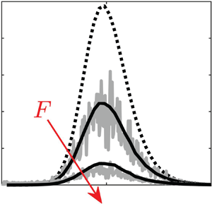
Figure 1. (a) Weakly and fully nonlinear stochastic gains (defined respectively in (3.7) and (3.8)) for the toy model (3.9),  $Re=160$. Inset: same for $Re=20$ (continuous blue line) and $Re=1280$ (dash-dotted red line), but in log–log scale and with the $x$-axis rescaled by the linear gain. (b) For the case $Re=160$, associated ensemble-averaged Fourier spectra of the response $\hat {\boldsymbol {u}}$ (where $\epsilon _o\hat {\boldsymbol {u}}_1 = \epsilon _o\hat {B}\boldsymbol {\hat {q}}$ in the WNNs approach and $\hat {\boldsymbol {u}}_p$ in the DNS), normalised such that $G$ is twice the area under the curve. Insets: single realisations of $\epsilon _o^2||\boldsymbol {u}_p(t)||^2/F^2$ as a function of time in the statistically steady regime (red solid line), and ensemble average in the linear regime (black dashed line).
3.2. Bilinear system and application to the backward-facing step flow
The weakly nonlinear evolution of the stochastic gain is now sought for the incompressible NSE. The nonlinear term  $C(\boldsymbol {U},\boldsymbol {U})$, where $C(\boldsymbol {a},\boldsymbol {b}) \doteq ( (\boldsymbol {b}\boldsymbol {\,\cdot \,}\boldsymbol {\nabla }) \boldsymbol {a} + (\boldsymbol {a}\boldsymbol {\,\cdot \,}\boldsymbol {\nabla }) \boldsymbol {b})/2$, is bilinear. Therefore, we expect essential nonlinear interactions to arise at third order in the expansion parameter, which we want to account for in the amplitude equation. Although it is certainly possible to correct (3.5) at order $O( {\epsilon_o^3} )$ after introducing a slower time scale $\tau _2$, it is simpler to rescale the forcing and the linear term such that they appear directly at the third order. In this manner, we avoid a response at second order, which would interact at the next order and obscure the amplitude equation unnecessarily.
We propose the rescaled multiple-scale expansion
 \begin{align} \boldsymbol{U}(t,\tau_1,\tau_2) = \boldsymbol{U}_e + \sqrt{\epsilon_o}\boldsymbol{u}_1(t,\tau_1,\tau_2) + \epsilon_o \boldsymbol{u}_2(t,\tau_1,\tau_2) + \sqrt{\epsilon_o}^3 \boldsymbol{u}_3(t,\tau_1,\tau_2) + O( \epsilon_o^2 ), \end{align}
where  $\tau _1 = \sqrt {\epsilon _o}t$ and $\tau _2 = \epsilon _o t$. The flow is weakly forced by $\boldsymbol {F}=\phi \sqrt {\epsilon _o}^3\boldsymbol {f}_o\xi (t)$ (a second advantage of the rescaling is that the forcing amplitude $F=\phi \sqrt {\epsilon _o}^3$ is larger than that previously defined by a factor $1/\sqrt {\epsilon _o}$). Following the method outlined in the previous section, we introduce (3.10) in the NSE, take the Fourier component at $\omega$ and perturb the inverse resolvent according to (2.9). The solution at $O( \sqrt {\epsilon _o} )$ is again $\hat {\boldsymbol {u}}_1(\tau _1,\tau _2;\omega ) = \hat {B}(\tau _1,\tau _2;\omega )\boldsymbol {\hat {q}}(\omega )$. At order $O( \epsilon _o )$ we obtain
 \begin{equation} \varPhi \hat{\boldsymbol{u}}_2 ={-}\boldsymbol{\hat{q}} \partial_{\tau_1}\hat{B} + \boldsymbol{\hat{g}}_2[\hat{B}], \end{equation}
with  $\boldsymbol {\hat {g}}_2[\hat {B}] = - \mathcal {F} [ C(\mathcal {F}^{-1} [ \hat {B}\boldsymbol {\hat {q}} ],\mathcal {F}^{-1} [ \hat {B}\boldsymbol {\hat {q}} ]) ]$. Imposing the Fredholm alternative such that the right-hand side ( $\doteq \boldsymbol {\hat {f}}_2$) of (3.11) is orthogonal to $\hat {\boldsymbol {a}}$ yields $\{ \hat {\boldsymbol {a}}, \boldsymbol {\hat {q}} \} \partial _{\tau _1}\hat {B}= \{ \hat {\boldsymbol {a}}, \boldsymbol {\hat {g}}_2[\hat {B}] \}=\hat {g}_2[\hat {B}]$. The field $\boldsymbol {\hat {u}}^{\perp }_2 \doteq R\boldsymbol {\hat {f}}_2$ is such that $\{ \boldsymbol {\hat {u}}^{\perp }_2, \boldsymbol {\hat {q}} \} = \{ \,\boldsymbol {\hat {f}}_2, \hat {\boldsymbol {a}} \} = 0$; thus $\varPhi \boldsymbol {\hat {u}}^{\perp }_2 = R^{-1}\boldsymbol {\hat {u}}^{\perp }_2$ and $\boldsymbol {\hat {u}}^{\perp }_2$ constitutes the particular solution of (3.11). The general solution can be written as $\hat {\boldsymbol {u}}_2 = \boldsymbol {\hat {u}}^{\perp }_2 + \hat {B}_2\boldsymbol {\hat {q}}$, with an arbitrary component $\hat {B}_2\boldsymbol {\hat {q}}$ on the kernel. We set $\hat {B}_2=0$ in the following, such that the component on $\boldsymbol {\hat {q}}$ of the overall response is fully embedded in $\hat {B}$, which can be corrected at higher order thanks to its dependence on slower time scales. Consequently,
 \begin{equation} \hat{\boldsymbol{u}}_{2}[\hat{B}] = \boldsymbol{\hat{u}}^{{\perp}}_{2}[\hat{B}] = R(\boldsymbol{\hat{g}}_2[\hat{B}] - \{ \hat{\boldsymbol{a}}, \boldsymbol{\hat{q}} \} ^{{-}1} \hat{g}_2[\hat{B}]\boldsymbol{\hat{q}} ). \end{equation}
 Collecting terms at  $O( \sqrt {\epsilon _o}^3 )$, injecting the expressions for $\hat {\boldsymbol {u}}_1$ and $\hat {\boldsymbol {u}}_2$ and using the Fredholm alternative leads to an expression for $\partial _{\tau _2}\hat {B}$,
 \begin{equation} \{ \hat{\boldsymbol{a}}, \boldsymbol{\hat{q}} \} \partial_{\tau_2}\hat{B} = \{ \hat{\boldsymbol{a}}, \boldsymbol{f}_o \}(\phi\hat{\xi}-\hat{B}) - \{ \hat{\boldsymbol{a}}, \partial_{\tau_1}\hat{\boldsymbol{u}}_2[\hat{B}] \} + \hat{g}_3[\hat{B}], \end{equation}
with the functional  $\hat {g}_3[\hat {B}] = - \{ \hat {\boldsymbol {a}}, \mathcal {F} [ 2C(\mathcal {F}^{-1} [ \hat {B}\boldsymbol {\hat {q}} ],\mathcal {F}^{-1} [ \hat {\boldsymbol {u}}_2[\hat {B}] ]) ] \}$. The total slow temporal evolution of $\hat {B}$ for a given frequency is found by combining partial derivatives with respect to the slow time scales (Orchini, Rigas & Juniper Reference Orchini, Rigas and Juniper2016) as $\mathrm {d}_{\tau _1}\hat {B} = \partial _{\tau _1}\hat {B} + (\partial _{\tau _1}/\partial _{\tau _2})\partial _{\tau _2}\hat {B} = \partial _{\tau _1}\hat {B} + \sqrt {\epsilon _o}\partial _{\tau _2}\hat {B}$. Eventually, it leads to leads to an ordinary differential equation for $\hat {B}$ (remember that $\boldsymbol {f}_h = \boldsymbol {f}_o$):
 \begin{equation} \{ \hat{\boldsymbol{a}}, \boldsymbol{\hat{q}} \} \mathrm{d}_{\tau_1} \hat{B} = \hat{g}_2[\hat{B}]+\sqrt{\epsilon_o}[ \{ \hat{\boldsymbol{a}}, \boldsymbol{f}_o \}(\phi\hat{\xi}-\hat{B}) +\hat{g}_3[\hat{B}] - \partial_{\tau_1} \{ \hat{\boldsymbol{a}}, \hat{\boldsymbol{u}}_2[\hat{B}] \} ]. \end{equation}
 An equilibrium solution  $\hat {B}(\omega )$ of (3.14) is sought for given choices of $\phi$ and phase distribution for $\hat {\xi }$. It is associated with the statistically steady stochastic gain (3.7). In the linear regime, $\phi \rightarrow 0$ and $\hat {B} \rightarrow \phi \xi$, so the gain reduces to $G=1/\epsilon _o^2$ as expected. All the nonlinear terms such as $\hat {g}_{2}[\hat {B}]$, $\hat {g}_{3}[\hat {B}]$ and $\partial _{\tau _1} \{ \hat {\boldsymbol {a}}, \hat {\boldsymbol {u}}_2[\hat {B}] \}$ are convolution integrals accounting for the nonlinear interactions between the Fourier modes. They can be discretised in the frequency domain as quadratic or cubic products of the Fourier components of $\hat {B}(\omega )$. Detailed expressions are given in the supplementary material § 2, together with an algorithm to solve for the equilibrium solution.
We now consider the weakly nonlinear evolution of the stochastic gain in the two-dimensional BFS flow at  $Re=500$. This flow clearly illustrates streamwise non-normality, as evidenced, for example, in Blackburn et al. (Reference Blackburn, Barkley and Sherwin2008). A Poiseuille profile of unit centreline velocity is imposed at the inlet. The nonlinear and linearised NSE are solved with the finite element method (see details in the supplementary material § 3). Figure 2(a) shows the optimal stochastic forcing $\boldsymbol {f}_o$, which is remarkably similar to the harmonic forcing structure at the optimal frequency $\omega =0.47$ determined via a resolvent analysis (Mantic-Lugo & Gallaire Reference Mantic-Lugo and Gallaire2016); the harmonic gain being maximal at $\omega =0.47$, the associated forcing structure is naturally favoured when maximising the stochastic gain. Figure 2(b) shows a DNS snapshot of the flow response to $F\xi (t)\boldsymbol {f}_o$ for $F=0.00025$.
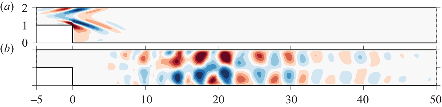
Figure 2. (a) Streamwise component of the optimal stochastic forcing  $\boldsymbol {f}_o$ in the BFS flow, $Re=500$. (b) DNS snapshot of the associated streamwise velocity response (around the base flow) for $F=0.00025$.
The results of the WNNs model are reported in figure 3, where the amplitude equation (3.14) for  $\mathrm {d}_{\tau _1}\hat {B}=0$ was uniformly discretised with $N$ frequencies $\omega \in [0,\omega _c]$ with $\omega _c={\rm \pi}$, and the results were ensemble-averaged over $500$ realisations of the white noise. Predictions from the DNS are also shown, resulting from simulations of duration $T=2049$ after the transients fade away, sampled at $\Delta t = {\rm \pi}/\omega _c = 1$ and ensemble-averaged over $10$ realisations of the white noise (this lower number of realisations is the consequence of each one being numerically costly). Unlike the toy model of § 3.1, the amplitude equation built from a forcing introduced at second order and stopped at second order did not capture significant nonlinear effects (not shown). Introducing instead the forcing at third order, as described above, the comparison with DNS data is conclusive: the stochastic gains experience a monotonic decay with increasing $F$, also associated with a decreasing standard deviation for the DNS data.

Figure 3. Same as figure 1 for the BFS flow,  $Re=500$. Error bars around DNS points show plus or minus one standard deviation.
We now emphasise that the fully nonlinear stochastic gain in (3.8) considers perturbation around the temporal mean flow, and not around the base flow  $\boldsymbol {U}_e$. This distinction was unimportant in the previous application case since the nonlinearity did not generate a temporal mean. The creation of non-zero temporal mean ( $\overline {\boldsymbol {U}(t)}\neq 0$) is associated with a diverging behaviour of the Fourier component at $\omega =0$, as the normalisation in (2.4a,b) directly implies $\hat {\boldsymbol {U}}(0)=\overline {\boldsymbol {U}(t)} \sqrt {T} \rightarrow \infty$. Since this divergence is unlikely to be captured by $\hat {B}(0)$, we omitted its contribution in the gain calculation, but noted that this did not change the gain. However, the WNNs model certainly takes into account the effects of temporal mean flow corrections on $\hat {\boldsymbol {u}}_1(\omega )$, as such steady corrections are created at the next order and embedded in $\boldsymbol {u}_2(t)$.
For small  $F$ close to the linear regime, DNS and WNNs show some discrepancies (figure 3a) that are believed to be due to an imperfect convergence of the DNS data, because of the large standard deviation at small $F$ and the limited number of realisations. The limit of large $F$ is also associated with a slight departure of the (well-converged) DNS data from the WNNs predictions, although it is believed this time to be due solely to increasingly strong nonlinearities. In figure 3(b), the Fourier spectra reveal that increasing $F$ conserves the most amplified frequency, which may be due to the fact that the forcing structure is fixed to $\boldsymbol {f}_o$, extremely similar to the optimal harmonic forcing for $\omega =0.47$. In the inset, from the temporal evolution of the signal $\propto ||\boldsymbol {u}(t)||^2$ we recover that, for this particular flow, nonlinearities not only saturate the average level of energy of the response, but also significantly reduce the amplitude of the oscillations (i.e. the standard deviation).
Finally, note that the asymptotic expansions (3.1) and (3.10) have been scaled differently in order for the linear ( $\propto \hat {B}$) and forcing ( $\propto \phi \hat {\xi }$) terms to appear at the last considered order. This raises the question of how to know a priori, and for a given nonlinearity, the minimal order that should be considered. Although a ‘trial and error’ process is always arguably acceptable, we postulate that it is the earliest order where the nonlinear term generates a component oscillating at $\omega _o$, in the limit where the linear response $\boldsymbol {\hat {q}}$ is monochromatic and oscillating at $\omega _o$. Indeed, if we impose the solvability condition solely at the order(s) before, $\hat {B}$ will conserve its linear value, for the nonlinear term will naturally yield a null scalar product with the adjoint for all frequencies (both fields being non-zero at different frequencies). This scenario, which we want to avoid, does not occur in the opposite limit where the frequency spectrum of $\boldsymbol {\hat {q}}$ is flat. Of course, the linear optimal response has generally no reason to be monochromatic, but might still show a maximum in energy at selective frequencies, as was the case in figures 1(b) and 3(b). If we express $\boldsymbol {u}_1=\hat {B}\boldsymbol {\hat {q}} {\rm e}^{{\rm i}\omega _o t}+{\rm c.c.}$, the nonlinearity of the toy system at second order (i.e. $||\boldsymbol {u}_1||\boldsymbol{\mathsf{M}}\boldsymbol {u}_1$) already generates terms oscillating at $\omega _o$; therefore it was sufficient to consider only up to this second order to see an improvement over the linear prediction. For the NSE, however, one needs to go to the third order to recover terms in $\omega _o$ (specifically $\hat {B}|\hat {B}|^2{\rm e}^{{\rm i} \omega _o t}$, as well known for classical weakly nonlinear equations for an eigenmode amplitude).
4. Conclusions
By generalising the method proposed in Ducimetière et al. (Reference Ducimetière, Boujo and Gallaire2022), we have derived an amplitude equation describing the weakly nonlinear, statistically steady response to stochastic forcing in arbitrarily stable yet non-normal systems. The amplitude depends solely on the frequency, and is therefore independent of the number of spatial degrees of freedom of the discretised system. This may save a significant amount of computational resources compared to fully nonlinear simulations, where long simulated times and/or many realisations are needed to ensure statistical convergence, which becomes rapidly impracticable for large systems like fluid flows. The amplitude equation has been successfully compared to fully nonlinear numerical simulations, and predicts well the variation of both the stochastic gain and the Fourier spectrum with the forcing amplitude.
Future research may include applying the method to realistic flows (e.g. atmospheric flows subject to weak forcing, such as zonal jets in barotropic flows (Bouchet, Nardini & Tangarife Reference Bouchet, Nardini and Tangarife2013)), and developing extensions towards systems with multiple attractors and noise-induced transition.
Supplementary material
Supplementary material is available at https://doi.org/10.1017/jfm.2022.902.
Acknowledgements
The authors would like to thank the anonymous referees for constructive questions and comments on the manuscript.
Funding
We acknowledge the Swiss National Science Foundation under grant 200341.
Declaration of interests
The authors report no conflict of interest.
Appendix A. Toy system: nonlinear upshift of the most amplified frequency
In figure 1(b), the peak of the linear response in  $\omega =0$ is due to the presence of both eigenvalues on the imaginary axis (although their location alone is insufficient to deduce the stochastic gain, due to the non-normality of the operator). We explain the shift of the peak to higher frequencies with increasing nonlinearities as follows.
The equilibrium solution ( $\mathrm {d}_{\tau _1}\hat {B}=0$) of the amplitude equation (3.5) reads
 \begin{equation} \hat{B} = \epsilon_o ||\boldsymbol{\hat{q}}||^{{-}2} \hat{g}_2[\hat{B}] + \phi\hat{\xi} , \end{equation}
where we used that  $\{ \hat {\boldsymbol {a}}, \boldsymbol {f}_o \} = \{ \boldsymbol {\hat {q}}, \boldsymbol {\hat {q}} \}/\epsilon _o = ||\boldsymbol {\hat {q}}||^2/\epsilon _o$. We plot in figure 4 the ensemble average of the absolute values of: (1) the solution, $\langle |\hat {B}| \rangle$; (2) the nonlinear term, $\epsilon _o ||\boldsymbol {\hat {q}}||^{-2} \langle |\hat {g}_2[\hat {B}]| \rangle$; (3) the same nonlinear term but replacing $\hat {B}$ by its solution in the linear regime $\phi \hat {\xi }$, i.e. $\epsilon _o||\boldsymbol {\hat {q}}||^{-2} \langle |\hat {g}_2[\phi \hat {\xi }]| \rangle$; and (4) the linear stochastic forcing term, $\langle |\phi \hat {\xi }| \rangle = \langle \phi \rangle = \phi$. In the linear regime for $F=10^{-16}$ ( $\phi \rightarrow 0$) in figure 4(a), $\hat {B}=\phi \hat {\xi }$ is the solution, for the nonlinear term $\hat {g}_2$ is virtually zero. However, when we increase the forcing up to $F=2 \times 10^{-7}$ in figure 4(b), the nonlinear interaction of the linear (optimal) response $\phi \hat {\xi } \boldsymbol {\hat {q}}$ with itself is no longer negligible and creates a strong response peaked around $\omega = 0$, which projects back on the optimal response (see dash-dotted blue line in figure 4b). Thereby, $\hat {B}=\phi \hat {\xi }$ cannot be the solution any more, and $\hat {B}$ must adapt around $\omega =0$ so as to enforce the solvability condition. In more physical terms, $\hat {B}$ must adapt around $\omega =0$ such that the nonlinear interaction of $\hat {B} \boldsymbol {\hat {q}}$ with itself is less amplified around $\omega =0$ than that of $\phi \hat {\xi } \boldsymbol {\hat {q}}$, thus preserving the asymptotic hierarchy.

Figure 4. Ensemble averages: (a)  $F=10^{-16}$. (b) $F=2\times 10^{-7}$.
This is indeed what we observe in figure 4(b), where the red curve (with the bullet markers) is significantly less amplified than the dashed blue one. Whether this new  $\hat {B}$ must have a larger or smaller amplitude than its linear value $\phi$ is given by the phase difference, which we call $\gamma$, between the nonlinear and the forcing terms in (A1). It is easy to show that $|\hat {B}| \leqslant \phi$ if and only if
 \begin{equation} {-}2\phi\cos(\gamma) \geqslant \epsilon_o ||\boldsymbol{\hat{q}}||^{{-}2}|\hat{g}_2[\hat{B}]|. \end{equation}
For this reason we show  $-2\phi \langle \cos (\gamma ) \rangle$ in figure 4(b) (see the magenta dotted line). In the range $0 \leqslant \omega \leqslant 0.012$, $\langle \cos (\gamma ) \rangle$ decreases monotonically from $-1$ at $\omega =0$ (the forcing and the nonlinear terms are in antiphase) to $-0.2$ at $\omega =0.012$. In addition, the magenta dotted line is above the red one, thus $\langle |\hat {B}| \rangle \leqslant \phi$ and the nonlinearities are saturating in the sense that the weakly nonlinear response is of lower amplitude than the linear one. On the contrary, for $\omega \geqslant 0.012$ the phase difference between the forcing and the nonlinear terms is such that $\langle |\hat {B}| \rangle \geqslant \phi$ and the nonlinearities are desaturating. Therefore, the maximum of $||\hat {B}\boldsymbol {\hat {q}}||$ is now increased to $\omega =0.005$. This tendency is conserved for all the considered $F$.
$F$.


 Open access