2.1. Problem description

The flow configuration studied in this article is shown in figure 1, and is similar to the set-up used by Zhang et al. (Reference Zhang, Shen and Yue1999). We consider a vortex ring with initial circulation $\varGamma _0$, ring radius $R_0$ and core radius $a$, positioned at an initial depth $H$ beneath a free surface. The vortex ring is inclined, and approaches the free surface at an angle $\alpha$. While the main focus of this article is on free-surface flows, we also consider the interaction between a vortex ring and a fluid–fluid interface. For the two-fluid case, we must consider the fluid domains below (fluid 1) and above (fluid 2) the interface, while we consider only the lower fluid (fluid 1) in the free-surface case. The free surface is an approximation for the fluid–fluid interface, in the limit that density and viscosity of the upper fluid approach zero.

Figure 1. Flow configuration considered in this study. A vortex ring of circulation $\varGamma _0$, radius $R_0$ and core radius $a$ is positioned at depth $H$ beneath the interface (or free surface), and approaches the interface at angle $\alpha$. The computational domain is a box with side lengths $L_x$, $L_y$, and $L_{z,1}$ (in fluid 1) and $L_{z,2}$ (in fluid 2). For free-surface flows, the upper fluid is ignored, and the interface is replaced with the free-surface boundary.

Assuming incompressible flow, the continuity and momentum equations in each fluid are written as

(2.1)\begin{gather} \boldsymbol{\nabla} \boldsymbol{\cdot} \boldsymbol{u}_i = 0, \end{gather}

(2.2)\begin{gather}\frac{\partial {\boldsymbol{u}_i}}{\partial {t}} + \boldsymbol{u}_i \boldsymbol{\cdot} \boldsymbol{\nabla} \boldsymbol{u}_i ={-}\frac{1}{\rho_i}\,\boldsymbol{\nabla} p_i + \boldsymbol{g} + \nu_i\, {\nabla}^{2} \boldsymbol{u}_i, \end{gather}

where subscript $i = 1,2$ indicates quantities defined in fluids 1 and 2, respectively. Density is denoted by $\rho$, and the dynamic and kinematic viscosities are denoted $\mu$ and $\nu$, respectively. Finally, $\boldsymbol {g}$ is the acceleration due to gravity.

Following Zhang et al. (Reference Zhang, Shen and Yue1999), flow parameters are non-dimensionalised by the initial circulation ($\varGamma _0$) and radius ($R_0$) of the vortex ring, and the density of the lower fluid ($\rho _1$). The following dimensionless parameters are then used to characterise this flow: the Reynolds number $Re = \varGamma _0/\nu _1$, the Froude number $Fr = \varGamma _0/g^{1/2}R_0^{3/2}$, the Weber number $We = R_0 \sigma /(\rho _1 \varGamma _0^{2})$, the initial depth to radius ratio $H/R_0$, and the initial vortex core to ring diameter ratio, $a/R_0$. The effects of surface tension, $\sigma$, are not considered in this article, thus the Weber number is set to $We = 0$. For two-fluid flows, the ratios of density ($\rho _1/\rho _2$) and dynamic viscosity ($\mu _1/\mu _2$) across the interface must also be considered.

We generate the initial velocity field using the approach outlined in Zhang et al. (Reference Zhang, Shen and Yue1999). First, we assume a Gaussian profile for the initial vorticity distribution in the vortex core,

(2.3)\begin{equation} \omega_{{axial}} = \frac{\varGamma_0}{{\rm \pi} a^{2}} \exp{\left(\frac{r^{2}}{a^{2}}\right)},\end{equation}

where $\omega _{{axial}}$ is the vorticity component aligned with the vortex core axis, and $r$ is the distance from the vortex axis. Then a streamfunction is obtained by solving the Poisson equation

(2.4)\begin{equation} {\nabla}^{2} \boldsymbol{\varPsi} ={-}\boldsymbol{\omega}\end{equation}

with boundary conditions $\varPsi _x = \varPsi _y = \partial \varPsi _z /\partial z = 0$ on the free surface, and $\boldsymbol {\varPsi } = 0$ for all remaining boundaries. Then the initial velocity field is obtained from the streamfunction:

(2.5)\begin{equation} \boldsymbol{u} = \boldsymbol{\nabla} \times \boldsymbol{\varPsi}. \end{equation}

Note that the Gaussian profile is not a steady-state solution, and the ring undergoes an adjustment to a more stable profile at the beginning of the simulation (Zhang et al. Reference Zhang, Shen and Yue1999).

2.2. Interfacial boundary conditions

The following boundary conditions are used for a fluid–fluid interface. First is the continuity of velocity,

(2.6)\begin{equation} \boldsymbol{u}_1 = \boldsymbol{u}_2, \end{equation}

which is due to both the no-slip and no-penetration conditions. The remaining boundary conditions are due to the balance of tangential and normal stresses on the interface (Tuković & Jasak Reference Tuković and Jasak2012):

(2.7)\begin{gather} \mu_2(\hat{\boldsymbol{s}} \boldsymbol{\cdot} \boldsymbol{\nabla}\boldsymbol{u}_\parallel)_2 - \mu_1(\hat{\boldsymbol{s}} \boldsymbol{\cdot} \boldsymbol{\nabla} \boldsymbol{u}_\parallel)_1 ={-}\boldsymbol{\nabla}_\parallel \sigma - (\mu_2-\mu_1)(\boldsymbol{\nabla}_\parallel (\boldsymbol{u} \boldsymbol{\cdot} \hat{\boldsymbol{s}})), \end{gather}

(2.8)\begin{gather}p_2 - p_1 = \sigma \kappa - 2 (\mu_2 - \mu_1) \boldsymbol{\nabla}_\parallel \boldsymbol{\cdot} \boldsymbol{u}. \end{gather}

In (2.7) and (2.8), $\hat {\boldsymbol {s}}$ is the unit normal vector to the surface, $\boldsymbol {\nabla }_\parallel$ is the surface gradient operator, and $\kappa = -\boldsymbol {\nabla }_\parallel \boldsymbol {\cdot } \hat {\boldsymbol {s}}$ is the mean curvature of the interface. Also, $\boldsymbol {u}_\parallel = \boldsymbol {u} - (\boldsymbol {u} \boldsymbol {\cdot } \hat {\boldsymbol {s}})\hat {\boldsymbol {s}}$ is the surface-parallel velocity.

For a free surface, the upper fluid exerts no stresses on the lower fluid, apart from a constant pressure (Lundgren & Koumoutsakos Reference Lundgren and Koumoutsakos1999). Then the tangential and normal shear-stress balances in (2.7) and (2.8) reduce to the boundary conditions

(2.9)\begin{gather} \mu_1(\hat{\boldsymbol{s}} \boldsymbol{\cdot} \boldsymbol{\nabla} \boldsymbol{u}_\parallel)_1 -\boldsymbol{\nabla}_\parallel \sigma + \mu_1(\boldsymbol{\nabla}_\parallel (\boldsymbol{u} \boldsymbol{\cdot} \hat{\boldsymbol{s}})) = 0, \end{gather}

(2.10)\begin{gather}p_2 - p_1 = \sigma \kappa + 2 \mu_1 \boldsymbol{\nabla}_\parallel \boldsymbol{\cdot} \boldsymbol{u}. \end{gather}

2.3. The interTrackFoam solver

A key concern for the numerical simulations performed in this study is accurate determination of the boundary vorticity flux, which is given by the vorticity gradients at the free surface (see § 4.1). To this end, interface tracking schemes are preferred, as they allow vorticity gradients to be computed using grid points that lie on the interface. The primary numerical method used in this study is a moving-mesh interface tracking scheme, interTrackFoam (Tuković & Jasak Reference Tuković and Jasak2012), from the open-source software package, foam-extend 4.1 (a fork of the OpenFOAM software). The interTrackFoam solver uses an arbitrary Lagrangian–Eulerian (ALE) scheme to track motion of the interface, and can be applied to both single-fluid (free surface) or two-fluid (interfacial) flows.

The interTrackFoam solver is described in Tuković & Jasak (Reference Tuković and Jasak2012), and was validated against several test cases in that article. It has also been used (sometimes in a modified form) to study the motion of free-rising bubbles (Pesci et al. Reference Pesci, Weiner, Marschall and Bothe2018; Charin et al. Reference Charin, Lage, Silva, Tuković and Jasak2019), Taylor bubbles (Marschall et al. Reference Marschall, Boden, Lehrenfeld, Falconi, Hampel, Reusken, Wörner and Bothe2014) and transient capillary rise (Gründing et al. Reference Gründing, Smuda, Antritter, Fricke, Rettenmaier, Kummer, Stephan, Marschall and Bothe2020). It has been validated against other numerical methods (Gründing et al. Reference Gründing, Smuda, Antritter, Fricke, Rettenmaier, Kummer, Stephan, Marschall and Bothe2020; Marschall et al. Reference Marschall, Boden, Lehrenfeld, Falconi, Hampel, Reusken, Wörner and Bothe2014), as well as experimental measurements (Marschall et al. Reference Marschall, Boden, Lehrenfeld, Falconi, Hampel, Reusken, Wörner and Bothe2014), and good agreement has been obtained.

The interTrackFoam solver uses a finite volume-method, where the incompressible continuity and momentum equations are integrated across a set of control volumes,

(2.11)\begin{gather} \oint_{\partial V} \rho_{{i}} \hat{\boldsymbol{n}} \boldsymbol{\cdot} \boldsymbol{u}_{{i}} \,\mathrm{d}S = 0, \end{gather}

(2.12)\begin{gather}\frac{\mathrm{d} {}}{\mathrm{d} t}\int_V \rho_{{i}} \boldsymbol{u}_{{i}}\,\mathrm{d} V + \oint_{\partial V} \hat{\boldsymbol{n}} \boldsymbol{\cdot} \rho_{{i}} (\boldsymbol{u}_{{i}} - \boldsymbol{v}) \boldsymbol{u}_{{i}} \,\mathrm{d} S = \oint_{\partial V} \hat{\boldsymbol{n}} \boldsymbol{\cdot} (\mu_{{i}} \boldsymbol{\nabla} \boldsymbol{ u}_{{i}}) \,\mathrm{d} S - \int_V \boldsymbol{\nabla} {{\hat{p}_{{i}}}} \,\mathrm{d} V, \end{gather}

where $V$ is the control volume, and $\hat {\boldsymbol {n}}$ is the outward-oriented unit vector to the control-volume boundary. Also, $\boldsymbol {u}$ is the fluid velocity, $\nu$ is the dynamic viscosity, and $\hat {p}_{{i}}$ is the static pressure minus the hydrostatic pressure ($\hat {p}_{{i}} = p_{{i}} - \rho _{{i}} g z$). Finally, $\boldsymbol {v}$ is the velocity of the control-volume boundary, which may be different from the fluid velocity. Once again, subscript $i = 1,2$ indicates quantities defined in the lower and upper fluids, respectively.

The advantage of this scheme is that the computational mesh is allowed to move, with velocity $\boldsymbol {v}$, so that grid points track the interface as it moves. This requires that on the free surface, the surface-normal velocity of the mesh matches the fluid velocity:

(2.13)\begin{equation} \boldsymbol{v} \boldsymbol{\cdot} \hat{\boldsymbol{s}} = \boldsymbol{u}_1 \boldsymbol{\cdot} \hat{\boldsymbol{s}} = \boldsymbol{u}_2 \boldsymbol{\cdot} \hat{\boldsymbol{s}}.\end{equation}

To ensure that the internal mesh remains smooth, the velocity of internal grid points is obtained from the velocity on the boundary using a mesh-motion solver (Jasak & Tukovic Reference Jasak and Tukovic2006). Since the numerical mesh moves with the interface, the boundary conditions (2.6)–(2.10) can be applied directly to the interface or free surface. Details on how these boundary conditions are implemented in the interTrackFoam solver can be found in Tuković & Jasak (Reference Tuković and Jasak2012).

In the interTrackFoam solver, (2.11) and (2.12) are discretised using the finite-volume method. Spatial derivatives are converted to boundary fluxes on control-volume faces using Gauss’ theorem, and linear interpolation was used to construct the fluxes on cell faces. Time is divided into discrete time steps, and the temporal derivative is discretised using a second-order backwards time scheme,

(2.14)\begin{equation} \frac{\partial {}}{\partial {t}}(\phi^{(n)}) = \frac{1}{\Delta t}\left(\frac{3}{2}\,\phi^{(n)} - 2 \phi^{(n-1)} + \frac{1}{2}\,\phi^{(n-2)} \right), \end{equation}

where $n$ is the current time step. Finally, the discretised equations are solved using an iterative method, based on the PISO algorithm (Issa Reference Issa1986). For further details on how this method is implemented, refer to Tuković & Jasak (Reference Tuković and Jasak2012).

2.4. Volume-of-fluid method

To validate the results of the interTrackFoam solver, additional simulations are performed using the volume-of-fluid (VOF) method (Hirt & Nichols Reference Hirt and Nichols1981). Two different implementations of the VOF method were used: the interFoam solver from foam-extend 4.1, and the VOF method implemented in the commercial software package ANSYS FLUENT.

Instead of tracking the interface directly, the VOF method introduces a volume fraction $F$ that indicates the fraction of each fluid contained in a given control volume. For two-fluid flows, $F=1$ for cells that contain only the lower fluid (fluid 1), while $F=0$ for cells containing only the upper fluid (fluid 2). For cells that contain the interface between two fluids, the volume fraction lies in the interval $0 < F < 1$. The interface is therefore captured indirectly, via the evolution of the volume fraction field.

For incompressible flows, with no mass transfer between phases, the volume fraction satisfies the conservation law (Hirt & Nichols Reference Hirt and Nichols1981)

(2.15)\begin{equation} \frac{\partial {F}}{\partial {t}} + \boldsymbol{\nabla} \boldsymbol{\cdot} (\boldsymbol{u} F) = 0.\end{equation}

However, care must be taken to ensure that the interface remains sharp when solving this equation (Hirt & Nichols Reference Hirt and Nichols1981). In the interFoam solver, this is achieved by modifying the advective fluxes near the interface (Deshpande, Anumolu & Trujillo Reference Deshpande, Anumolu and Trujillo2012), by incorporating an interface compression term. In ANSYS FLUENT, the geometric reconstruction scheme was used (ANSYS 2019) to maintain a sharp interface.

In the VOF method, a single set of momentum equations is solved for both fluids, across the entire computational domain (Deshpande et al. Reference Deshpande, Anumolu and Trujillo2012):

(2.16)\begin{equation} \frac{\partial {}}{\partial {t}}{\rho \boldsymbol{u}} + \boldsymbol{\nabla} \boldsymbol{\cdot} (\rho \boldsymbol{u}\boldsymbol{u}) ={-}\boldsymbol{\nabla} p + \left[\boldsymbol{\nabla} \boldsymbol{\cdot} (\mu\,\boldsymbol{\nabla} \boldsymbol{u}) + \boldsymbol{\nabla} \boldsymbol{u} \boldsymbol{\cdot} \boldsymbol{\nabla} \mu \right] + \rho \boldsymbol{g}.\end{equation}

In this equation, fluid properties, such as density and viscosity, are taken to be average values based on the volume fraction:

(2.17a)\begin{gather} \rho = F \rho_1 + (1-F) \rho_2, \end{gather}

(2.17b)\begin{gather}\mu = F \mu_1 + (1-F) \mu_2. \end{gather}

Equations (2.15) and (2.16) are discretised using the finite-volume approach. For details of the numerical implementation, refer to Deshpande et al. (Reference Deshpande, Anumolu and Trujillo2012) for the implementation in interFoam, and to ANSYS (2019) for the implementation in ANSYS FLUENT.

We remark that typically, vorticity and vorticity gradients exhibit a discontinuity across the interface (Terrington et al. Reference Terrington, Hourigan and Thompson2022). However, under the VOF method, this discontinuity is spread over a region near the interface where $0< F<1$, which leads to difficulty in determining the boundary vorticity flux at the interface. Therefore, the interface tracking interTrackFoam solver is preferred for this study, and the VOF method is used mainly to validate the results of the interTrackFoam solver.

2.5. Mesh generation

The computational domain considered in this study is illustrated in figure 1. The computational domain is a rectangular box with side lengths $L_x$ and $L_y$ in the streamwise ($x$) and spanwise ($y$) directions, respectively. The interface is initially situated at elevation $z=0$, and the computational domain extends to depth $L_{z,1}$ below the interface. For free-surface simulations, the upper boundary of the computational domain is located on the free surface, while for two-fluid simulations, the computational domain extends to elevation $L_{z,2}$ above the interface. Unless otherwise stated, the computational domain used in this study has side lengths $L_x/R_0 = 20$, $L_y/R_0 = 20$, $L_{z,1}/R_0 = 10$ and $L_{z,2}/R_0 = 5$.

When using the interTrackFoam solver, the interface (or free surface) forms part of the computational domain boundary, and the numerical mesh will deform with the surface. For two-fluid simulations, separate meshes are used for the upper and lower fluids, with the interface forming the boundary between these meshes. For free-surface flows, only a single mesh is used, with a boundary on the free surface. When the VOF method is used, a single stationary grid is used for the entire computational domain, and the interface is not part of the computational domain boundary.

The computational domain was meshed using a block-structured approach, as illustrated in figure 2. A fine grid was used in the region near the vortex ring, bounded by $-2\leqslant x\leqslant 2$, $-3\leqslant y \leqslant 3$ and $-3.5 \leqslant z \leqslant 0$, with a lower grid resolution used outside this region. Additionally, the cell size in the vertical ($z$) direction was reduced near the interface, to capture accurately vorticity gradients near the surface. For simulations run in foam-extend 4.1, meshes were generated using the blockMesh application, while for simulations run in ANSYS FLUENT, the mesh was generated using ICEM CFD.

Figure 2. An example of the meshing scheme used in this study, viewed from (a) the $x$–$z$ plane, and (b) the $y$–$z$ plane. Dark lines divide regions with different mesh grading. The locations of the representative cell sizes in table 1 are also shown. For clarity, the grid shown here is much coarser than those used for numerical simulations. For single-fluid simulations, the mesh in the upper fluid is removed, and the free surface ($z = 0$) is the upper boundary of the computational domain.

Table 1. Numerical grids used in the convergence study, where $N$ is the total number of cells, while $\Delta x$, $\Delta y$ and $\Delta z$ indicate the cell spacing in the fine-mesh region (figure 2). Spacing in the $z$ direction is provided at both $z = -3.5$ ($\Delta z_{(3.5)}$), and at the interface ($\Delta z_{(0)}$).

Simulations were performed in a Galilean reference frame, translating with a velocity approximately equal to the vortex ring velocity, to ensure that the vortex ring remained within the fine-mesh region. This was achieved by applying a constant velocity inlet to the upstream boundary (at $x = +L_x$), with inlet velocity $U_\infty /(\varGamma _0/R_0) = (-0.1,0,0)$. Outlet boundary conditions were applied to the downstream boundary (at $x = -L_x$), while the remaining boundaries, aside from the interface, were set to free-slip walls.

2.6. Validation study

A grid resolution study was performed using the meshes outlined in table 1, where mesh 1 has the coarsest resolution, and mesh 3 has the finest resolution. Simulations were run using interTrackFoam, for a single-fluid free-surface flow. Physical parameters were chosen to match Case 2 from Zhang et al. (Reference Zhang, Shen and Yue1999): $Re = 1570$, $Fr = 0.47$, $\alpha = 80^{\circ }$, $H/R_0 = 1.57$ and $a/R_0 = 0.35$.

In figure 3, we plot the maximum spanwise vorticity ($\omega _y$) in the symmetry plane ($y=0$), normalised by the initial peak vorticity ($\omega _0$), for each mesh resolution. The maximum vorticity in the symmetry plane is nearly identical between meshes 2 and 3, demonstrating that adequate resolution has been obtained in this region. The maximum vertical vorticity ($\omega _z$) in the free surface is also provided in figure 3. Noting convergence of the predictions between resolutions and that the differences in the maximum vorticity between meshes 2 and 3 are relatively small, the grid resolution is assumed satisfactory. The finest mesh (mesh 3) is used for all subsequent simulations in this study.

Figure 3. Grid resolution study, showing the maximum magnitude of spanwise vorticity ($\omega _y$) in the symmetry plane (solid lines), as well as the maximum vertical vorticity ($\omega _z$) in the free surface (dashed lines), for the meshes defined in table 1. The physical parameters match Case 2 from Zhang et al. (Reference Zhang, Shen and Yue1999): $Re = 1570$, $Fr = 0.47$, $\alpha = 80^{\circ }$, $H/R_0 = 1.57$ and $a/R_0 = 0.35$.

The grid resolution study was performed using identical physical parameters to Case 2 from Zhang et al. (Reference Zhang, Shen and Yue1999), in order to validate our results against their simulations. However, as shown in figure 4, the profiles of maximum vorticity magnitude, in both the symmetry plane and the free surface, are vastly different. In our simulations, the maximum vorticity in the symmetry plane increases to over 2.8 times the initial peak vorticity, as the vortex ring interacts with the free surface, while Zhang et al. (Reference Zhang, Shen and Yue1999) report a monotonic decrease in the vorticity magnitude. In both cases, the maximum value of vertical vorticity in the free surface is of a magnitude similar to the maximum vorticity in the symmetry plane, and is therefore much higher in our simulations ($\approx 2.5 \omega _0$), compared to Zhang et al. ($\approx 0.9 \omega _0$). The time scales over which reconnection occurs also appear to be different between our results; however, it is unclear if Zhang et al. use a physical or dimensionless flow time. In figure 5, we assume that Zhang et al. use a physical flow time, corresponding to the experimental parameters used by Gharib et al. (Reference Gharib, Weigand, Willert and Leipmann1994), and the time scale for vortex connection matches our solution.

Figure 4. Comparison between (a) our simulation, and (b) that of Zhang et al. (Reference Zhang, Shen and Yue1999), showing the maximum spanwise vorticity in the symmetry plane (solid lines), and the maximum vertical vorticity ($\omega _z$) in the free surface (dashed lines). The physical parameters are $Re = 1570$, $Fr = 0.47$, $\alpha = 80^{\circ }$, $H/R_0 = 1.57$ and $a/R_0 = 0.35$.

Figure 5. Comparison between the current numerical results (interTrackFoam), the numerical simulations of Zhang et al. (Reference Zhang, Shen and Yue1999), and the experimental measurements of Gharib et al. (Reference Gharib, Weigand, Willert and Leipmann1994), showing the maximum spanwise vorticity in the symmetry plane (solid lines), and vertical vorticity in the free surface (dashed lines). The physical parameters are $Re = 1150$, $Fr = 0.19$, $\alpha = 83^{\circ }$, $H/R_0 = 2$ and $a/R_0 = 0.3$. Results from the interTrackFoam solver when averaged over the interrogation window from the experimental particle image velocimetry (PIV) measurements are also presented.

Zhang et al. (Reference Zhang, Shen and Yue1999) validate their numerical method against the experimental measurements of Gharib et al. (Reference Gharib, Weigand, Willert and Leipmann1994). We performed an additional validation simulation using physical parameters matching the experimental conditions: $Re = 1150$, $Fr = 0.19$, $\alpha = 83^{\circ }$, $H/R_0 = 2$, and $a/R_0 = 0.3$, and the results are presented in figure 5. The Zhang et al. simulations are in reasonable agreement with the experimental measurements of Gharib et al., whereas our simulations are remarkably different. Once again, we find a sharp increase in the maximum spanwise vorticity during the vortex reconnection process, while Zhang et al. (Reference Zhang, Shen and Yue1999) and Gharib et al. (Reference Gharib, Weigand, Willert and Leipmann1994) report no increase in the maximum spanwise vorticity.

Since numerical simulations performed using the interTrackFoam solver disagree with existing numerical and experimental results, we performed simulations using the VOF method, for the same physical parameters. The VOF method requires two fluids, and the density and viscosity ratios were set to $\rho _1/\rho _2 = 1000$ and $\mu _1/\mu _2 = 100$, so the influence of the upper fluid is small. A comparison between the different numerical methods used (interTrackFoam, for both free-surface and two-fluid flows, and the VOF method, using both interFoam, and ANSYS FLUENT) is shown in figure 6, for physical parameters matching Case 2 from Zhang et al. (Reference Zhang, Shen and Yue1999). The maximum vorticities in the symmetry plane are nearly identical for each method, providing support for the interTrackFoam solver.

Figure 6. Comparison between the different numerical methods used in this study, showing maximum magnitude of spanwise vorticity in the symmetry plane, for physical parameters $Re = 1570$, $Fr = 0.47$, $\alpha = 80^{\circ }$, $H/R_0 = 1.57$ and $a/R_0 = 0.35$.

Moreover, the sharp rise in spanwise vorticity seen in our simulations is also observed in symmetrical vortex ring connections (Kida, Takaoka & Hussain Reference Kida, Takaoka and Hussain1991), which are equivalent to a perfectly flat (zero Froude number) free surface. To simulate a flat free surface, simulations were performed using the pimpleFoam solver in foam-extend 4.1, with the free surface replaced by a free-slip wall. In figure 7(a), we compare our results to the numerical simulations of Kida et al. (Reference Kida, Takaoka and Hussain1991) and Balakrishnan (Reference Balakrishnan2013), at $Re = 1153$, $\alpha = 90^{\circ }$, $a/R_0 = 0.4$ and $H/R_0 = 1.858$, in a periodic (in the $x$ and $y$ directions) box with side lengths $L_x/R_0 = 6.4$, $L_y/R_0 = 6.4$ and $L_z/R_0 = 4.5$. Results are in good agreement, and the slight disagreement can be attributed to the orientation of our periodic box (which differs from theirs by $45^{\circ }$). Importantly, we observe a sharp rise in the maximum spanwise vorticity in the initial stages of the connection process.

Figure 7. (a) Comparison between a flat shear-free surface (pimpleFoam) and the collision between two vortex rings (Kida et al. Reference Kida, Takaoka and Hussain1991; Balakrishnan Reference Balakrishnan2013), for physical parameters $Re = 1153$, $\alpha = 90^{\circ }$, $a/R_0 = 0.4$ and $H/R_0 = 1.858$. (b) Comparison between a flat shear-free surface (pimpleFoam) and a free surface (interTrackFoam), for $Re = 1570$, $\alpha = 80^{\circ }$, $H/R_0 = 1.57$ and $a/R_0 = 0.35$. Solid lines indicate the maximum spanwise vorticity ($\omega _y$) in the symmetry plane, while dashed lines indicate the maximum vertical vorticity ($\omega _z$) in the free surface.

Having validated our flat-surface method against existing results, in figure 7(b) we compare a flat-surface simulation obtained using pimpleFoam to the free-surface simulation obtained using interTrackFoam, for $Fr = 0.47$, $Re = 1570$, $\alpha = 80^{\circ }$, $H/R_0 = 1.57$ and $a/R_0 = 0.35$. The maximum vorticities in the symmetry plane and the free surface are nearly identical for both cases. This is reasonable, given that surface deformations are small at $Fr = 0.47$. In § 6.2, we perform simulations at $Fr = 1$, where the surface deformation is not negligible. We find good agreement between the moving-mesh solver (interTrackFoam) and the VOF method (interFoam), which demonstrates that both methods are capable of capturing accurately the free-surface deformation. Therefore, we can assume that these methods are also reliable at $Fr = 0.47$ (figure 6), where the evolution of the maximum spanwise vorticity is not significantly different from that at a flat shear-free surface. Importantly, the sharp rise in spanwise vorticity magnitude seen in our free-surface simulations is also observed for flat shear-free surfaces, and is therefore a physically reasonable result at low Froude numbers.

To explain the discrepancy between our results and previous experimental and numerical measurements, we remark that neither the experimental measurements of Gharib et al. (Reference Gharib, Weigand, Willert and Leipmann1994) nor the numerical simulations of Zhang et al. (Reference Zhang, Shen and Yue1999) possess sufficient resolution to capture the peak vorticity magnitude observed in our simulations. Figure 8 displays contours of spanwise vorticity in the symmetry plane, which shows that the region responsible for large vorticity magnitudes is a thin layer near the free surface. Overlaid on this figure is a square outline showing the approximate size of the $32\times 32$ pixel interrogation window used to compute each velocity vector in Gharib & Weigand (Reference Gharib and Weigand1996), which we assume is similar to the interrogation window used in Gharib et al. (Reference Gharib, Weigand, Willert and Leipmann1994). It is clear that the PIV measurements are not able to resolve the thin layer of elevated vorticity seen in our simulations, and the corresponding PIV vorticity field would be quite smeared. In figure 5, we present the maximum spanwise vorticity when averaged over the PIV interrogation window, which compares quite favourably with the existing experimental and numerical results. Therefore, our simulation results are consistent with the experimental measurements, once the vorticity is downsampled to match the resolution of the PIV measurements.

Figure 8. Contours of spanwise vorticity ($\omega _y$) in the symmetry plane at $t/(R_0^{2}/\varGamma _0) = 23$, obtained using the interTrackFoam solver with physical parameters $Re = 1190$, $Fr = 0.19$, $\alpha = 83^{\circ }$, $a/R_0 = 0.3$ and $H/R_0 = 2$. Overlaid is a square outline showing the approximate size of the $32\times 32$ pixel windows used to obtain each velocity vector for PIV by Gharib & Weigand (Reference Gharib and Weigand1996). The horizontal lines show the vertical grid spacing used by Zhang et al. (Reference Zhang, Shen and Yue1999) at their highest resolution. The location of maximum vorticity magnitude is indicated by an asterisk.

Zhang et al. (Reference Zhang, Shen and Yue1999) use central finite differencing in the vertical direction, with their finest grid size (128 points distributed uniformly in the vertical direction) shown by horizontal lines in figure 8. For this grid spacing, the location of maximum spanwise vorticity predicted by our simulations is less than two cell heights from the free surface. This is consistent with figures 11 and 13 of Zhang et al. (Reference Zhang, Shen and Yue1999), where the maximum spanwise vorticity occurs only two cell heights below the free surface. Moreover, this corresponds to a single cell height on their $64\times 64\times 64$ grid, and it is quite surprising that Zhang et al. (Reference Zhang, Shen and Yue1999) find such good agreement between the maximum vorticity magnitude on each grid. Given that the maximum value of vorticity magnitude occurs only two cell heights beneath the free surface on their finest grid, it is unlikely that Zhang et al. (Reference Zhang, Shen and Yue1999) can resolve accurately the vorticity magnitude near the free surface using central finite differencing. Our finest mesh, on the other hand, has an order of magnitude lower cell height near the free surface, and is therefore sufficient to resolve accurately the maximum vorticity near the free surface.

2.7. Effect of initial vortex ring depth

The numerical study of Zhang et al. (Reference Zhang, Shen and Yue1999) used initial vortex ring depth $H/R_0 = 1.57$, which means that the upper core of the vortex ring is located initially at depth $\approx 0.5 R_0$, which is similar to the core radius, $a/R_0 = 0.35$. This means the upper part of the vortex ring is located initially very close to the free surface, and may not be representative of a vortex ring that has approached the free surface from a distance.

To investigate the effect of the initial vortex ring depth, a set of numerical simulations with different initial depth ratios was performed. All other physical parameters were identical to Case 2 from Zhang et al. (Reference Zhang, Shen and Yue1999). The time history of the magnitude of spanwise vorticity in the symmetry plane is plotted in figure 9(a), for each depth ratio. At the beginning of the simulation, the vorticity distribution in the vortex ring core adjusts from the initial Gaussian profile to a more stable distribution (Zhang et al. Reference Zhang, Shen and Yue1999). This is accompanied by a small increase in the maximum vorticity magnitude over duration approximately $\Delta t/(R_0^{2}/\varGamma _0) = 2$.

Figure 9. (a) Time history of the maximum magnitude of spanwise vorticity ($\omega _y$) in the symmetry plane. (b) Vertical position of the maximum vorticity in the upper vortex ring core, for a range of initial depth ratios ($H/R_0$). Solid lines indicate the maximum vorticity in the upper core, while dashed lines indicate vorticity in the lower core. The flow times have been shifted so that the peak vorticity in each case occurs at $t = 0$. The physical parameters are $Re = 1570$, $Fr = 0.47$, $\alpha = 80^{\circ }$ and $a/R_0 = 0.35$.

Following the initial adjustment of the vortex core, the maximum vorticity in the vortex ring decreases gradually, due to viscous diffusion. For depth ratios greater than $H/R_0 = 2$, the maximum vorticities in the upper and lower portions of the vortex ring decrease at the same rate, which implies that the vortex ring does not experience significant influence from the free surface. However, at approximately $t/(R_0^{2}/\varGamma _0) = -20$, the vorticity in the upper vortex core begins to increase, while the vorticity in the lower core continues to decrease. This indicates that the upper part of the vortex ring has begun to experience significant influence from the free surface.

In figure 9(b), we plot the vertical position of the maximum vorticity magnitude in the symmetry plane, for each depth ratio. At the time when the upper core begins to experience significant influence from the free surface ($t/(R_0^{2}\varGamma _0) \approx -20$), the upper vortex core is situated at depth approximately one ring radius beneath the free surface ($z_c/R_0 = -1$). This suggests that the blockage layer thickness – where the vortex ring experiences significant influence from the free surface – is approximately equal to the ring radius. For vortex ring depths less than or equal to $H/R_0 = 2$, the upper part of the vortex ring is located initially inside the blockage layer. To ensure that the vortex ring begins outside the blockage layer – and therefore our simulations capture the dynamics of the vortex ring as it passes through the entire blockage layer – depth ratio $H/R_0 = 2.5$ is used for the remaining simulations in this study.

3.1. Free-surface interaction

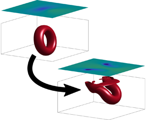
Figure 10 presents isosurfaces of vorticity magnitude at several time instances, revealing the evolution of the vortex ring as it interacts with the free surface. (A transient animation of this figure is provided as movie 1 in the supplementary material available at https://doi.org/10.1017/jfm.2022.529.) Initially, the vortex ring approaches the free surface under its own self-induced velocity (figure 10a). Then the upper portion of the vortex ring is flattened and stretched as it impinges upon the surface (figure 10b). This leads to large vorticity gradients at the free surface, so that vorticity from the upper portion of the vortex ring is diffused out of the fluid by viscous forces. As a result, the vortex ring becomes broken open near the free surface, leaving the open ends of the vortex ring attached to the free surface (figures 10c,d).

Figure 10. Isosurfaces of constant vorticity magnitude $|\omega |/(\varGamma _0/R_0^{2}) = 0.5$ at a range of dimensionless flow times, for the vortex ring/free surface interaction at $Re = 1570$, $Fr = 0.47$, $\alpha = 80^{\circ }$, $a/R = 0.35$ and $H/R = 2.5$. Contours of free-surface elevation, $\eta$ (displaced vertically for clarity) are also plotted.

While the isosurfaces of vorticity magnitude (figure 10) suggest that vortex connection has occurred, a change in topology of vorticity isosurfaces does not necessarily imply a change in the topology of vortex lines (Kida & Takaoka Reference Kida and Takaoka1994). In figure 11, vortex lines are plotted at two different times, before and after connection to the free surface has occurred. (An animation of this figure is provided in supplementary movie 2.) Initially, all vortex lines are closed loops (figure 11a,b); however, during the interaction, vortex lines are broken open near the free surface and become attached to the free surface (figure 11c,d). Isosurfaces of vorticity magnitude are also plotted in figure 11, demonstrating that, for the present flow, the geometries of vortex lines and vorticity isosurfaces are closely related.

Figure 11. Vortex lines, as well as isosurfaces of vorticity magnitude, (a,b) before and (c,d) after the free-surface connection. Vortex lines are colour coded, with red indicating closed loops, and blue indicating vortex lines that begin and terminate on the free surface. Both front (a,c) and side (b,d) views are provided. The dashed line in (a,c) indicates the symmetry plane ($y = 0$).

A colour plot of the free-surface displacement, $\eta$, is also provided in figure 10. As the vortex ring approaches the free surface, the surface is elevated ahead of the vortex ring, with a depression formed behind the vortex ring (figures 10a,b). As the vortex ring connects to the free surface, the free-surface depression splits into two surface dimples, which are located where the vortex ring is attached to the surface (figures 10c,d).

The qualitative aspects of vortex reconnection observed here compare fairly well to Zhang et al. (Reference Zhang, Shen and Yue1999); however, there are some key differences. First, in our results, the upper vortex core is flattened and stretched far more than in the Zhang et al. results. Second, in our simulations, some vorticity remains unattached to the free surface, which was not observed by Zhang et al. (Reference Zhang, Shen and Yue1999).

3.2. Two-fluid flow

The free-surface boundary conditions (2.9) and (2.10) are often used as an approximation for the air–water interface, where, due to the low density and viscosity of air, motion in the upper fluid (air) has little influence on the dynamics of the lower fluid (water). In this subsection, we consider the interaction between a vortex ring and a fluid–fluid interface, with density ratio $\rho _1/\rho _2 = 1000$ and viscosity ratio $\mu _1/\mu _2 = 100$, which are comparable to a water–air interface. Motion in the lower fluid is nearly identical to the free-surface case; the main difference between the free surface and the fluid–fluid interface is the appearance of vorticity in the upper fluid.

In figure 12, isosurfaces of vorticity magnitude are presented for the interaction between a vortex ring and a fluid–fluid interface, which can be compared to the free-surface flow plotted in figure 10. (A transient animation of this figure is provided in supplementary movie 3.) The behaviour of vorticity in the lower fluid is nearly identical to the free-surface flow, with the upper part of the vortex ring diffusing out of the lower fluid, and the open ends of the vortex ring attaching to the interface. This was confirmed in figure 6, which shows that the maximum vorticity in the lower fluid is not affected by the presence or absence of the upper fluid.

Figure 12. Isosurfaces of constant vorticity magnitude $|\omega |/(\varGamma _0/R_0^{2}) = 0.5$, at two dimensionless flow times, for the interaction between a vortex ring and a fluid–fluid interface, at $Re = 1570$, $Fr = 0.01$, $\alpha = 80$, $a/R_0 = 0.35$, $H/R_0 = 2.5$, $\rho _1/\rho _2 = 1000$ and $\mu _1/\mu _2 = 100$.

The most obvious difference between two-fluid and free-surface flows is the presence of vorticity in the upper fluid. This can be attributed to two factors: the creation of vorticity on the interface by tangential pressure gradients, and the transfer of vorticity between the upper and lower fluids. Vorticity appears first in the upper fluid before the reconnection has occurred (figure 12a), due to the creation of vorticity on the interface. During the reconnection process, vorticity from the upper part of the vortex ring is transferred from the lower fluid into the upper fluid (§ 4.4), so that after the reconnection, effectively the vortex ring passes through both fluids.

This is seen more clearly in figure 13, which plots vortex lines in both fluids, both before and after connection to the interface has occurred. (A transient animation of this figure is provided in supplementary movie 4.) Before the interaction, vortex lines in both fluids are closed loops, which lie entirely within a single fluid. After the interaction, vortex lines that attach to the interface are closed loops, passing through both fluids. Effectively, the upper part of the vortex ring has diffused into the upper fluid, and the vortex ring is contained in both fluids.

Figure 13. Vortex lines and isosurfaces of vorticity magnitude, (a) before and (b) after vortex connection to a fluid–fluid interface, at $\rho _1/\rho _2 = 1000$ and $\mu _1/\mu _2 = 100$. Vortex lines are colour coded, with red indicating closed loops that lie entirely within fluid 1, green indicating closed loops that lie entirely in fluid 2, and blue indicating vortex lines that pass through both fluids.

3.3. Interface vortex sheet

In several formulations of vorticity dynamics (Lundgren & Koumoutsakos Reference Lundgren and Koumoutsakos1999; Brøns et al. Reference Brøns, Thompson, Leweke and Hourigan2014; Terrington et al. Reference Terrington, Hourigan and Thompson2020, Reference Terrington, Hourigan and Thompson2022), a vortex sheet is included at the free surface, so that the total circulation is conserved. In three dimensions, Terrington et al. (Reference Terrington, Hourigan and Thompson2022) define the local density of vector circulation in the interface vortex sheet above a free surface as

(3.1)\begin{equation} \boldsymbol{\gamma} ={-}\hat{\boldsymbol{s}} \times \boldsymbol{u}. \end{equation}

By including the interface circulation in this manner, the total circulation is conserved (Terrington et al. Reference Terrington, Hourigan and Thompson2022). During the connection to the free surface, vorticity lost from the lower fluid is transferred into the interface vortex sheet (§ 4.2).

The interface vortex sheet also satisfies a generalised solenoidal property (Terrington et al. Reference Terrington, Hourigan and Thompson2022)

(3.2)\begin{equation} \boldsymbol{\nabla}_\parallel \boldsymbol{\cdot} \boldsymbol{\gamma} + \boldsymbol{\omega} \boldsymbol{\cdot} \hat{\boldsymbol{s}} = 0,\end{equation}

where $\boldsymbol {\nabla }_\parallel$ is the surface gradient operator (Wu Reference Wu1995). Equation (3.2) shows that vortex lines do not simply end on the free surface, but instead continue as circulation in the interface vortex sheet. This relationship is illustrated in figure 14, which plots vortex lines in the interface vortex sheet, as well as colour contours of surface-normal vorticity on the free surface. Before the connection has occurred, the surface-normal vorticity is zero, and the interface vortex sheet is divergence-free ($\boldsymbol {\nabla }_\parallel \boldsymbol {\cdot } \boldsymbol {\gamma } = 0$), so that vortex lines in the interface vortex sheet are all closed loops (figure 14a). However, after connection to the free surface has occurred, vortex lines in the interface vortex sheet are generated from regions of positive surface-normal vorticity, and end in regions of negative surface-normal vorticity (figure 14b).

Figure 14. Vortex lines in the interface vortex sheet (i.e. curves tangent to the interface circulation density, $\boldsymbol {\gamma }$), as well as colour contours of the surface-normal vorticity, at two different flow times.

Regions of high surface-normal vorticity, which act as sources and sinks for the interface vortex sheet, indicate regions where the vortex ring is attached to the free surface. This is shown in figure 15, which plots vortex lines in the fluid interior as well as in the interface vortex sheet. (A transient animation of this figure is provided in supplementary movie  5.) As vortex lines in the fluid interior connect to the free surface, they act as sources or sinks of circulation in the free-surface vortex sheet. In this sense, vortex lines do not end on the free surface, but continue as vortex lines in the interface vortex sheet. After the connection to the free surface, the vortex ring remains a closed loop, but with part of the vortex ring attached to the free surface. Essentially, the upper part of the vortex ring has diffused out of the fluid, and is now contained in the interface vortex sheet.

Figure 15. Vortex lines in the fluid as well as in the interface vortex sheet, both (a) before and (b) after vortex reconnection has occurred. Vortex lines are colour coded, with red indicating closed loops, while blue indicates vortex lines that begin and terminate on the free surface.

Comparing figures 15 and 13 reveals several similarities between the interface vortex sheet above a free surface, and the vorticity field above a fluid–fluid interface. Before the interaction, vortex lines in the upper fluid are closed loops, as are the vortex lines in the interface vortex sheet. After the interaction, vortex lines in the interface vortex sheet begin and end at points where the vortex ring attaches to the free surface, as do vortex lines in the upper fluid for the two-fluid case. In this sense, the free-surface vortex sheet can be interpreted as an approximation for the vorticity that would be found above an air–water interface.

4.1. Vorticity dynamics

Taking the curl of the momentum equation yields a transport equation for vorticity (the Helmholtz equation). For an incompressible Newtonian fluid, this equation is expressed as

(4.1)\begin{equation} \frac{\partial {\omega}}{\partial {t}} + \boldsymbol{u} \boldsymbol{\cdot} \boldsymbol{\nabla} \boldsymbol{\omega} = \boldsymbol{ \omega} \boldsymbol{\cdot} {\boldsymbol{\nabla}}\boldsymbol{u} + \nu\,{\nabla}^{2} \boldsymbol{\omega}.\end{equation}

Equation (4.1) reveals three relevant dynamical processes for the evolution of the vorticity field: advection ($\boldsymbol {u} \boldsymbol {\cdot } \boldsymbol {\nabla } \boldsymbol {\omega }$), vortex stretching/tilting ($\boldsymbol {\omega } \boldsymbol {\cdot }\boldsymbol {\nabla } \boldsymbol {u}$) and viscous diffusion ($\nu \, {\nabla }^{2} \boldsymbol {\omega }$). If this expression is integrated across a control volume ($V$), then these dynamical processes can be interpreted as boundary fluxes (Terrington et al. Reference Terrington, Hourigan and Thompson2022):

(4.2)\begin{equation} \frac{\mathrm{d} {}}{\mathrm{d} t} \int_V \boldsymbol{\omega} \,\mathrm{d} V = \oint_{\partial V} \boldsymbol{\omega} (\boldsymbol{v}^{b} -\boldsymbol{u}) \boldsymbol{\cdot} \hat{\boldsymbol{n}} \,\mathrm{d} S + \oint_{\partial V} (\boldsymbol{\omega} \boldsymbol{\cdot} \hat{\boldsymbol{n}})\boldsymbol{u}\,\mathrm{d} S - \oint_{\partial V} \nu \hat{\boldsymbol{n}} \times (\boldsymbol{\nabla} \times \boldsymbol{\omega}) \,\mathrm{d} S,\end{equation}

where $\partial V$ is the boundary surface of $V$, $\hat {\boldsymbol {n}}$ is the outward-oriented unit normal to $\partial V$, and $\boldsymbol {v}^{b}$ is the velocity of the control-volume boundary. From left to right, terms on the right-hand side of (4.2) represent the effects of advection, vortex stretching/tilting and viscous diffusion as boundary fluxes.

Now, the form of the viscous boundary flux in (4.2) is not unique. Here, we have used the Lyman (Reference Lyman1990) definition, $\boldsymbol {\sigma } = \nu \hat {\boldsymbol {n}} \times (\boldsymbol {\nabla } \times \boldsymbol {\omega })$, rather than the original definition proposed by Lighthill (Reference Lighthill1963), $\boldsymbol {\sigma }' = - \nu \hat {\boldsymbol {n}} \boldsymbol {\cdot } \boldsymbol {\nabla } \boldsymbol {\omega }$. When integrated across a control volume, both definitions yield the same rate of change of vorticity, so either definition may be used in (4.2). Terrington, Hourigan & Thompson (Reference Terrington, Hourigan and Thompson2021) have demonstrated several advantages to using Lyman's definition. Of particular relevance to the present work, Lyman's definition was found to provide a more elegant interpretation of the connection between antiparallel vortex filaments in the fluid interior. In the present article, we also show that Lyman's definition also provides a more elegant interpretation of the mechanism behind the attachment of vortex filaments to the free surface during the connection process.

The shear-free boundary condition (2.9) can be written as a boundary condition for the surface-tangential vorticity on the free surface (Longuet-Higgins Reference Longuet-Higgins1998; Peck & Sigurdson Reference Peck and Sigurdson1998; Terrington et al. Reference Terrington, Hourigan and Thompson2022):

(4.3)\begin{equation} \boldsymbol{\omega}_{{\parallel},1} ={-}{2}\hat{\boldsymbol{s}}\times (\boldsymbol{\nabla}_{{\parallel}}(\boldsymbol{u}_1 \boldsymbol{\cdot} \hat{\boldsymbol{s}}) + \boldsymbol{u}_1 \boldsymbol{\cdot} {\boldsymbol{\mathsf{K}}}),\end{equation}

where $\boldsymbol {\omega }_{\parallel } = \boldsymbol {\omega } - (\hat {\boldsymbol {s}} \boldsymbol {\cdot } \boldsymbol {\omega }) \hat {\boldsymbol {s}}$ is the surface-parallel vorticity on the free surface, $\hat {\boldsymbol {s}}$ is the unit normal to the interface, directed out of fluid 1, $\boldsymbol {\nabla }_\parallel$ is the surface gradient operator (Wu Reference Wu1995), and ${\boldsymbol{\mathsf{K}}} = \boldsymbol {\nabla }_{\parallel } \hat {\boldsymbol {s}}$ is the surface curvature tensor. The viscous flux of vorticity at the free surface results in the diffusion of vorticity either into or out of the fluid, in order to satisfy this boundary condition (Terrington et al. Reference Terrington, Hourigan and Thompson2022). At low Froude numbers, the right-hand side of (4.3) is small, and the vorticity on the free surface is close to zero. However, at higher Froude numbers, distortion of the free surface leads to the appearance of secondary vorticity on the free surface (Gharib & Weigand Reference Gharib and Weigand1996; Zhang et al. Reference Zhang, Shen and Yue1999).

4.2. Control-volume analysis

To examine the mechanisms leading to the loss of vorticity from the fluid, we consider the control volume depicted in figure 16. The outer boundary of $V_1$ is divided into two portions: $I$ is the part that lies on the free surface, while $\partial V_1$ is the part in the fluid interior. The vector $\hat {\boldsymbol {n}}$ is the unit normal to $\partial V_1$, while $\hat {\boldsymbol {s}}$ is the unit normal to the free surface.

Figure 16. Control volume $V_1$ used in this analysis. The boundary of $V_1$ includes a portion on the free surface ($I$) and a portion in the fluid interior ($\partial V_1$). The surface $I$ is bounded by the closed curve $\partial I$. The unit normal to $I$ is $\hat {\boldsymbol {s}}$, while $\hat {\boldsymbol {n}}$ is the unit normal to $\partial V$.

In this subsection, we consider the volume integral of vorticity

(4.4)\begin{equation} \boldsymbol{\varGamma}_1 = \int_{V_1}\boldsymbol{\omega}_1 \,\mathrm{d} V, \end{equation}

which we have termed the ‘vector circulation’ (Terrington et al. Reference Terrington, Hourigan and Thompson2021, Reference Terrington, Hourigan and Thompson2022). We also consider the total vector circulation contained in the interface vortex sheet,

(4.5)\begin{equation} \boldsymbol{\varGamma}_{\gamma} = \int_{I_1} \boldsymbol{\gamma}\,\mathrm{d} S. \end{equation}

While both $\boldsymbol {\varGamma }_1$ and $\boldsymbol {\varGamma }_\gamma$ are vector-valued quantities, due to flow symmetry only the spanwise components ($\varGamma _{1,y}$ and $\varGamma _{\gamma,y}$) are non-zero. The time histories of both these quantities are plotted in figure 17(a). The net spanwise vorticity in the fluid is zero initially, due to the symmetry of the vortex ring. However, $\varGamma _{1,y}$ increases throughout the interaction, as negative vorticity from the upper part of the vortex ring diffuses out of the fluid. The loss of negative spanwise vorticity from the fluid is balanced by an approximately equal increase in negative circulation found in the vortex sheet, so that the total circulation ($\varGamma _{1,y} + \varGamma _{\gamma,y}$) remains approximately constant.

Figure 17. (a) Time history of the spanwise component of vector circulation in the fluid ($\varGamma _{1,y}$) and in the interface vortex sheet ($\varGamma _{\gamma,y}$). (b) Comparison between the rate of change of spanwise vorticity, and the viscous and vortex stretching terms from (4.6).

Using (4.2), we construct the following expression for the rate of change of vorticity in $V_1$:

(4.6)\begin{equation} \frac{\mathrm{d} {\boldsymbol{\varGamma}_1}}{\mathrm{d} t} ={-}\int_I \nu \hat{\boldsymbol{s}} \times (\boldsymbol{\nabla} \times \boldsymbol{\omega}) \,\mathrm{d} S + \int_I (\boldsymbol{\omega} \boldsymbol{\cdot} \hat{\boldsymbol{s}}) \boldsymbol{u} \,\mathrm{d} S,\end{equation}

where we have assumed that vorticity fluxes across $\partial V_1$ are negligible. This equation indicates the two mechanisms that contribute to the rate of change of vorticity in the fluid: the viscous boundary flux $F_{\nu } =\int _I \nu \hat {\boldsymbol {s}} \times (\boldsymbol {\nabla } \times \boldsymbol {\omega }) \,\mathrm {d} S$, and the vortex stretching/tilting flux $F_{st} = \int _I (\boldsymbol {\omega } \boldsymbol {\cdot } \hat {\boldsymbol {s}}) \boldsymbol {u}\,\mathrm {d} S$.

The rate of change of circulation above the free surface is given by the expression (Terrington et al. Reference Terrington, Hourigan and Thompson2022)

(4.7)\begin{equation} \frac{\mathrm{d} {\boldsymbol{\varGamma}_\gamma}}{\mathrm{d} t} = \int_I \nu\hat{\boldsymbol{s}} \times (\boldsymbol{\nabla} \times \boldsymbol{\omega})\,\mathrm{d} S - \int_I (\boldsymbol{\omega} \boldsymbol{\cdot} \hat{\boldsymbol{s}}) \boldsymbol{u} \,\mathrm{d} S + \oint_{\partial I} \left[\frac{p_1}{\rho_1} + \phi_g + \frac{1}{2}\, \boldsymbol{u}_1 \boldsymbol{\cdot} \boldsymbol{u}_1 \right] \mathrm{d} s.\end{equation}

The first two terms are equal and opposite to the free-surface flux terms in (4.6), so that the effects of viscous diffusion and vortex stretching/tilting act to transfer circulation between the fluid interior and the interface vortex sheet. Any loss of negative circulation is balanced by an equal gain of negative circulation in the interface vortex sheet.

Combining (4.7) and (4.6), we have

(4.8)\begin{equation} \frac{\mathrm{d} {}}{\mathrm{d} t} (\boldsymbol{\varGamma}_{1} + \boldsymbol{\varGamma}_\gamma )= \oint_{\partial I} \left[\frac{p_1}{\rho_1} + \phi_g + \frac{1}{2}\,\boldsymbol{u}_1 \boldsymbol{\cdot} \boldsymbol{u}_1 \right] \mathrm{d} s,\end{equation}

which includes several boundary source terms that represent the generation of interface circulation by tangential pressure gradients ($p_1/\rho _1$) or gravitational forces ($\phi _g$), as well as the advection of circulation along the interface ($\boldsymbol {u}_1 \boldsymbol {\cdot } \boldsymbol {u}_1$). For the control volume used in this analysis, these boundary terms are small but non-zero, leading to small oscillations in the total circulation. However, these terms will approach zero if $\partial I$ is positioned sufficiently far from the vortex ring, and the total circulation will be conserved.

The time histories of the viscous and vortex stretching/tilting fluxes, as well as the rate of change of spanwise vorticity, are plotted in figure 17(b). Initially, the increase in $\varGamma _{1,y}$ (and decrease in $\varGamma _{\gamma,y}$) is due to the viscous flux of vorticity out of the fluid. During the initial stage of the connection process, negative spanwise vorticity from the upper part of the vortex ring is brought near the free surface. At low Froude numbers, (4.3) requires the tangential vorticity at the free surface to be small, leading to a large gradient of spanwise vorticity ($\partial \omega _y/\partial z$) on the free surface. This vorticity gradient drives the viscous flux of vorticity out of the fluid and into the free-surface vortex sheet.

While the viscous flux dominates the initial loss of negative circulation from the fluid, the vortex stretching term ($F_{st}$) becomes the dominant mechanism in the later portion of this interaction. An interpretation of the vortex stretching/tilting flux was presented in (Terrington et al. Reference Terrington, Hourigan and Thompson2022). Eyink (Reference Eyink2008) gives a simple proof for the expression

(4.9)\begin{equation} \boldsymbol{\varGamma}_1 = \int_{V_1} \boldsymbol{\omega} \,\mathrm{d} V = \oint_{\partial V_1} \boldsymbol{x} (\boldsymbol{\omega} \boldsymbol{\cdot} \hat{\boldsymbol{n}}) \,\mathrm{d} S + \oint_{I} \boldsymbol{x} (\boldsymbol{\omega} \boldsymbol{\cdot} \hat{\boldsymbol{s}}) \,\mathrm{d} S,\end{equation}

where $\boldsymbol {x}$ is the position vector, which (assuming that $\boldsymbol {\omega } \boldsymbol {\cdot } \hat {\boldsymbol {n}} = 0$ on $\partial V_1$) shows that the total vorticity in $V_1$ is determined completely by the locations where vortex filaments are attached to the free surface. The vortex stretching flux ($\boldsymbol {u} (\boldsymbol {\omega } \boldsymbol {\cdot } \hat {\boldsymbol {s}})$) can be interpreted as representing the advection of surface-normal vorticity in the free surface. This changes the locations where vortex filaments attach to the surface, therefore requiring a change to the total vorticity in the fluid.

This is illustrated in figure 18, where a positive $F_{st}$ requires surface-attached vorticity to be carried away from the symmetry plane by advection. As a result, new spanwise vorticity must be generated by vortex stretching in the fluid interior, since vortex lines cannot end inside the fluid. Moreover, an equal quantity of opposite-signed circulation must be created in the interface vortex sheet, in order to satisfy the generalised solenoidal condition (3.2).

Figure 18. Illustration of the vortex stretching/tilting flux $\boldsymbol {u}(\boldsymbol {\omega } \boldsymbol {\cdot } \hat {\boldsymbol {s}})$ from (4.6). This term can be interpreted as representing the advection of vortex filaments in the free surface, which must correspond to the creation of spanwise vorticity by vortex stretching in the fluid interior. An equal and opposite quantity of circulation is also created in the interface vortex sheet, so that the total spanwise circulation is conserved.

4.3. Control-surface analysis

The dynamical mechanisms leading to the connection of vorticity to the free surface can be understood by considering the behaviour of circulation in both the symmetry plane ($y = 0$) and the free surface. Contours of the spanwise vorticity ($\omega _y$) in the symmetry plane, and of surface-normal vorticity ($\boldsymbol {\omega } \boldsymbol {\cdot } \hat {\boldsymbol {s}}$) in the free surface, are presented in figure 19, both before and after reconnection has occurred. (A transient animation of this figure is provided in supplementary movie  6.) This figure demonstrates one of the main features of vortex connection to the free surface: the loss of negative spanwise vorticity from the symmetry plane (which signifies the breaking open of vortex filaments near the free surface), and the appearance of new vorticity in the free surface (indicating the attachment of vortex lines to the free surface).

Figure 19. Contours of spanwise vorticity ($\omega _y$) in the symmetry plane ($y= 0$), and of surface-normal vorticity ($\boldsymbol {\omega } \boldsymbol {\cdot } \hat {\boldsymbol {s}}$) in the free surface, both (a) before and (b) after the free surface connection has occurred. Contours of dimensionless vorticity are plotted for $\omega /(\varGamma _0/R_0^{2}) = \ldots,-1.25,-0.75,-0.25,0.25,0.75,1.25, \ldots$.

To quantify the reconnection process, we consider the circulation contained in the system of control surfaces illustrated in figure 20: $S_1$ is the symmetry plane; $I_1$ is the portion of the free surface where $y<0$; and $I_2$ is the portion of the free surface where $y>0$. The time history of circulation in each reference surface is plotted in figure 21(a), where $\varGamma_{I_1}, \varGamma_{I_2}$ and $\varGamma_{S_1}$ are the circulations contained in surfaces $I_1,\, I_2$ and $S_1$, respectively. As the upper part of the vortex ring diffuses out of the free surface, the circulation in $S_1$ increases (becomes more positive), and this is balanced by an equal gain of negative circulation in $I_1$, and of positive circulation in $I_2$.

Figure 20. Illustration of the control surfaces $S_1$, $I_1$ and $I_2$ used in this investigation. These surfaces share a common boundary – the connection line, $C$ – and the remaining portions of the boundaries are denoted $\partial S_1$, $\partial I_1$ and $\partial I_2$, respectively.

Figure 21. (a) Time history of the circulation in the surfaces $I_1$, $I_2$ and $S_1$, as well as of the interface circulation $\varGamma _\gamma$. (b) A comparison between the rate of change of circulations and the viscous boundary flux $F_\nu$, defined in (4.11).

The transfer of circulation between the symmetry plane and the free surface is related closely to the top topological changes to vortex lines observed in figure 11. Two kinds of vortex line topology are present in this flow: closed loops and open filaments. Loop-type vortex filaments pass through the symmetry plane twice, so the net spanwise circulation in the symmetry plane due to a closed vortex filament is zero. As the initial vortex ring contains only closed filaments, the initial circulations in $S_1$, $I_1$ and $I_2$ are all zero. Open filaments, however, begin on $I_2$, pass through $S_1$ once, and end on $I_1$, providing an equal magnitude of positive circulation in $I_2$, and negative circulation in $S_1$ and $I_1$. The changes in circulation shown in figure 21 therefore describe the opening of vortex loops, and the attachment of open vortex lines to the free surface.

In figure 21 we also plot the interface circulation contained in the connection line ($C$):

(4.10)\begin{equation} \varGamma_{\gamma} = \int_C \boldsymbol{\gamma}\boldsymbol{\cdot} \hat{\boldsymbol{b}}\,\mathrm{d} s = \int_C - \boldsymbol{u}_1 \boldsymbol{\cdot} \mathrm{d} \boldsymbol{s}. \end{equation}

The loss of negative circulation from $S_1$ is also balanced by an equal gain of negative circulation in $C$, so that the total circulation $\varGamma _{S_1} + \varGamma _{\gamma }$ is constant. Effectively, the upper part of the vortex ring has been transferred into the interface vortex sheet, and vortex lines intersect the symmetry plane twice: once as vorticity in the fluid interior, and once as circulation in the interface vortex sheet.

The rate of change of circulation in each surface is given by the fluxes of vorticity across the boundary of each surface. Assuming that the outer boundary curves ($\partial S_1$, $\partial I_1$ and $\partial I_2$) are sufficiently far from the vortex ring, fluxes across these surfaces are negligible, and the circulation in each surface can change only due to vorticity fluxes along the connection line $C$. Then the rate of change of circulation in each surface is given by (Terrington et al. Reference Terrington, Hourigan and Thompson2022)

(4.11a)\begin{gather} \frac{\mathrm{d} {\varGamma_{S_1}}}{\mathrm{d} t} = \frac{\mathrm{d} {}}{\mathrm{d} t}\int_{S_1} \boldsymbol{\omega} \boldsymbol{\cdot} \hat{\boldsymbol{n}} \,\mathrm{d} S = F_\nu, \end{gather}

(4.11b)\begin{gather}\frac{\mathrm{d} {\varGamma_{I_1}}}{\mathrm{d} t} = \frac{\mathrm{d} {}}{\mathrm{d} t}\int_{I_1} \boldsymbol{\omega} \boldsymbol{\cdot} \hat{\boldsymbol{s}}\,\mathrm{d} S ={-}F_\nu, \end{gather}

(4.11c)\begin{gather}\frac{\mathrm{d} {\varGamma_{I_2}}}{\mathrm{d} t} = \frac{\mathrm{d} {}}{\mathrm{d} t}\int_{I_2} \boldsymbol{\omega} \boldsymbol{\cdot} \hat{\boldsymbol{s}}\,\mathrm{d} S = F_\nu, \end{gather}

(4.11d)\begin{gather}\frac{\mathrm{d} {\varGamma_\gamma}}{\mathrm{d} t} ={-}F_{\nu} + \left[\frac{p_1}{\rho_1} \right]_{(b-a)} + \left [\phi_g\right]_{(b-a)} + \frac{1}{2}\left[\boldsymbol{u}_1 \boldsymbol{\cdot} \boldsymbol{u}_1 \right]_{(b-a)}, \end{gather}

(4.11e)\begin{gather}F_\nu ={-}\int_C [\hat{\boldsymbol{s}} \times (\boldsymbol{\nabla} \times \boldsymbol{\omega}) ]\boldsymbol{\cdot} \hat{\boldsymbol{b}}\,\mathrm{d} s, \end{gather}

where $F_\nu$ is the viscous flux of vorticity across the connection line ($C$), and subscript $(b-a)$ indicates the difference in some quantity between the endpoints of $C$ ($\theta _{(b-a)} = \theta _b - \theta _a$).

Equations (4.11) attribute the loss of circulation from the symmetry plane, and the gain of circulation in $I_1$ and $I_2$, to the viscous flux of vorticity across the connection line. Importantly, the loss of circulation from the symmetry plane represents the breaking open of vortex filaments, while the appearance of vorticity in the free surface indicates the attachment of these vortex lines to the free surface. Equations (4.11) show that these processes always occur simultaneously – which must be the case, since vortex filaments cannot end in the fluid interior – and are driven by the same physical process: the viscous boundary flux.

First, consider the loss of spanwise vorticity from the symmetry plane, which is illustrated by the contour plots of spanwise vorticity presented in figure 22. Initially, the vortex ring approaches the free surface under its own self-induced velocity. As the upper vortex core interacts with the free surface, it is flattened and stretched (figures 22b,c), resulting in a strong gradient of spanwise vorticity at the free surface ($\partial \omega _y/\partial z$). According to (4.11), this results in a viscous flux of spanwise vorticity out of the symmetry plane, so that most of the negative vorticity in the upper vortex core is diffused out of the fluid (figure 22d).

Figure 22. Contours of spanwise vorticity ($\omega _y$) in the symmetry plane ($y= 0$) at several times throughout the interaction. The colourmap and contour levels are the same as in figure 19.

According to (4.11d), $F_\nu$ also contributes to the rate of change of interface circulation, so the circulation lost from $S_1$ is transferred into the interface vortex sheet. Additional boundary terms also appear in this equation, representing the generation of interface circulation by tangential pressure gradients and body forces, as well as the advection of interface circulation along the surface. If the boundary points, $a$ and $b$, are sufficiently far from the vortex ring, these terms approach zero, and the total circulation in the symmetry plane – including vorticity in the fluid, and circulation in the interface vortex sheet – is constant.

Now we consider the appearance of vorticity in the free surface, which is illustrated by the contours of surface-normal vorticity presented in figure 23. Initially, there is almost no vorticity in the free surface (figure 23a). However, during the interaction, positive vorticity appears in $I_2$, while negative vorticity appears in $I_1$. Equations (4.11) attribute this to the viscous vorticity flux at the connection line ($y = 0$), which is due to the same vorticity gradients that lead to the loss of circulation from the symmetry plane (primarily the gradient of spanwise vorticity, $\partial \omega _y/\partial z$). In other words, the flux of negative spanwise vorticity out of the symmetry plane is associated with an equal flux of negative surface-normal vorticity into $I_1$, and positive surface-normal vorticity into $I_2$. This is necessary to ensure that the kinematic condition that vortex lines do not end in the fluid interior is satisfied.

Figure 23. Contours of surface-normal vorticity ($\boldsymbol {\omega } \boldsymbol {\cdot } \hat {\boldsymbol {s}}$) in the free surface at several times throughout the interaction. The colourmap and contour levels are the same as in figure 19. The dashed line indicates the connection line ($y=0$), which is the shared boundary of the surfaces $I_1$, $I_2$ and $S_1$.

4.4. Two-fluid flows

For two-fluid flows, the vorticity balance is similar to the free-surface case considered in §§ 4.2 and 4.3, although vorticity is transferred into the upper fluid, rather than into the interface vortex sheet. For the control-volume analysis, we use the system of control volumes shown in figure 24(a), where $V_1$ and $V_2$ are control volumes in fluids $1$ and $2$, respectively. The two volumes share a common boundary, $I$, on the interface, while $\partial V_1$ and $\partial V_2$ are the boundary surfaces in the fluid interior. Finally, $\partial I$ is the outer boundary curve of $I$.

Figure 24. System of (a) control volumes, and (b) control surfaces used to analyse the vortex ring connection to a fluid–fluid interface. The volumes $V_1$ and $V_2$ are control volumes in the lower and upper fluids, respectively. Also, $S_1$ and $S_2$ are the portions of the symmetry plane in the upper and lower fluids, respectively, while $I_1$ and $I_2$ are surfaces that lie in the interface.

For the system of control volumes shown in figure 24(a), the rate of change of vorticity is given by (Terrington et al. Reference Terrington, Hourigan and Thompson2022)

(4.12)\begin{equation} \frac{\mathrm{d} {}}{\mathrm{d} t}\left(\boldsymbol{\varGamma}_1+\boldsymbol{\varGamma}_2\right) ={-}\int_{I} \left[\!\left[\nu \hat{\boldsymbol{s}} \times (\boldsymbol{\nabla} \times \boldsymbol{\omega})\right]\!\right]\mathrm{d} S = \oint_{\partial I} \left[\!\left[\frac{p}{\rho} \right]\!\right] \mathrm{d} \boldsymbol{s},\end{equation}

where we have assumed that the fluxes of vorticity across the outer boundary ($\partial V$) are negligible. Equation (4.12) indicates that the total vorticity within the system can change only by the generation of vorticity by tangential pressure gradients on the interface $\left (\left[\!\left[ p/\rho \right]\!\right] \right )$. Vorticity generated on the interface is diffused immediately into the fluid by viscous forces, and the net viscous flux of vorticity out of the interface $\left (\left[\!\left[ \nu \hat {\boldsymbol {s}} \times (\boldsymbol {\nabla } \times \boldsymbol {\omega })\right]\!\right] \right )$ is equal to the vorticity creation rate. Importantly, if the outer boundary curve $\partial I$ is sufficiently far from the vortex ring, then the net vorticity creation will be zero. Generation of vorticity by local pressure gradients on some section of the interface may still occur, but this will be balanced by the creation of opposite-signed vorticity elsewhere.

The time history of total spanwise vorticity in each fluid is plotted in figure 25(b), which can be compared to the free-surface case in figure 17(a). As the upper portion of the vortex ring diffuses out of the fluid, there is a loss of negative spanwise vorticity from the lower fluid. This is balanced approximately by an equal gain of negative vorticity in the upper fluid, so that the total vorticity in both fluids remains approximately constant. Effectively, negative vorticity lost from the lower fluid is transferred into the upper fluid. This is similar to the free-surface case, where vorticity lost from the lower fluid is transferred into the interface vortex sheet.

Figure 25. Time histories of (a) the circulation in both the symmetry plane ($S_1$ and $S_2$) and the interface ($I_1$ and $I_2$). (b) The spanwise component of vector circulation in each fluid ($\varGamma _{1,y}$ and $\varGamma _{2,y}$), for the interaction between a vortex ring and a fluid-fluid interface.

Note, however, that significant oscillations in the total vorticity are present in figure 25(b), which are due to the pressure generation term. This is confirmed in figure 26(b), which plots the various terms in (4.12) and demonstrates clearly that the oscillations in total circulation are due to pressure gradients on the interface. The pressure term will decrease to zero as the size of the control volume is increased, and the total circulation will be constant.

Figure 26. The net rate of change of (a) total circulation in the symmetry plane ($\varGamma_{S_1} + \varGamma_{S_2}$), and (b) spanwise component of vector circulation in both fluids ($\varGamma _{1,y}+\varGamma _{2,y}$), as well as the net vorticity generation by pressure gradients ($S_p$ and $S_{p,y}$) and the net viscous flux of vorticity out of the interface ($F_{\nu,1}+F_{\nu,2}$).

For the control-surface analysis, we use the system of control surfaces in figure 24(b), which includes the parts of the symmetry plane in fluid 1 ($S_1$) and fluid 2 ($S_2$), as well as the surfaces $I_1$ and $I_2$ on the interface. The rate of change of circulation in each surface is given by the viscous flux of vorticity along the connection line:

(4.13a)\begin{gather} \frac{\mathrm{d} {\varGamma_{S_{1}}}}{\mathrm{d} t} = \frac{\mathrm{d} {}}{\mathrm{d} t}\int_{S_1} \boldsymbol{\omega} \boldsymbol{\cdot} \hat{\boldsymbol{n}} \,\mathrm{d} S = F_{\nu,1}, \end{gather}

(4.13b)\begin{gather}\frac{\mathrm{d} {\varGamma_{S_{2}}}}{\mathrm{d} t} = \frac{\mathrm{d} {}}{\mathrm{d} t}\int_{S_1} \boldsymbol{\omega} \boldsymbol{\cdot} \hat{\boldsymbol{n}} \,\mathrm{d} S = F_{\nu,2}, \end{gather}

(4.13c)\begin{gather}\frac{\mathrm{d} {\varGamma_{I_{1}}}}{\mathrm{d} t} = \frac{\mathrm{d} {}}{\mathrm{d} t}\int_{S_1} \boldsymbol{\omega} \boldsymbol{\cdot} \hat{\boldsymbol{s}} \,\mathrm{d} S ={-}F_{\nu,1}, \end{gather}

(4.13d)\begin{gather}\frac{\mathrm{d} {\varGamma_{I_{2}}}}{\mathrm{d} t} = \frac{\mathrm{d} {}}{\mathrm{d} t}\int_{S_1} \boldsymbol{\omega} \boldsymbol{\cdot} \hat{\boldsymbol{s}} \,\mathrm{d} S = F_{\nu,1}, \end{gather}

(4.13e)\begin{gather}F_{\nu,1} = \int_C -[\hat{\boldsymbol{s}} \times (\boldsymbol{\nabla} \times \boldsymbol{\omega}_1) ]\boldsymbol{\cdot} \hat{\boldsymbol{b}}\,\mathrm{d} s, \end{gather}

(4.13f)\begin{gather}F_{\nu,2} = \int_C [\hat{\boldsymbol{s}} \times (\boldsymbol{\nabla} \times \boldsymbol{\omega}_2) ]\boldsymbol{\cdot} \hat{\boldsymbol{b}}\,\mathrm{d} s, \end{gather}

where $F_{\nu,1}$ is the flux of vorticity into fluid 1, and $F_{\nu,2}$ is the flux of vorticity into fluid 2. Moreover, the net rate of change of circulation in the symmetry plane is given by

(4.14) \begin{equation} \frac{\mathrm{d} {}}{\mathrm{d} t}(\varGamma_{S_{1}}+\varGamma_{S_{2}}) = \left[\!\left[ \frac{p}{\rho} \right]\!\right]_{(b-a)} = F_{\nu,1} + F_{\nu,2},\end{equation}

which changes only due to the net generation of vorticity by pressure gradients on the interface. If the boundary points $a$ and $b$ are positioned sufficiently far from the vortex ring, then the pressure term will be zero, and the total circulation will be conserved.

The time history of circulation in each reference surface is plotted in figure 25(a). As in the free-surface case (figure 21a), the viscous flux ($F_{\nu,1}$) is responsible for the loss of circulation from the lower fluid ($S_1$), as well as the attachment of surface-normal vorticity to the free surface. Moreover, the loss of circulation from $S_1$ is balanced by an equivalent flux of circulation into $S_2$ ($F_{\nu,2}$), so the total circulation in the symmetry plane ($\varGamma _{S_{1}}+\varGamma _{S_{2}}$) is approximately constant. This resembles the free-surface case, where the loss of circulation from the fluid is balanced by the increase in circulation contained in the interface vortex sheet.

As with the control-volume analysis, significant oscillations are observed in the total circulation in the symmetry plane ($\varGamma _{S_{1}}+\varGamma _{S_{2}}$), due to the creation of vorticity by pressure gradients. The various terms from (4.14) are plotted in figure 26(a), which confirms that the oscillations in total circulation are due to the pressure generation term. Once again, as the control-surface boundary is moved further from the vortex ring, these oscillations will decrease, and the total circulation will be constant.

The similarities between the circulation balances for free-surface and two-fluid flows suggests that the interface vortex sheet above a free surface plays a similar role to the vorticity that would be found above an air–water interface. For the two-fluid case, the loss of vorticity from the lower fluid is balanced by an equal increase in the vorticity contained in the upper fluid. For the free-surface case, the loss of vorticity from the lower fluid is instead balanced by an increase in the circulation contained in the interface vortex sheet.

4.5. Mechanism of vortex connection

The analysis considered in this section suggests a novel interpretation of the vortex connection to a free surface. In this subsection, we compare this interpretation to the previous mechanism proposed by Gharib & Weigand (Reference Gharib and Weigand1996) and Zhang et al. (Reference Zhang, Shen and Yue1999).

A sketch of the vortex connection mechanism is presented in figure 27(a). As the upper portion of the vortex ring interacts with the free surface, the gradient of spanwise vorticity at the free surface ($\partial \omega _y/\partial z$) results in a viscous flux of surface-tangential vorticity out of the fluid. The upper part of the vortex ring diffuses out of the fluid, and into the interface vortex sheet. The flux of spanwise vorticity out of the fluid is accompanied by the diffusion of opposite-signed surface-normal vorticity away from the connection line, along the free surface, which results in the attachment of vortex lines to the free surface.

Figure 27. A comparison between (a) our interpretation of the vortex attachment process, and (b) the mechanism proposed by Zhang et al. (Reference Zhang, Shen and Yue1999). In our description, the attachment of vorticity to the free surface is attributed to the diffusion of surface-normal vorticity along the free surface, and away from the connection line, while in the Zhang et al. (Reference Zhang, Shen and Yue1999) interpretation, this is attributed to the diffusion of surface-normal vorticity from the fluid interior.

Under this interpretation, the attachment of vortex filaments to the free surface is attributed directly to the viscous flux of spanwise vorticity out of the fluid. Therefore, the mechanism that drives the loss of spanwise vorticity from the fluid is also responsible for the attachment of vortex filaments to the free surface. This is beneficial, since the divergence-free property of the vorticity field – where vortex lines cannot end in the fluid interior – requires that the circulation lost from the symmetry plane must be gained in the free surface. Our interpretation illustrates clearly how this condition is enforced.

This interpretation of the vortex attachment mechanism differs substantially from previous interpretations (Rood Reference Rood1994a,Reference Roodb; Gharib & Weigand Reference Gharib and Weigand1996; Zhang et al. Reference Zhang, Shen and Yue1999). While Rood (Reference Rood1994a) describes in great detail the mechanisms by which surface-tangential vorticity diffuses out of the fluid, he does not ascribe the attachment of vorticity to the surface to any particular physical process. Instead, he states that ‘a portion of the closed vortex loop fluxes out of the fluid, leaving the remainder of the loop with ends terminating at the free surface’ (Rood Reference Rood1994a) – thereby treating the free-surface attachment as a kinematic consequence of the loss of tangential vorticity from the fluid.

While both Gharib & Weigand (Reference Gharib and Weigand1996) and Zhang et al. (Reference Zhang, Shen and Yue1999) also attribute the breaking open of vortex filaments to the diffusion of surface-tangential vorticity out of the fluid, they attribute the attachment of vortex filaments to the surface to the diffusion of surface-normal vorticity towards the free surface from the fluid interior, as illustrated in figure 27(b). The side regions of the vortex ring contain surface-normal vorticity, which is enhanced by vortex stretching and tilting. This surface-normal vorticity is then transported to the free surface by viscous diffusion. Unlike the surface-parallel vorticity, which diffuses out of the fluid to satisfy the shear-free condition, the flux of surface-normal vorticity out of the fluid is small, and the surface-normal vorticity instead remains attached to the surface. Importantly, this interpretation treats the loss of spanwise vorticity from the fluid and the attachment of vortex lines to the free surface as different dynamical processes, and it is unclear why the exact quantity of circulation lost from the symmetry is gained in the free surface.

The difference between the interpretation provided by Zhang et al. (Reference Zhang, Shen and Yue1999) and our proposed interpretation is also demonstrated in figure 28, which is inspired by figure 24 of Zhang et al. (Reference Zhang, Shen and Yue1999). Zhang et al. attribute the appearance of surface-normal vorticity ($\omega _z$) in the free surface to viscous diffusion of surface-normal vorticity from the fluid interior (red dotted line in figure 28). Under the proposed interpretation, this is instead attributed to the diffusion of surface-normal vorticity along the free surface (solid blue line in figure 28), which occurs as a direct consequence of the diffusion of surface-tangential vorticity ($\omega _y$) out of the fluid. All other aspects of the interpretation are unchanged, as indicated by solid black lines in figure 28.

Figure 28. A schematic illustration of the mechanism by which a vortex ring connects to a free surface, inspired by figure 24 of Zhang et al. (Reference Zhang, Shen and Yue1999). Differences between the mechanism proposed by Zhang et al. (Reference Zhang, Shen and Yue1999) and our proposed interpretation are denoted by a dotted red line (Zhang et al.) and a solid blue line (current interpretation). $\delta^\nu$ and $\delta^b$ denote the thicknesses of the viscous and blockage layers, respectively (see § 5).

The different interpretations of the vortex attachment process can be attributed to the particular definition of boundary vorticity flux used. When Lighthill's (Reference Lighthill1963) definition is used, the appearance of surface-normal vorticity in the free surface should be attributed to the diffusion of vorticity towards the free surface, from the fluid interior. However, when Lyman's (Reference Lyman1990) definition is used, the appearance of surface-normal vorticity in the free surface is instead attributed to the diffusion of surface-normal vorticity along the free surface, as a direct consequence of the diffusion of surface-tangential vorticity out of the fluid. The advantage of this approach is that effectively, it treats the loss of circulation from the fluid and the gain of circulation in the free surface as a single process, which more clearly explains how the kinematic condition that vortex lines do not end in the fluid is enforced.

5.1. Viscous layer

The viscous layer is a thin region near the free surface where viscous diffusion is dominant, due to large vorticity gradients arising from the shear-free boundary condition (4.3). The viscous layer can be identified by considering the instantaneous profiles of the advective ($F_u$) and viscous ($F_\nu$) fluxes, which are plotted in figure 31 for two different flow times. When the vortex ring is far from the free surface (figure 31a), the viscous flux is small, and vorticity transport is driven predominantly by advection. During the vortex reconnection process, when the vortex ring is close to the free surface (figure 31b), the advection term is dominant for depths greater than approximately $z/R_0 = 0.1$. However, the advection term approaches zero near the free surface, and the viscous term dominates the vorticity transport in a thin layer (the viscous sublayer), with thickness of order $\delta _\nu \approx 0.1R_0$. This is in agreement with Zhang et al. (Reference Zhang, Shen and Yue1999), who also find the viscous layer thickness to be approximately $\delta _\nu \approx 0.1 R_0$.

Figure 31. Profiles of the vertical flux of spanwise vorticity ($F(z$)) with depth beneath the free surface, at flow times (a) before and (b) during the connection to the free surface.

Instead of using the instantaneous flux profiles, we can instead consider the time averaged fluxes

(5.8)\begin{equation} \bar{F}(z) = \frac{1}{t_1-t_0}\int_ {t_0}^{t_1} F(z)\,H({-}I_{\omega_y}(z)) \,\mathrm{d} t . \end{equation}

In this expression, $H$ is the Heaviside step function, which is used so that only fluxes corresponding to the upper vortex ring core are considered (i.e. contributions from regions containing positive spanwise vorticity are ignored).

Profiles of the time-averaged viscous and advective fluxes are provided in figure 32(a). Outside the viscous sublayer ($z<-0.1R_0$), the advection term is dominant, and remains close to unity, while the time-averaged viscous flux is negligible. Inside the viscous layer, however, the advective flux decreases rapidly to zero, and the time-averaged viscous flux is dominant.

Figure 32. (a) Profiles of the time-averaged vertical vorticity flux ($\bar {F}(z$)), with distance below the free surface. (b) Gradients of the time-averaged vorticity flux, and the contributions from advection ($\mathrm {d}\bar {F}_{{av}}$) and vortex stretching ($\mathrm {d} \bar {F}_{{st}}$).

5.2. Blockage layer

The blockage layer is due to the blockage effect of the free surface, where, at low Froude numbers, the surface-normal velocity approaches zero at the free surface. This leads to a region near the free surface with elevated gradients of surface-normal velocity ($\partial u_z/\partial z$), resulting in an increase in vortex stretching and tilting within the blockage layer. Since the blockage layer is due to a constrained surface-normal velocity at the free surface, the blockage effect is reduced, or even entirely absent, at high Froude numbers (Brocchini & Peregrine Reference Brocchini and Peregrine2001).

The advective flux $F_u(z)$ includes the effects of both advection and vortex stretching/tilting, so the blockage layer cannot be identified using the time-averaged fluxes in figure 32(a). To identify the effects of vortex stretching and tilting, we first recognise the following relationship between $I_{\omega _y}$ and $F_u$:

(5.9)\begin{equation} \frac{\partial {}}{\partial {t}}I_{\omega_z}(z) ={-}\frac{\partial {}}{\partial {z}}F_u(z),\end{equation}

which is a pseudo-one-dimensional transport equation for the spanwise vorticity in the symmetry plane. The gradient in vertical flux can then be related to the conventional advection and vortex stretching terms:

(5.10)\begin{equation} -\frac{\partial {}}{\partial {z}}F_u(z) = \int_{C_z(z)} -\frac{\partial {}}{\partial {z}}(u_z \omega_y )\,{{\rm d}\kern0.06em x} = \int_{C_z(z)} \left[\omega_y\,\frac{\partial {u_y}}{\partial {y}} - u_z\,\frac{\partial {\omega_y}}{\partial {z}} - u_x\, \frac{\partial {\omega_y}}{\partial {x}} \right] {{\rm d}\kern0.06em x}. \end{equation}

The right-hand side of (5.10) includes a term related to vortex stretching,

(5.11)\begin{equation} \mathrm{d} F_{{st}} = \int_{C_z(z)} \omega_y\,\frac{\partial {u_y}}{\partial {y}} \,{{\rm d}\kern0.06em x}, \end{equation}

as well as advection terms,

(5.12)\begin{equation} \mathrm{d} F_{{av}} = \int_{C_z(z)} -\left[ u_z\,\frac{\partial {\omega_y}}{\partial {z}} + u_x\, \frac{\partial {\omega_y}}{\partial {x}} \right] {{\rm d}\kern0.06em x}. \end{equation}

The profiles of time-averaged advection ($\mathrm {d} \bar {F}_{av}$) and vortex stretching ($\mathrm {d} \bar {F}_{st}$) are plotted in figure 32(b), along with the gradients of the total vorticity fluxes. Outside the blockage layer (which is of order $R_0$), the time-average effect of both advection and vortex stretching is zero. However, for depths shallower than $z \approx R_0$, the time-averaged vortex stretching term becomes significant. The sign of $\mathrm {d} \bar {F}_{st}$ is negative, indicating a net increase in negative spanwise vorticity due to vortex stretching within the blockage layer. Outside the viscous layer, the increase in vorticity due to vortex stretching is balanced by a decrease in vorticity magnitude due to the advection terms. Within the viscous layer, the strength of the advection term decreases, and the effects of vortex stretching are balanced by the viscous term.

From figure 32(b), the blockage effect is negligible for depths greater than the ring radius, suggesting a blockage layer thickness of approximately $\delta _b \approx R_0$. This is consistent with figure 9, where the influence of the free surface on the evolution of the maximum vorticity first becomes noticeable when the upper vortex core is at depth $z = -R_0$. However, the effect of the blockage layer remains small until a depth of approximately $0.4 R_0$, which is close to the blockage layer depth suggested by Zhang et al. (Reference Zhang, Shen and Yue1999).

Using (5.4), the vertical vorticity fluxes also give the rate of change of vertical vorticity in $S_z$. This can be related to the advection and tilting of $\omega _z$ as

(5.13)\begin{equation} F_u(z) = \int_{C_z(z)} u_z \omega_y \, {{\rm d}\kern0.06em x} = \int_{S_z(z)} \left[\omega_y\,\frac{\partial {u_z}}{\partial {y}} + \omega_x\,\frac{\partial {u_z}}{\partial {x}} - u_z\,\frac{\partial {\omega_z}}{\partial {z}} \right] \mathrm{d} S,\end{equation}

where we have assumed that $\boldsymbol {\omega }$ is zero on all boundaries of $S_z(z)$, aside from $C_z(z)$. The right-hand size of (5.13) includes terms related to both vortex tilting,

(5.14)\begin{equation} F_{tl,z} = \int_{S_z(z)} \left[\omega_y\,\frac{\partial {u_z}}{\partial {y}} + \omega_x\,\frac{\partial {u_z}}{\partial {x}}\right] \mathrm{d} S,\end{equation}

and advection,

(5.15)\begin{equation} F_{av,z} = \int_{S_z(z)} - u_z\,\frac{\partial {\omega_z}}{\partial {z}}\,\mathrm{d} S.\end{equation}

The time-averaged contributions of vortex tilting ($\bar {F}_{tl,z}$) and advection ($\bar {F}_{av,z}$) to the rate of change of vertical vorticity are plotted in figure 33. Outside the blockage layer, the time-averaged advection term is close to zero, and vortex tilting drives the rate of change of vertical vorticity. Within the blockage layer, however, the advection term and the vortex tilting term provide approximately equal contributions. This disagrees with (Zhang et al. Reference Zhang, Shen and Yue1999), who suggest that vortex tilting increases inside the blockage layer. Note that Zhang et al. consider instantaneous profiles of the vortex stretching and tilting terms – rather than time-averaged – which does not necessarily capture the change in dynamics as the vortex ring traverses the blockage layer.

Figure 33. Profiles of the time-averaged vertical vorticity flux, and the integrated rate of change of vertical vorticity due to advection ($\bar {F}_{{av},z}$) and vortex tilting ($\bar {F}_{{tl},z}$)

6.1. Reynolds number

To investigate the effect of Reynolds number, a series of simulations was performed with Reynolds numbers ranging from $Re = 100$ to $Re = 2000$. All other physical parameters are constant: $Fr = 0.47$, $\alpha = 80^{\circ }$, $a/R_0 = 0.35$ and $H/R_0 = 2.5$.

The time history of maximum magnitude of spanwise vorticity ($\omega _y$) in the symmetry plane, as well as maximum magnitude of vertical vorticity ($\omega _z$) in the free surface, is shown in figure 34. This figure reveals several aspects of the vortex ring evolution that are affected by the Reynolds number. First, as the Reynolds number is reduced, the maximum vorticity in the vortex ring decays more rapidly during the initial approach to the free surface. Due to elevated levels of viscous diffusion, the vortex ring core is spread out more rapidly, leading to a lower peak vorticity and a larger core radius.

Figure 34. Time history of the maximum magnitude of spanwise vorticity ($\omega _y$) in the symmetry plane (solid lines), and maximum vertical vorticity ($\omega _z$) in the free surface (dashed lines), for a range of Reynolds numbers. The physical parameters are $Fr = 0.47$, $\alpha = 80^{\circ }$, $a/R_0 = 0.35$ and $H/R_0 = 2.5$.

Figure 34 also shows that the increase in maximum vorticity during the reconnection process is stronger at high Reynolds numbers, and is almost entirely absent at low Reynolds numbers. This can be understood by considering the thickness of the viscous layer (§ 5.1). As the Reynolds number is increased, the thickness of the viscous layer decreases (Zhang et al. Reference Zhang, Shen and Yue1999), leading to enhanced vortex stretching in the blockage layer.

This can be seen in figure 35, which shows contours of spanwise vorticity at $t/(R_0^{2}/\varGamma _0) = 35$, for $Re = 1000$ and $2000$. (A transient animation of this figure is provided in supplementary movie 7.) In both cases, the upper vortex core is contained within a thin layer near the surface. However, this layer is much thinner for $Re = 2000$ compared to $Re = 1000$, indicating a thinner viscous layer. We also consider the time-averaged viscous and advective fluxes, which are plotted in figure 36(a) for $Re = 500$, $1000$ and $2000$, which clearly illustrate that as the Reynolds number is increased, the thickness of the viscous layer decreases.

Figure 35. Contours of spanwise vorticity ($\omega _y$) in the symmetry plane, at flow time $t/(R_0^{2}/\varGamma _0) = 35$, for (a) $Re = 1000$, and (b) $Re = 2000$. The contour levels and colourmap are the same as in figure 19. The physical parameters are $Fr = 0.47$, $\alpha = 80^{\circ }$, $a/R_0 = 0.35$ and $H/R_0 = 2.5$.

Figure 36. (a) Profiles of the time-averaged advective ($\bar {F}_u$) and viscous ($\bar {F}_\nu$) vorticity fluxes in the symmetry plane, and (b) profiles of the vortex stretching ($\mathrm {d} \bar {F}_{st}$) and advection ($\mathrm {d} \bar {F}_{av}$) terms, for a selection of Reynolds numbers.

As the viscous layer becomes thinner at higher Reynolds numbers, increased vortex stretching occurs in the blockage layer, leading to a higher maximum vorticity in the upper vortex core. In figure 36(b), we consider the time-averaged vortex stretching ($\mathrm {d}\bar {F}_{st}$) and advection ($\mathrm {d} \bar {F}_{av}$) terms, for $Re = 500$, $1000$ and $2000$. Outside of the viscous layer, the vortex stretching and advection terms are nearly independent of Reynolds number, since the blockage effect of the free surface does not depend on viscosity. The strength of the blockage effect increases as the free surface is approached, until it is impeded by viscous diffusion within the viscous layer. As the thickness of the viscous layer is reduced, the blockage effect is allowed to occur closer to the free surface, leading to a much greater maximum magnitude of vortex stretching.

The increase in vortex stretching that occurs at higher Reynolds numbers leads to larger vorticity gradients at the free surface. Therefore, although the viscosity is reduced, the boundary vorticity flux ($\nu \hat {\boldsymbol {s}} \times (\boldsymbol {\nabla } \times \boldsymbol {\omega }$)) remains significant. This explains why the time scale for vortex connection in figure 34 is relatively insensitive to Reynolds number, despite vortex connection being a purely viscous process.

6.2. Froude number

To investigate the effects of Froude number, a series of simulations was performed with the moving-mesh solver (interTrackFoam), using Froude numbers from $Fr = 0.01$ to $1$. The moving-mesh solver is not capable of handling breaking of the free surface and air entrainment, so could not be used above $Fr = 1$. To investigate higher Froude numbers, a series of simulations were run using the VOF solver (interFoam), using Froude numbers from $Fr = 1$ to $2$. All other physical parameters were held constant: $Re =1570$, $\alpha = 80^{\circ }$, $a/R_0 = 0.35$ and $H/R_0 = 2.5$. In figure 37, and comparing figures 38(a,b) to 39(a,b), we find good agreement between the moving-mesh and VOF methods at $Fr = 1$.

Figure 37. Time histories of the maximum magnitude of spanwise vorticity in the symmetry plane associated with the primary vortex ring core for a range of Froude numbers, for a vortex ring with physical parameters $Re = 1570$, $\alpha = 80^{\circ }$, $a/R_0 = 0.35$ and $H/R_0 = 2.5$. Results obtained on both the moving-mesh solver (interTrackFoam) and the VOF solver (interFoam) are presented.

Figure 38. Contours of spanwise vorticity ($\omega _y$) in the symmetry plane, at flow times (a,c) $t/(R_0^{2}/\varGamma _0) = 28$ and (b,d) $t/(R_0^{2}/\varGamma _0) = 35$, and at Froude numbers (a,b) $Fr = 1$ and (c,d) $Fr = 0.75$, obtained using the moving-mesh solver (interTrackFoam). The contour levels and colourmap are the same as in figure 19. The physical parameters are $Re = 1570$, $\alpha = 80^{\circ }$, $a/R_0 = 0.35$ and $H/R_0 = 2.5$

Figure 39. Contours of spanwise vorticity ($\omega _y$) in the symmetry plane, at flow times (a,c,e) $t/(R_0^{2}/\varGamma _0) = 28$ and (b,d, f) $t/(R_0^{2}/\varGamma _0) = 35$, and at Froude numbers (a,b) $Fr = 1$, (c,d) $Fr = 1.5$ and (e,g) $Fr = 2$, obtained using the VOF solver (interFoam). The contour levels and colourmap are the same as in figure 19. The physical parameters are $Re = 1570$, $\alpha = 80^{\circ }$, $a/R_0 = 0.35$ and $H/R_0 = 2.5$. Only vorticity corresponding to the lower fluid is shown.

Time histories of the maximum magnitude of spanwise vorticity in the symmetry plane for each Froude number are plotted in figure 37. At high Froude numbers, the magnitude of secondary vorticity surpasses that of the primary vortex. The profiles in figure 37 for $Fr \geqslant 1$ correspond to the primary vortex core, not the secondary vorticity. There is little change in the profiles between $Fr = 0.01$ and $Fr = 0.75$, indicating that at these Froude numbers, deformation of the free surface has little impact on the evolution of the vortex ring. The influence of free-surface deformations becomes significant at $Fr = 1$. As the Froude number is increased beyond this, the maximum value of spanwise vorticity in the vortex ring is reduced; however, this peak value of spanwise vorticity in the primary vortex core persists for a longer duration.

In figure 38, we show contours of spanwise vorticity in the symmetry plane at $Fr = 0.75$ and $1$, obtained using the moving-mesh solver (interTrackFoam). (A transient animation of this figure is provided in supplementary movie 8.) At $Fr = 0.75$, slight deformations in the free surface are observed, and a small amount of secondary vorticity is present on the free surface. However, the free-surface deformations and secondary vorticity are not strong enough to alter significantly the vortex ring evolution. At $Fr = 1$, however, larger deformations in the free surface are observed, leading to increased generation of secondary vorticity. Comparing figures 39(b) and 39(d), we see that the secondary vorticity for $Fr = 1$ has deflected the head of the primary vortex away from the free surface. As a result, the primary vortex core does not diffuse into the free surface as rapidly, and persists in the fluid for a longer duration.

To understand the appearance of secondary vorticity, consider the free-surface boundary condition (4.3). The first term, $-\hat {\boldsymbol {s}} \times \boldsymbol {\nabla }_{\parallel }(\boldsymbol {u}_1\boldsymbol {\cdot } \hat {\boldsymbol {s}})$, is due to the normal velocity of the free surface, and represents the rotation of the free surface, while the second term, $-\hat {\boldsymbol {s}} \times ( \boldsymbol {u}_1 \boldsymbol {\cdot } {\boldsymbol{\mathsf{K}}})$, is due to the curvature of the free surface, and represents the rotation of fluid elements as they follow the curvature of the free surface (Terrington et al. Reference Terrington, Hourigan and Thompson2020, Reference Terrington, Hourigan and Thompson2022). Both of these effects are larger as the Froude number is increased, resulting in a greater quantity of secondary vorticity appearing at the free surface.

In figure 39, we plot contours of spanwise vorticity for $Fr = 1$, $1.5$ and $2$, obtained using the VOF solver (interFoam). (A transient animation is provided in supplementary movie 9.) As the Froude number is increased, larger surface deformations are observed, leading to increased generation of secondary vorticity. The secondary vorticity detaches from the free surface and forms a counter-rotating vortex pair, which pulls the primary vortex core away from the free surface. This interaction prevents the primary vortex ring from diffusing out of the free surface, so the upper vortex core persists for a longer duration.

For $Fr = 1.5$ and $2$, we also see evidence of air entrainment in figures 39(c) and 39(e). The air entrainment process appears to be similar to that observed in André & Bardet (Reference André and Bardet2017), where the primary vortex creates a thin air ligament near the free surface, which pinches off and becomes an air bubble. Large surface curvature is observed at the tip of the air ligament, which is where the secondary vortex is generated. The air entrainment process for a vortex ring interacting with a free surface has been discussed in greater detail by Yu et al. (Reference Yu, Yue, Wang and Yu2018).