


1 Introduction
Stably stratified shear flows are ubiquitous in the oceans and atmosphere. Their instabilities are believed to be relevant to a variety of geophysical processes, and understanding them is important, for example, in the irreversible mixing of fluid of different densities in the abyssal ocean to close ocean energy budgets. The classical example of a shear instability is the Kelvin–Helmholtz instability (KHI) of a uniform sheet of vorticity. Generally, this instability is damped when a stable stratification is introduced, and the linear instability is no longer found when the minimum Richardson number, quantifying the strength of stratification to shear effects, exceeds one quarter (Drazin Reference Drazin1958; Howard Reference Howard1961; Miles Reference Miles1961). However, if a sharp density interface is considered, a qualitatively different, propagating instability is instead found (Holmboe Reference Holmboe1962; Hazel Reference Hazel1972). This so-called Holmboe wave instability (HWI), or just ‘Holmboe instability’, is believed to be due to an interaction between internal gravity waves on the density interface and vorticity waves on either side of the shear layer. It is hypothesised to be important for ocean mixing (Salehipour, Caulfield & Peltier Reference Salehipour, Caulfield and Peltier2016), as sharp interfaces are naturally occurring at high Prandtl numbers.
One important result is the Miles–Howard theorem (Howard Reference Howard1961; Miles Reference Miles1961), which states that, in the inviscid case, a stratified shear profile is linearly stable so long as the local or gradient Richardson number  $Ri_{g}$ (defined precisely below in § 2) is everywhere greater than one quarter. For flows in which HWI is usually studied, including the piecewise linear profile of Holmboe (Reference Holmboe1962) and the one-sided profile of Baines & Mitsudera (Reference Baines and Mitsudera1994), as well as the smooth profile studied by Hazel (Reference Hazel1972), $Ri_{g}$ is vanishingly small away from the shear layer, so the theorem does not apply, despite arbitrarily large bulk Richardson numbers (also defined more precisely in § 2). On the other hand, when the bulk Richardson number $Ri_{b}$ is small, the internal waves are not strong, and so KHI is preferred over HWI.
Though the Miles–Howard theorem is only proven for inviscid flows, a Richardson number of one quarter is often employed as a criterion for stability in oceanography and related fields. It is argued from this that a density interface must be narrow compared with the shear layer for HWI to be present (Thorpe Reference Thorpe2005), quantified by the ratio  $R$ of shear layer thickness to buoyancy interface thickness being high. However, Miller & Lindzen (Reference Miller and Lindzen1988) showed that it is possible to have shear instabilities when $Ri_{g}>1/4$ everywhere if viscosity is introduced. This leads to the possibility that HWI exists even when $R$ is of order one, when $Ri_{g}>1/4$, at finite Reynolds number. Such an instability was demonstrated, for a single specific choice of parameters, by the authors previously in Parker, Caulfield & Kerswell (Reference Parker, Caulfield and Kerswell2019). This could have profound implications for our understanding of geophysical processes, since HWI is known to have very different mixing properties to KHI (Salehipour et al. Reference Salehipour, Caulfield and Peltier2016).
In addition to a succinct proof of the Miles–Howard theorem, Howard (Reference Howard1961) also proves an important result, now called the Howard semicircle theorem. This states that for an inviscid, parallel, stratified shear flow, the complex phase speed of any unstable mode must be located in a semicircle centred about the median velocity on the real axis, with radius of half the velocity difference. Though difficult to interpret directly, this has the immediate corollary that the phase speed of any instability must lie between the maximum and minimum velocities of the flow. For a smooth velocity profile, this means that there certainly exists a critical layer, at which the phase velocity equals the flow velocity, and the Taylor–Goldstein equation (see § 2) becomes singular. The behaviour of instabilities at the critical layer is a well-studied field (Maslowe Reference Maslowe1986; Troitskaya Reference Troitskaya1991; Churilov & Shukhman Reference Churilov and Shukhman1996), and leads to the over-reflection hypothesis discussed below. However, the semicircle theorem is again only proven for inviscid flows, and we shall see that it does not generalise when viscosity is taken into account.
Two different physical interpretations of stratified shear instabilities exist in the literature. The first, suggested originally by Taylor (Reference Taylor1931), developed by Garcia (Reference Garcia1956), Cairns (Reference Cairns1979), Caulfield (Reference Caulfield1994) and Baines & Mitsudera (Reference Baines and Mitsudera1994), and reviewed in detail by Carpenter et al. (Reference Carpenter, Tedford, Heifetz and Lawrence2013), is the idea that a pair of waves can phase lock and mutually amplify one another if configured correctly. This leads to the classification of three canonical instabilities: KHI, the resonance of two vorticity waves; HWI, the resonance of a vorticity and an internal wave; and the so-called ‘Taylor–Caulfield’ instability (Taylor Reference Taylor1931; Caulfield et al. Reference Caulfield, Peltier, Yoshida and Ohtani1995), the resonance of two internal waves. In practice, the distinction between these is not clear cut (Carpenter, Balmforth & Lawrence Reference Carpenter, Balmforth and Lawrence2010; Eaves & Balmforth Reference Eaves and Balmforth2019). In this paper, we shall argue that any instability with zero phase speed in flows with a single density interface should be defined as KHI and any instability with a propagating localised vortex should be defined as HWI. The reason for this proposed classification is based on the qualitative nonlinear evolutions, as will become clear in § 4.
There is good evidence that an interaction of a gravity and a vorticity wave is responsible for (at least inviscid) HWI. For instance, Alexakis (Reference Alexakis2005) discovered additional bands of instability at higher  $Ri_{b}$, which seem to be caused by the resonance of a higher-order gravity wave harmonic with the vorticity wave. In the piecewise linear model, directly considering the interaction of the two waves in isolation leads to accurate prediction of the band of instability (Baines & Mitsudera Reference Baines and Mitsudera1994; Caulfield Reference Caulfield1994). One major problem with this wave-resonance description is that it does not account for the Miles–Howard theorem. It is not clear why, with a broader density interface, the waves should no longer be able to resonate and cause instability. Further, although KHI seems to be related to an interaction of two vorticity waves, the theory has not yet been able to explain the damping of this instability as Richardson number is increased.
A different perspective, developed by R.S. Lindzen and coauthors, and reviewed in Lindzen (Reference Lindzen1988), is based on the idea that when the local Richardson number is less than one quarter, the critical layer of a normal-mode wave incident on a stratified shear layer will ‘over-reflect’, and in the correct configuration, this may lead to exponential growth. This theory, although harder to understand intuitively than the wave-resonance picture, is attractive as it explicitly includes the Miles–Howard criterion. However, Smyth & Peltier (Reference Smyth and Peltier1989) showed that while wave over-reflection could accurately predict KHI and HWI in isolation, near the transition between the two, the theory was insufficient. In particular, there exist regions of parameter space where KHI exists, so the critical layer is located where the velocity vanishes, and yet  $Ri_{g}>1/4$ here so over-reflection is not expected.
In this paper, we perform linear stability analyses over a wide range of parameters for the ‘Hazel model’ (Hazel Reference Hazel1972), including viscosity, which has usually been omitted in the past (Hazel Reference Hazel1972; Smyth & Peltier Reference Smyth and Peltier1989; Alexakis Reference Alexakis2005, Reference Alexakis2009). As well as finding a clear continuation of the classic inviscid HWI at values of  $R$ for which it is known to exist, we also find instability at much lower $R$, with growth rates which vanish as Reynolds number is increased. We term this new instability the viscous Holmboe instability (VHI), and demonstrate that it has many similarities to the classic HWI. Our results suggest that while the wave interaction theory gives a useful interpretation of the phenomenology, neither this nor the over-reflection theory is useful as a necessary or sufficient criterion to predict instability. We shall see that results from inviscid theory are not relevant here with viscosity present, even in situations where the Reynolds number is sufficiently high that a ‘frozen flow’ approximation is valid, and the diffusion of the background velocity and density distributions is not thought to be significant.
The remainder of the paper is organised as follows. In § 2, we present the assumptions made and the equations solved. In § 3, linear stability analyses are presented over a wide range of different parameters, and the fastest growing Holmboe modes are tracked and discussed as Reynolds number and  $R$ are varied. Section 4 shows the nonlinear evolution of VHI at parameter values for which we expect it to grow fastest, and we compare this against the evolution of the classic, inherently inviscid HWI. In § 5, the results are discussed with particular emphasis on interpretation through wave resonance and over-reflection.
2 Equations
In this paper, we consider only two-dimensional perturbations to the background flow. This is a common assumption, by appealing to the results of Squire (Reference Squire1933) and Yih (Reference Yih1955), who showed that any three-dimensional normal mode can be associated with a two-dimensional one with smaller Richardson number and larger Reynolds number. However, this is not necessarily sufficient to show that the fastest growing mode is always a two-dimensional one (Smyth & Peltier Reference Smyth and Peltier1990). We discuss this further in § 5.
An infinitesimal normal-mode perturbation with vertical velocity  $w(x,z,t)={\hat{w}}(z)\text{e}^{\text{i}k(x-ct)}$ to an inviscid Boussinesq flow with velocity profile $U(z)$ and buoyancy profile $B(z)$ must satisfy the well-known Taylor–Goldstein equation
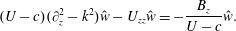 $$\begin{eqnarray}(U-c)(\unicode[STIX]{x2202}_{z}^{2}-k^{2}){\hat{w}}-U_{zz}{\hat{w}}=-\frac{B_{z}}{U-c}{\hat{w}}.\end{eqnarray}$$
 Here,  $k$ is the streamwise wavenumber of the perturbation, and $c=c_{r}+\text{i}c_{i}$ is the complex phase speed, so that the growth rate of a disturbance is given by $\unicode[STIX]{x1D70E}=kc_{i}$.
When kinematic viscosity  $\unicode[STIX]{x1D708}^{\ast }$ and diffusivity of the buoyancy distribution $\unicode[STIX]{x1D705}^{\ast }$ are taken into account, (2.1) becomes the more complicated pair of equations
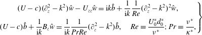 $$\begin{eqnarray}\left.\begin{array}{@{}c@{}}\displaystyle (U-c)(\unicode[STIX]{x2202}_{z}^{2}-k^{2}){\hat{w}}-U_{zz}{\hat{w}}=\text{i}k\hat{b}+\frac{1}{\text{i}k}\frac{1}{Re}(\unicode[STIX]{x2202}_{z}^{2}-k^{2})^{2}{\hat{w}},\\ \displaystyle (U-c)\hat{b}+\frac{1}{\text{i}k}B_{z}{\hat{w}}=\frac{1}{\text{i}k}\frac{1}{PrRe}(\unicode[STIX]{x2202}_{z}^{2}-k^{2})\hat{b},\quad Re\equiv \frac{U_{0}^{\ast }d_{0}^{\ast }}{\unicode[STIX]{x1D708}^{\ast }};Pr\equiv \frac{\unicode[STIX]{x1D708}^{\ast }}{\unicode[STIX]{x1D705}^{\ast }},\end{array}\right\}\end{eqnarray}$$
 where length scales and time scales have been non-dimensionalised using the half-depth  $d_{0}^{\ast }$ of the shear layer, and half the velocity difference $U_{0}^{\ast }$ across the shear layer, leading to a conventional definition of the Reynolds number, $Re$, and $Pr$ is the usual Prandtl number.
Following Hazel (Reference Hazel1972) and many subsequent authors, we consider the ‘Hazel’ model for the background velocity and buoyancy distributions
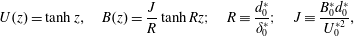 $$\begin{eqnarray}U(z)=\tanh z,\quad B(z)=\frac{J}{R}\tanh Rz;\quad R\equiv \frac{d_{0}^{\ast }}{\unicode[STIX]{x1D6FF}_{0}^{\ast }};\quad J\equiv \frac{B_{0}^{\ast }d_{0}^{\ast }}{U_{0}^{\ast 2}},\end{eqnarray}$$
 where  $\unicode[STIX]{x1D6FF}_{0}^{\ast }$ is the (dimensional) half-depth of the background buoyancy layer with half-difference $B_{0}^{\ast }$ and $J$ is the bulk Richardson number. This is an extension of the Holmboe model (Holmboe Reference Holmboe1960), which has $R=1$ and is attractive because the stability boundary can be found analytically (Miles Reference Miles1961). It is close to the self-similar error function profile expected for a diffusing stratified shear layer when $Pr=R^{2}$ (Smyth, Klaassen & Peltier Reference Smyth, Klaassen and Peltier1988). It is important to note that these profiles are not steady solutions of the viscous Boussinesq equations, but we make the ‘frozen flow’ approximation (Smyth & Carpenter Reference Smyth and Carpenter2019) which is valid when $\unicode[STIX]{x1D70E}\gg 1/Re$. This inequality is not always satisfied by the instabilities we find, as discussed in § 3.4.
The gradient Richardson number  $Ri_{g}$, defined as
 $$\begin{eqnarray}Ri_{g}(z)\equiv \frac{\text{d}B/\text{d}z}{(\text{d}U/\text{d}z)^{2}}=J\frac{\operatorname{sech}^{2}Rz}{\operatorname{sech}^{4}z},\end{eqnarray}$$
 for the Hazel model flow, which means (for this particular flow) that at the centreline,  $Ri_{g}(0)=J$. For $R\leqslant \sqrt{2}$, $J$ is the minimum of $Ri_{g}$, for $\sqrt{2}<R<2$, there are two minima of $Ri_{g}<J$ either side of local maximum $z=0$, and for $R\geqslant 2$, $Ri_{g}\rightarrow 0$ as $z\rightarrow \infty$ and $z=0$ is a global maximum (Alexakis Reference Alexakis2005). From the Miles–Howard theorem, we then deduce that inviscid HWI at arbitrarily large $J$ is only possible when $R\geqslant 2$. In fact, Alexakis (Reference Alexakis2007) showed that HWI only exists at all for $R\geqslant 2$, despite the possibility of instability at $J>1/4$ when $\sqrt{2}<R<2$.
The solution of (2.2) is performed using a MATLAB code from Smyth & Carpenter (Reference Smyth and Carpenter2019). The method is to construct a large matrix eigenvalue problem, using evenly spaced finite differences. This is a mature code, and additionally the existence of viscous Holmboe was confirmed in direct numerical simulation (DNS) of the Boussinesq equations at finite  $Re$ and $Pr=1$ (Parker et al. Reference Parker, Caulfield and Kerswell2019). The boundary conditions are that $\unicode[STIX]{x2202}{\hat{w}}/\unicode[STIX]{x2202}z=\unicode[STIX]{x2202}\hat{b}/\unicode[STIX]{x2202}z=0$, i.e. frictionless, insulating boundaries, at $z=\pm L_{z}$, although all of the instabilities we discuss here are centred around the shear layer, and changing the boundary conditions would not qualitatively affect the results. All linear stability results are found using $768$ finite difference points in the vertical direction, except for the $L_{z}=20$ case which used $1024$ points, and the figures are generated from a $48\times 48$ grid of calculated growth rates.
3 Linear stability analyses
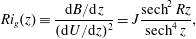
Figure 1 shows a typical example of the VHI. There is a clear distinction between those unstable modes with zero phase speed, which we identify as KHI, and the modes with non-zero phase speed, which we identify as VHI. Although the existence of unstable modes at  $R=1$ with non-zero phase speed was unknown before Parker et al. (Reference Parker, Caulfield and Kerswell2019), the diagram bears a striking resemblance to the classic stability diagrams for inviscid HWI for a piecewise linear profile with a density discontinuity (Holmboe Reference Holmboe1962, figure 7) and the Holmboe model with $R>2$ (Hazel Reference Hazel1972, figure 8). Crucially, above $J=0.25$ on this diagram, the gradient Richardson number of the flow is everywhere greater than one quarter, and so we expect stability as $Re\rightarrow \infty$. In the inviscid case, as $J$ is increased the dominant KHI mode and a subdominant KHI mode converge and bifurcate into the pair of HWI modes, with opposite phase speeds. In the viscous case, the regions of the two instabilities overlap slightly and there is no clean bifurcation from one to the other. The remainder of this section will explore how the structure of stability diagrams like figure 1 change as various parameters are varied.
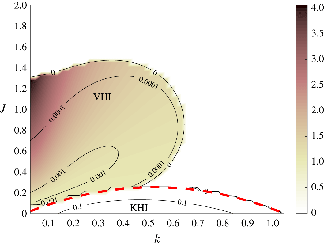
Figure 1. Stability diagram for the Hazel model flow profile as defined in (2.3) with  $R=1$, $Re=500$, $Pr=1$, with boundaries at $z=\pm L_{z}=\pm 15$. The contours show the growth rate of two-dimensional normal-mode perturbations of wavenumber $k$, at bulk Richardson number $J$. The colours show the phase speed. The lower region, up to $J=0.25$, is KHI with zero phase speed. The upper lobe is the VHI, with non-zero phase speed. The dashed line shows the analytic stability boundary $J=k(1-k)$ for an unbounded domain in the inviscid limit (Miles Reference Miles1961). In this, and all the stability diagrams in this paper, a waviness is apparent near stability boundaries. This is a common problem in such stability diagrams (Hogg & Ivey Reference Hogg and Ivey2003; Smyth & Winters Reference Smyth and Winters2003; Carpenter et al. Reference Carpenter, Balmforth and Lawrence2010, Reference Carpenter, Tedford, Heifetz and Lawrence2013), and is associated with interpolating near sharp changes of gradient in contour plots.
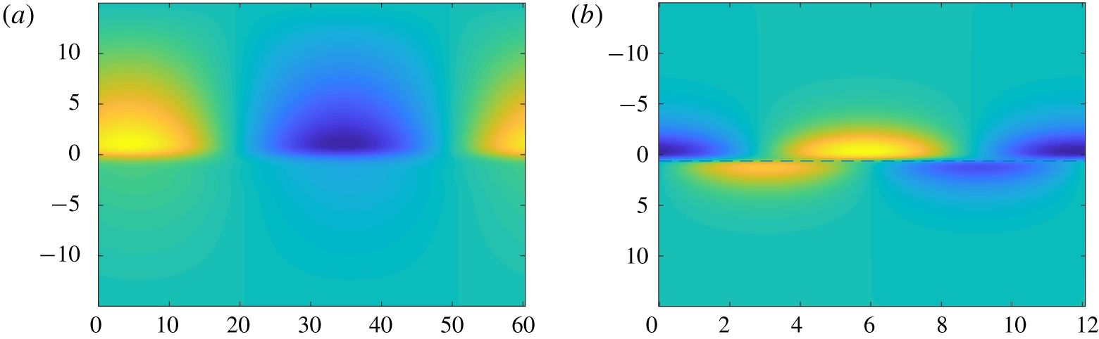
Figure 2. Vorticity field for the most unstable VHI mode for  $R=1$ ( $J=0.2128$, $k=0.1042$, a) and $R=3$ ( $J=0.8085$, $k=0.5208$, b). In the latter case, a critical layer exists at $z=0.63437$ and is marked with a dashed line.
Table 1. The various parameters used for the linear stability diagrams, as well as the maximum growth rate  $\unicode[STIX]{x1D70E}^{max}$ of VHI for each set of parameters, and the phase speed $c_{r}^{max}$, wavenumber $k^{max}$ and bulk Richardson number $J^{max}$ at which they occur.
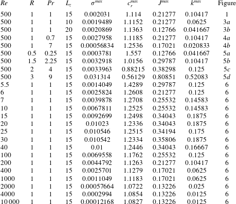
Figure 2 shows typical eigenmodes of the spanwise vorticity. With  $R=1$, i.e. a density interface as wide as the shear layer, no critical layer exists. With $R=3$, the eigenmode is virtually indistinguishable from the $Re\rightarrow \infty$ case, and a critical layer is present and clearly manifests itself within the spatial structure of the mode. Both of these modes have an equivalent mode associated with the complex conjugate eigenvalue, which is identical except for a reflection in the centreline. In the $R=1$ case, we also note that the growth rate is maximised at a much lower wavenumber.
Table 1 shows the full list of parameters for which stability diagrams were produced. For each diagram, we find the maximum growth rate for VHI, i.e. the maximum of  $\unicode[STIX]{x1D70E}$ such that the phase speed $c_{r}$ is non-zero, maximised over the discretised values of $k$ and $J$. Since the grids are relatively coarse, the values will not be the true maxima as no optimisation algorithm has been employed, but they give a strong indication of the trend.
3.1 Effects of domain height
The instabilities we study, KHI and HWI, were originally derived as solutions to the Taylor–Goldstein equation in an unbounded domain. There are several ways to approximate a domain of infinite height numerically, but we choose the simplest, which is to use a domain of sufficiently large, but finite, height. How large is sufficient is an important question, as a very large domain is computationally inefficient. Certainly as the height gets small compared with the wavelength of the instabilities we expect the results to change dramatically, and Hazel (Reference Hazel1972) noted how the diagrams always differ from the analytic, unbounded results at low wavenumbers. Figure 3 shows the same diagram as figure 1, but at a smaller (figure 3a) and a larger (figure 3b) domain height. Although the results are slightly different, qualitatively they are very similar, especially for  $L_{z}=20$, with $L_{z}=10$ showing more instability at low wavenumbers. The maximum growth rate of the VHI region is $\unicode[STIX]{x1D70E}=1.9489\times 10^{-3}$ for $L_{z}=10$ and $\unicode[STIX]{x1D70E}=2.0869\times 10^{-3}$ for $L_{z}=20$, compared with $\unicode[STIX]{x1D70E}=2.0310\times 10^{-3}$ for $L_{z}=15$, suggesting that $L_{z}=15$ is sufficient to capture the behaviour in which we are interested.
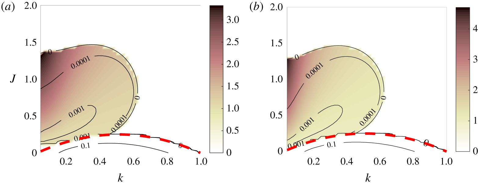
Figure 3. As for figure 1, but with  $L_{z}=10$ (a) and $L_{z}=20$ (b).
3.2 Effects of Prandtl number
Figure 4 shows the effect on the stability diagram of varying the Prandtl number. For  $Pr=0.7$ (characteristic of thermally stratified air), we find a maximum growth rate of $\unicode[STIX]{x1D70E}=2.7958\times 10^{-3}$, and for $Pr=7$ (a typical value for thermally stratified water) of $\unicode[STIX]{x1D70E}=5.6834\times 10^{-4}$, compared with $\unicode[STIX]{x1D70E}=2.0310\times 10^{-3}$ for $Pr=1$. Therefore, decreasing the diffusion of buoyancy seems to have a stabilising effect on VHI. In contrast, the KHI at the bottom of the figure is virtually unchanged as $Pr$ is varied by an order of magnitude, which reinforces the idea that KHI is produced by the shear alone. Jones (Reference Jones1977) found strong instability at very low $Pr$, but we believe this to be a different effect.
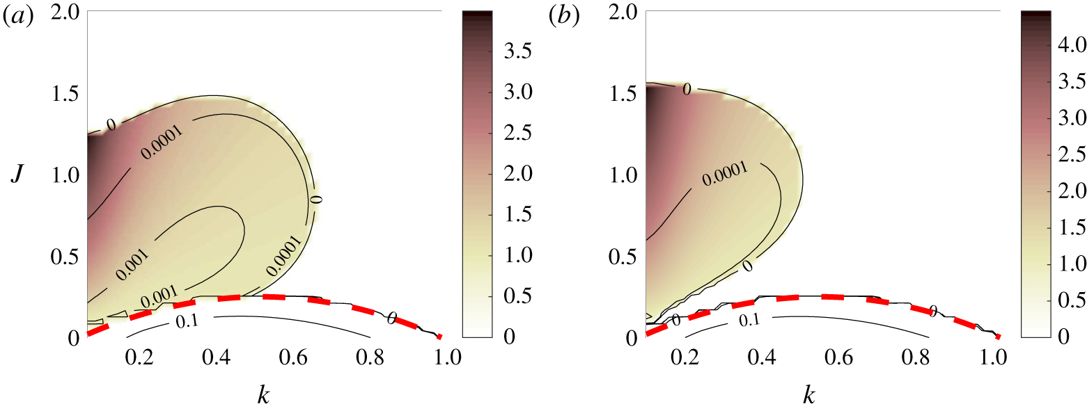
Figure 4. As for figure 1, but with  $Pr=0.7$ (a) and $Pr=7$ (b).
Henceforth, we give results using  $Pr=R^{2}$, as proposed by Smyth et al. (Reference Smyth, Klaassen and Peltier1988). Despite the fact that the instability seems to be destabilised when $Pr$ is reduced, it is also stabilised when $R$ is decreased, as we shall see.
3.3 Effects of  $R$
$R$

So far, the results we have presented have concentrated on  $R=1$, the original Holmboe model. However, in the inviscid limit, HWI exists only for $R>2$ (Alexakis Reference Alexakis2007). Figure 5 shows the stability diagram at $Re=500$ over a range of $R$, with $Pr=R^{2}$. All diagrams show a region of instability with non-zero phase speed, which we identify as VHI. In the case $R=3$, the diagram is very similar to the classical diagram of an inviscid fluid (Hazel Reference Hazel1972). The unstable region above the usual band, at low wavenumbers, has $c_{r}>1$, so there is no critical layer. As $R\rightarrow 2$ from above, the inviscid results suggest that the band should narrow to a line (Alexakis Reference Alexakis2005), but instead we see a significant region of instability. In the diagrams for $R=1.5$ and $R=2$, a second band of instability is observed above the first, with reduced phase speed, and we conjecture that this may be connected with the higher Holmboe modes. This has not been investigated further, as the growth rate here is vanishingly small.
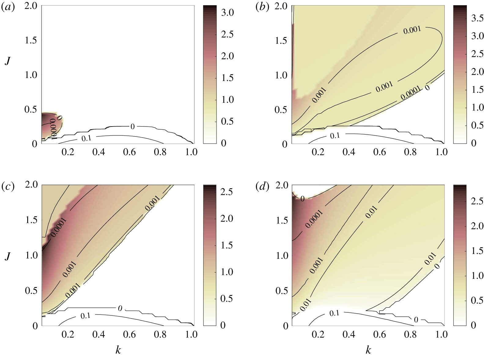
Figure 5. As for figure 1, but with (a)  $R=0.5$, $Pr=0.25$, (b) $R=1.5$, $Pr=2.25$, (c) $R=2$, $Pr=4$, (d) $R=3$, $Pr=9$. Only the last of these would exhibit HWI at $Re=\infty$.
In all cases, although it is not clear from the truncated diagrams, the instability is suppressed at large  $k$ by viscosity. This is in contrast to the inviscid limit, which has instability at arbitrarily large $k$ and $J$. It is only in this large $k$ limit that the wave interaction arguments can be made rigorous.
3.4 Effects of Reynolds number
The Miles–Howard theorem tells us that VHI at  $R=1$ must disappear for $J>1/4$, in the inviscid limit $Re\rightarrow \infty$. This leaves many possibilities: (i) the region of instability could retreat below $J=1/4$; (ii) the region could shrink; or (iii) the growth rates could vanish but the region remain a constant size. There may or may not be some finite $Re$ above which VHI does not exist. It is also important to ask at what value of $Re$ the growth of the instability is the fastest, or indeed the relative growth rate compared with the diffusion of the background profile.
The growth rate is maximised between  $Re=25$ and $Re=30$, with value $\unicode[STIX]{x1D70E}\approx 0.0105$. The relative growth rate $\unicode[STIX]{x1D70E}Re$, which is required to be large compared with unity for a physically relevant instability, was found to increase with $Re$ (at least until $Re=10\,000$), which is a curious result, since it means that despite the growth rate being maximised at a very low value of $Re$, in practice we are more likely to observe the instability at much higher $Re$.
$Re$.
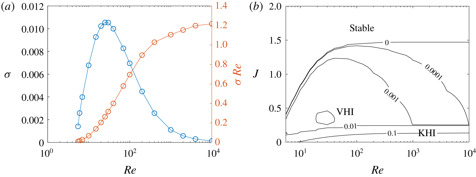
Figure 6. (a) The growth rate  $\unicode[STIX]{x1D70E}$ (left axis) and relative growth rate $\unicode[STIX]{x1D70E}Re$ (right axis), maximised over $k$ and $J$, for VHI at $R=1$, $Pr=1$, as $Re$ varies. (b) Growth rate against $J$ and $Re$, maximised over $k$, for $R=1$ and $Pr=1$. The band at the bottom of the figure is KHI, destabilised as $Re$ increases. The upper region with $J\gtrsim 1/4$ is VHI, clearly stabilised as $Re$ increases.
The critical Reynolds number  $Re_{c}$ for the viscous Holmboe instability at $R=1$, $Pr=1$, below which there is no instability except KHI, was found to be $Re=4.615$. At criticality, the instability appears at $J=0.25$ and $k=0.12$. This is in contrast with KHI, which at $J=0$ was found to have $Re_{c}=0$ (Betchov & Szewczyk Reference Betchov and Szewczyk1963). In that case, viscosity has a purely stabilising effect. Figure 6 shows how the growth rate varies with $Re$.
$Re$.
3.4.1 Asymptotic behaviour at high $Re$

The fact that some of the VHI do not have a critical layer ( $c_{r}^{max}>1$ in Table 1) suggests a regular perturbation analysis may be sufficient to capture the effect of high but finite $Re$. Defining a perturbation parameter $\unicode[STIX]{x1D716}:=1/Re\ll 1$, we may rewrite (2.2) as
 $$\begin{eqnarray}{\mathcal{L}}_{0}(c)\left(\begin{array}{@{}c@{}}{\hat{w}}\\ \hat{b}\end{array}\right)=\unicode[STIX]{x1D716}{\mathcal{L}}_{1}\left(\begin{array}{@{}c@{}}{\hat{w}}\\ \hat{b}\end{array}\right),\end{eqnarray}$$
where we have defined linear operators
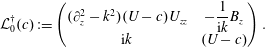
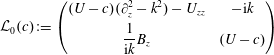 $$\begin{eqnarray}{\mathcal{L}}_{0}(c):=\left(\begin{array}{@{}cc@{}}(U-c)(\unicode[STIX]{x2202}_{z}^{2}-k^{2})-U_{zz} & -\text{i}k\\ \displaystyle \frac{1}{\text{i}k}B_{z} & (U-c)\end{array}\right)\end{eqnarray}$$
and
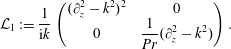 $$\begin{eqnarray}{\mathcal{L}}_{1}:=\frac{1}{\text{i}k}\left(\begin{array}{@{}cc@{}}(\unicode[STIX]{x2202}_{z}^{2}-k^{2})^{2} & 0\\ 0 & \displaystyle \frac{1}{Pr}(\unicode[STIX]{x2202}_{z}^{2}-k^{2})\end{array}\right).\end{eqnarray}$$
Adopting the expansions
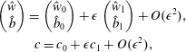 $$\begin{eqnarray}\displaystyle & \displaystyle \left(\begin{array}{@{}c@{}}{\hat{w}}\\ \hat{b}\end{array}\right)=\left(\begin{array}{@{}c@{}}{\hat{w}}_{0}\\ \hat{b}_{0}\end{array}\right)+\unicode[STIX]{x1D716}\left(\begin{array}{@{}c@{}}{\hat{w}}_{1}\\ \hat{b}_{1}\end{array}\right)+O(\unicode[STIX]{x1D716}^{2}), & \displaystyle \nonumber\\ \displaystyle & \displaystyle c=c_{0}+\unicode[STIX]{x1D716}c_{1}+O(\unicode[STIX]{x1D716}^{2}), & \displaystyle \nonumber\end{eqnarray}$$
 (keeping  $k$ fixed), then
 $$\begin{eqnarray}{\mathcal{L}}_{0}(c)={\mathcal{L}}_{0}(c_{0})+\unicode[STIX]{x1D716}c_{1}{\mathcal{L}}_{0}^{\prime }+O(\unicode[STIX]{x1D716}^{2}),\end{eqnarray}$$
where
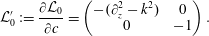 $$\begin{eqnarray}{\mathcal{L}}_{0}^{\prime }:=\frac{\unicode[STIX]{x2202}{\mathcal{L}}_{0}}{\unicode[STIX]{x2202}c}=\left(\begin{array}{@{}cc@{}}-(\unicode[STIX]{x2202}_{z}^{2}-k^{2}) & 0\\ 0 & -1\end{array}\right).\end{eqnarray}$$
Inserting these expansions into (3.1), we have
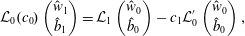
 $$\begin{eqnarray}{\mathcal{L}}_{0}(c_{0})\left(\begin{array}{@{}c@{}}{\hat{w}}_{0}\\ \hat{b}_{0}\end{array}\right)+\unicode[STIX]{x1D716}{\mathcal{L}}_{0}(c_{0})\left(\begin{array}{@{}c@{}}{\hat{w}}_{1}\\ \hat{b}_{1}\end{array}\right)+\unicode[STIX]{x1D716}c_{1}{\mathcal{L}}_{0}^{\prime }\left(\begin{array}{@{}c@{}}{\hat{w}}_{0}\\ \hat{b}_{0}\end{array}\right)=\unicode[STIX]{x1D716}{\mathcal{L}}_{1}\left(\begin{array}{@{}c@{}}{\hat{w}}_{0}\\ \hat{b}_{0}\end{array}\right)+O(\unicode[STIX]{x1D716}^{2}).\end{eqnarray}$$
At leading order, the inviscid Taylor–Goldstein equation is recovered,
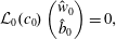 $$\begin{eqnarray}{\mathcal{L}}_{0}(c_{0})\left(\begin{array}{@{}c@{}}{\hat{w}}_{0}\\ \hat{b}_{0}\end{array}\right)=0,\end{eqnarray}$$
 which by the Miles–Howard theorem has only wavelike solutions  $c_{0}\in \mathbb{R}$ when $R=1$ and $J>1/4$. In this case, the diagonal elements of ${\mathcal{L}}_{0}(c)$ are real and the off-diagonal elements are purely imaginary, so that for a solution we must have $\arg \hat{b}_{0}=\arg {\hat{w}}_{0}\pm \unicode[STIX]{x03C0}/2$ in the absence of a critical layer. Without loss of generality, we may choose the phase so that ${\hat{w}}_{0}$ is real and $\hat{b}_{0}$ is purely imaginary.
With an inner product on the space of vectors
 $$\begin{eqnarray}\left\langle \left(\begin{array}{@{}c@{}}w_{1}\\ b_{1}\end{array}\right)\!,\left(\begin{array}{@{}c@{}}w_{2}\\ b_{2}\end{array}\right)\right\rangle :=\int _{L_{z}}^{L_{z}}(w_{1}^{\ast }w_{2}+b_{1}^{\ast }b_{2})\,\text{d}z,\end{eqnarray}$$
 we may define the adjoint operator  ${\mathcal{L}}_{0}^{\dagger }(c)$ to ${\mathcal{L}}_{0}(c)$ via
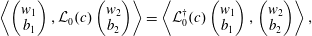 $$\begin{eqnarray}\left\langle \left(\begin{array}{@{}c@{}}w_{1}\\ b_{1}\end{array}\right),{\mathcal{L}}_{0}(c)\left(\begin{array}{@{}c@{}}w_{2}\\ b_{2}\end{array}\right)\right\rangle =\left\langle {\mathcal{L}}_{0}^{\dagger }(c)\left(\begin{array}{@{}c@{}}w_{1}\\ b_{1}\end{array}\right),\left(\begin{array}{@{}c@{}}w_{2}\\ b_{2}\end{array}\right)\right\rangle ,\end{eqnarray}$$
which gives
 $$\begin{eqnarray}{\mathcal{L}}_{0}^{\dagger }(c):=\left(\begin{array}{@{}cc@{}}(\unicode[STIX]{x2202}_{z}^{2}-k^{2})(U-c)U_{zz} & \displaystyle -\frac{1}{\text{i}k}B_{z}\\ \text{i}k & (U-c)\end{array}\right).\end{eqnarray}$$
The existence of a non-trivial solution to (3.7) implies a non-trivial solution to
 $$\begin{eqnarray}{\mathcal{L}}_{0}^{\dagger }(c_{0})\left(\begin{array}{@{}c@{}}{\hat{w}}_{0}^{\dagger }\\ \hat{b}_{0}^{\dagger }\end{array}\right)=0,\end{eqnarray}$$
 which is the adjoint eigenfunction. Again, we can choose  ${\hat{w}}_{0}^{\dagger }$ to be real and $\hat{b}_{0}^{\dagger }$ to be imaginary.
The  $O(\unicode[STIX]{x1D716})$ terms in (3.6) give
 $$\begin{eqnarray}{\mathcal{L}}_{0}(c_{0})\left(\begin{array}{@{}c@{}}{\hat{w}}_{1}\\ \hat{b}_{1}\end{array}\right)={\mathcal{L}}_{1}\left(\begin{array}{@{}c@{}}{\hat{w}}_{0}\\ \hat{b}_{0}\end{array}\right)-c_{1}{\mathcal{L}}_{0}^{\prime }\left(\begin{array}{@{}c@{}}{\hat{w}}_{0}\\ \hat{b}_{0}\end{array}\right),\end{eqnarray}$$
so taking the inner product with the adjoint eigenfunction, we have
 $$\begin{eqnarray}\left\langle \left(\begin{array}{@{}c@{}}{\hat{w}}_{0}^{\dagger }\\ \hat{b}_{0}^{\dagger }\end{array}\right),{\mathcal{L}}_{0}(c_{0})\left(\begin{array}{@{}c@{}}{\hat{w}}_{1}\\ \hat{b}_{1}\end{array}\right)\right\rangle =\left\langle \left(\begin{array}{@{}c@{}}{\hat{w}}_{0}^{\dagger }\\ \hat{b}_{0}^{\dagger }\end{array}\right),{\mathcal{L}}_{1}\left(\begin{array}{@{}c@{}}{\hat{w}}_{0}\\ \hat{b}_{0}\end{array}\right)\right\rangle -c_{1}\left\langle \left(\begin{array}{@{}c@{}}{\hat{w}}_{0}^{\dagger }\\ \hat{b}_{0}^{\dagger }\end{array}\right),{\mathcal{L}}_{0}^{\prime }\left(\begin{array}{@{}c@{}}{\hat{w}}_{0}\\ \hat{b}_{0}\end{array}\right)\right\rangle .\end{eqnarray}$$
The left-hand side of this equation is zero by construction, and so
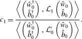 $$\begin{eqnarray}c_{1}=\frac{\displaystyle \left\langle \left(\begin{array}{@{}c@{}}{\hat{w}}_{0}^{\dagger }\\ \hat{b}_{0}^{\dagger }\end{array}\right),{\mathcal{L}}_{1}\left(\begin{array}{@{}c@{}}{\hat{w}}_{0}\\ \hat{b}_{0}\end{array}\right)\right\rangle }{\displaystyle \left\langle \left(\begin{array}{@{}c@{}}{\hat{w}}_{0}^{\dagger }\\ \hat{b}_{0}^{\dagger }\end{array}\right),{\mathcal{L}}_{0}^{\prime }\left(\begin{array}{@{}c@{}}{\hat{w}}_{0}\\ \hat{b}_{0}\end{array}\right)\right\rangle }.\end{eqnarray}$$
 Observe from (3.3) and (3.5) that  ${\mathcal{L}}_{1}$ and ${\mathcal{L}}_{0}^{\prime }$ are purely imaginary and real respectively. By our choice of phase it is clear that the numerator is therefore imaginary and the denominator real, so $c_{1}$ is purely imaginary. It can be similarly shown that $c_{2}$ is real so the next contribution to the growth rate is at $O(1/Re^{3})$. We further observe that both ${\mathcal{L}}_{1}$ and $c_{1}{\mathcal{L}}_{0}^{\prime }$ are purely imaginary, so from (3.12) we deduce that ${\hat{w}}_{1}$ and $\hat{b}_{1}$ are purely imaginary and real respectively, the opposite situation to ${\hat{w}}_{0}$ and $\hat{b}_{0}$.
We compute  $c_{1}$, and thus the growth rate of the instability as $Re$ becomes large $\unicode[STIX]{x1D70E}=-\text{i}kc_{1}/Re+O(1/Re^{3})$, using (3.14) as follows. First, we make an initial guess of $c_{0}$ from the real part of $c$ from a numerical linear stability analysis at $Re=10\,000$. Secondly, we use this approximate $c_{0}$ in the inverse iteration eigenvalue algorithm to solve both (3.7) and (3.11). Finally, we directly evaluate (3.14) using a trapezoidal quadrature rule for the inner products.
The results for two sample parameter values are shown in figure 7(a). Figure 7(b) shows calculated zeroth- and first-order modes. We thus see that the viscous Holmboe modes are a destabilisation of a stable, propagating mode in the inviscid limit. Viscosity acts to break the exact  $\unicode[STIX]{x03C0}/2$ phase difference between the vertical velocity and the buoyancy modes. The fact that VHI varies smoothly between modes with and without critical layers, in particular in figure 5(c), suggests this regular perturbation analysis will extend to the case where a critical layer exists, and that the critical layer is not important to the dynamics.
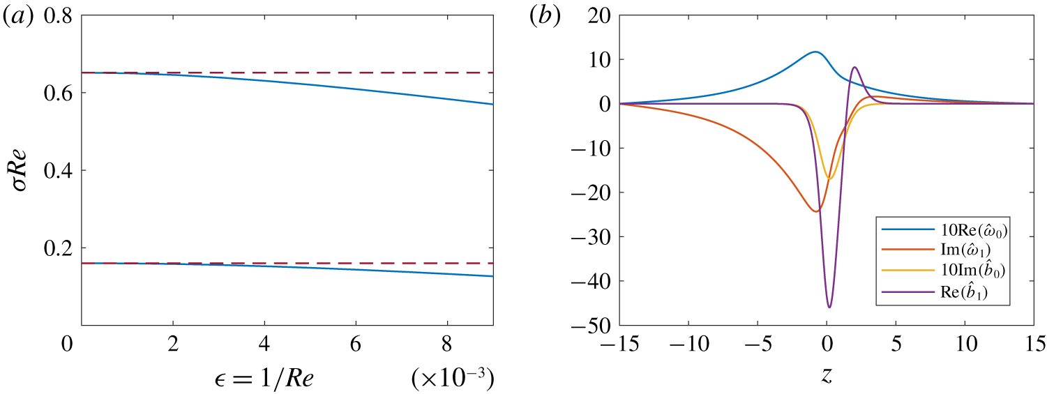
Figure 7. (a) Asymptotic (dashed) and numerical (solid) values of growth rate for VHI at  $J=1$, $k=0.5$ (lower) and $J=0.5$, $k=0.25$ (upper). (b) Modes for the $J=0.5$, $k=0.25$ case. The zeroth order modes have been scaled for clarity. In both panels, $R=1$, $Pr=1$ and $L_{z}=15$, corresponding to figure 1.
4 Nonlinear evolution
Smyth & Peltier (Reference Smyth and Peltier1990) showed that at low Reynolds numbers, the linear evolution of HWI is insufficiently fast to overcome the diffusion of the background flow. This leads to the possibility that VHI, for which the growth rates are always small, never physically manifests when the background flow is allowed to diffuse. We consider the nonlinear evolution, which allows us to see whether the viscous Holmboe instability develops the classic counter-propagating vortices of HWI. We use the same DNS code as Parker et al. (Reference Parker, Caulfield and Kerswell2019) to solve the full Boussinesq equations, which is pseudospectral in the streamwise direction and utilises finite differences in the vertical. In the present case, the background flow is allowed to diffuse.
Here we present the results of two direct numerical simulations (restricted to two dimensions) with  $R=1.5$, a case for which no HWI is predicted in the inviscid limit. We take $Re=4000$, a compromise between maximising the relative growth rate (see § 3.4) and minimising the spatial resolution. We chose a domain width of $L_{x}=20$, which permits multiple unstable modes. Figure 8 shows the results of a calculation with $J=0.1$, for which we expect a Kelvin–Helmholtz instability to develop to finite amplitude. A linear stability analysis predicts exponential growth rates of $\unicode[STIX]{x1D70E}=0.1244$ and $\unicode[STIX]{x1D70E}=0.0981$ for mode 1 and mode 2 disturbances ( $k=\unicode[STIX]{x03C0}/10$ and $k=\unicode[STIX]{x03C0}/5$) respectively, in both cases with zero phase speed. We use a relatively large initial perturbation of random noise in low wavenumber Fourier and Hermite modes, which, along with the comparable growth rates for the two unstable modes, leads to an incoherent, but nevertheless recognisable, Kelvin–Helmholtz billow. At the large $Re$ studied, this rapidly breaks down into turbulence, and significant mixing is achieved, although it is important to remember that this DNS is restricted to two dimensions, and so the specific characteristics of the mixing are likely to be unphysical.
Figure 9 shows the same calculation with  $J=0.67$, which maximises the growth rate for VHI at this wavenumber. Again, both modes 1 and 2 are unstable, with growth rates $\unicode[STIX]{x1D70E}=4.1121\times 10^{-4}$ and $\unicode[STIX]{x1D70E}=1.7012\times 10^{-4}$ respectively, and phase velocities $c_{r}=\pm 1.0211$ and $c_{r}=\pm 1.0056$. Since the phase speeds are greater than $1$, no critical layer exists for these instabilities. In this case, the relative growth rate clearly does not satisfy
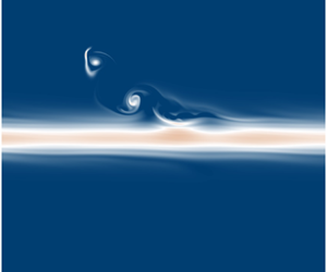
  $\unicode[STIX]{x1D70E}Re\gg 1$, so we require a large initial perturbation to trigger significant instability. The strong asymmetry of this random perturbation means that a Holmboe ‘wave’ is apparent only on one side of the interface. Despite the lack of a critical layer, a ‘cusped wave’ very reminiscent of classic HWI (Alexakis Reference Alexakis2009; Salehipour et al. Reference Salehipour, Caulfield and Peltier2016) is apparent, and grows large enough for a clear vortex to be apparent. This vortex is responsible for some mixing, which can be observed when comparing the long time vorticity distribution above the interface, where the vortex exists, to below, where no strong VHI was triggered. However, this mixing is relatively weak compared with the diffusion of the background profile. It is difficult to define a speed precisely for the nonlinear wave, but it appears to be close to $1$. Both the background flow velocity at the level of the vortices and the phase velocity of the linear instability are also approximately equal to $1$. Animations of both evolving flows are available as supplementary materials.
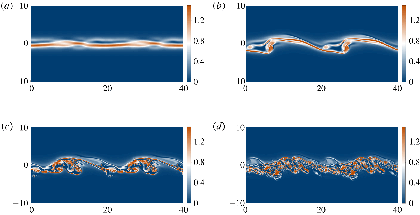
Figure 8. The total vorticity field of a two-dimensional nonlinear simulation of the Boussinesq equations at  $Re=4000$, $Pr=2.25$, $L_{x}=20$, $L_{z}=10$ and $J=0.1$. The initial state is a background field with $R=1.5$, plus a perturbation of random noise in the first sixth of the horizontal Fourier modes, and the first five Hermite polynomials in the vertical. Two domain widths are shown horizontally: (a) $t=0$, showing the random initial conditions; (b) $t=20$, showing the Kelvin–Helmholtz billow that has begun to develop; (c) $t=40$, showing that the billow has saturated and is starting to break down; (d) $t=60$, showing that the KHI has led to (two-dimensional) turbulence. An animation of the evolving flow is available as supplementary movies 1 and 2 at https://doi.org/10.1017/jfm.2020.340.
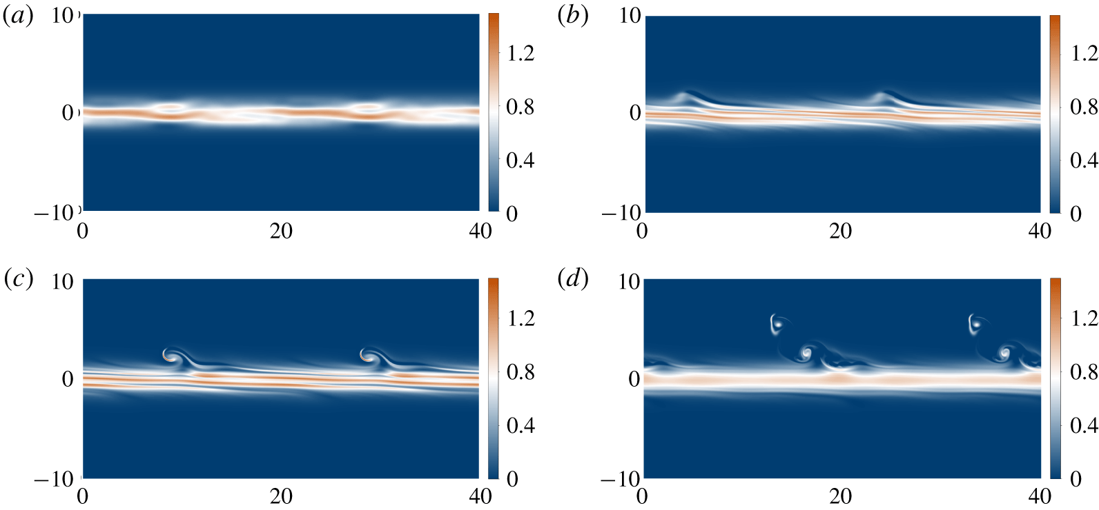
Figure 9. As for figure 8, but with  $J=0.4355$: (a) $t=0$, showing the random initial conditions; (b) $t=20$, showing that a ‘cusped wave’ is apparent, characteristic of HWI at finite amplitude; (c) $t=35$, showing that a leftwards-propagating vortex is now visible above the shear layer; (d) $t=110$, showing that the vortex has weakened as the mixing layer diffuses away. An animation of the evolving flow is available as supplementary movies 3 and 4.
5 Discussion and conclusions
In this paper, we have described a new, inherently viscous instability and have demonstrated that it shares many of the characteristic features of the classic, inviscid Holmboe wave instability, namely manifesting as a propagating vortex on either side of the mixing layer and appearing to be caused by the interaction of internal gravity waves on a shear interface. Since it exists in regions of parameter space where no instability is predicted in the inviscid limit, we term it the viscous Holmboe instability, or VHI. The instability we have described is distinct from the ‘viscous Holmboe wave instability’ found by Eaves & Caulfield (Reference Eaves and Caulfield2017) in plane Couette flow, which required non-slip and non-penetration effects in the presence of a rigid boundary, whereas we have shown that boundaries only weakly affect the instability, and the VHI discussed here is truly an instability of a stratified shear layer. Despite the similarities to inviscid HWI, it has significant differences from the classical case: it exists when the density interface is not sharp compared with the shear layer; it can have a phase speed greater than the maximum fluid velocity; and it is destabilised by viscosity. When there is no critical layer, a simple perturbation analysis shows that the VHI arises by viscosity disrupting the perfectly out-of-phase velocity and buoyancy components of the neutrally stable inviscid limit. Our work has made the ‘frozen flow’ approximation that requires  $\unicode[STIX]{x1D70E}$ to be large compared with $1/Re$ for the instability to grow quickly compared with the diffusion of the background profile, but we did not find this to be the case. Indeed, our perturbation analysis shows that $\unicode[STIX]{x1D70E}\sim 1/Re$ as $Re\rightarrow \infty$. Numerically, we find that $\unicode[STIX]{x1D70E}$ is small compared with $1/Re$ when $Re\lesssim 10^{2}$, despite the fact that $\unicode[STIX]{x1D70E}$ is maximised for $Re\approx 25$ and only just rises above $1/Re$ for $Re\gtrsim 10^{3}$. This leads to the curious situation that although this is an instability which requires viscosity to exist, the effect of the instability relative to the diffusion of the background flow appears to be greater as $Re$ is increased.
This work is a study of how viscosity affects the Holmboe wave instability as certain parameters are varied. There are many possible extensions which have been examined for (classic) HWI, including considering the effects of compressibility (Witzke, Silvers & Favier Reference Witzke, Silvers and Favier2015), surface tension (Pouliquen, Chomaz & Huerre Reference Pouliquen, Chomaz and Huerre1994), and relaxing the Boussinesq approximation (Umurhan & Heifetz Reference Umurhan and Heifetz2007; Churilov Reference Churilov2019). We briefly investigated the possibility that the higher Holmboe modes described by Alexakis (Reference Alexakis2005, Reference Alexakis2007, Reference Alexakis2009) are also destabilised by viscosity at low  $R$, and did indeed find a further band of instability with very small growth rates. Our work has been entirely restricted to two dimensions. Although this is a common assumption when studying linear instabilities of shear flows, there is no physical basis for this, and indeed we would fully expect to see the fastest growing mode being three-dimensional in some regions of parameter space, based on the results of Smyth & Peltier (Reference Smyth and Peltier1990). A third dimension would also significantly affect the nonlinear evolution of the instability at high $Re$.
$Re$.
Despite the lack of a sharp density interface relative to the shear layer for the parameters for which we have found instability, we would certainly still expect internal gravity waves to be present on the interface. There is no reason we are aware of, a priori, to think that these could not resonate with the vorticity waves to cause instability. The wave-resonance descriptions of stratified shear instabilities have been mainly qualitative, except in the cases of piecewise constant density and vorticity profiles, which would be physically inconsistent at finite viscosity. Recent attempts to analyse the components of resonances (Carpenter et al. Reference Carpenter, Balmforth and Lawrence2010; Eaves & Balmforth Reference Eaves and Balmforth2019) and to understand better the dynamics of the resonant system (Heifetz & Guha Reference Heifetz and Guha2018, Reference Heifetz and Guha2019) have relied on analysis which requires perturbations to be inviscid, and these certainly would not apply in the low  $Re$ regimes we have described. Though the theory of wave resonance has given useful insight in many situations, it is clearly not the full picture. One major outstanding question is how the Miles–Howard criterion may relate to the wave resonance picture. Baines & Mitsudera (Reference Baines and Mitsudera1994) give an argument from critical layer theory, although the authors themselves admit that this gives neither a necessary nor sufficient criterion for stability.
Most of the unstable regions of the viscous Holmboe instability for  $R\leqslant 2$ have $|c_{r}|>1$, so there is no critical layer. Therefore, Lindzen’s wave over-reflection hypothesis for the mechanism of stratified shear instabilities, as well as other interpretations based on the existence of a critical layer, such as the wave–particle interaction described by Churilov (Reference Churilov2019), cannot apply. This is in contrast with the viscous instability described by Miller & Lindzen (Reference Miller and Lindzen1988), in which the viscosity was thought to enable over-reflection at the critical layer. As discussed by Smyth & Peltier (Reference Smyth and Peltier1989), it could be possible that the instability is associated with over-reflection of a wave with a different phase speed, which therefore could itself have a critical layer, but this makes an intuitive explanation much harder. Since the wave over-reflection theory is not a predictive explanation of the instability in this case, it does not seem useful here, although it has certainly proven important in many other circumstances.
Under carefully controlled parameters, we have been able to show significant nonlinear growth of the viscous Holmboe instability at  $R=1.5$ and $Re=4000$, from initial noise, leading to secondary instabilities and transition to disorder. This primary instability has no critical layer. Nevertheless, most of the regions of instability we have studied, with $R<2$, have much lower growth rates. We conclude that the viscous Holmboe instability is unlikely to be particularly significant in physical processes. In addition to this, for typical values of Prandtl number in the atmosphere ( $Pr\approx 0.7$) we see very small growth rates and for typical values of $Pr\approx 7$ in the oceans, we see the full classical HWI, since in this case $R$ is usually large.
Despite these caveats, we have demonstrated the definite existence of an instability which bears a striking resemblance to HWI, but violates many of the supposed prerequisite conditions. We therefore suggest that any instability in a stratified shear layer be considered Holmboe instability if it manifests as propagating vortices on either side of the shear layer, regardless of the relative width of the density interface, the presence of critical layers or the minimum value of the gradient Richardson number.
Acknowledgements
We thank an anonymous referee for suggesting the perturbation analysis included. The linear stability analysis code was written by W. D. Smyth and we thank him for support with this. J.P.P. is supported by an EPSRC DTA studentship.
Declaration of interests
The authors report no conflict of interest.
Supplementary movies
Supplementary movies are available at https://doi.org/10.1017/jfm.2020.340.


 Open access