


1. Introduction
Turbulence is a chaotic, spatio-temporal multi-scale nonlinear phenomenon. Thus, it generally requires huge costs to accurately measure or simulate with sufficiently high resolution. In particular, direct numerical simulation has been actively used in the study of turbulence. However, securing the computational resources needed to resolve even the smallest-scale motions of turbulence is progressively challenging with high Reynolds numbers. To help resolve this problem, a neural network (NN), which has the ability to approximate arbitrary nonlinear functions (Hornik, Stinchcombe & White Reference Hornik, Stinchcombe and White1989), as well as linear-theory based methods such as proper orthogonal decomposition (Berkooz, Holmes & Lumley Reference Berkooz, Holmes and Lumley1993), linear stochastic estimation and Kalman filter have been studied. Indeed, there have been attempts to apply neural networks to represent turbulence (Lee et al. Reference Lee, Kim, Babcock and Goodman1997; Milano & Koumoutsakos Reference Milano and Koumoutsakos2002). However, those applications were based on shallow learning and, thus, were restricted to the extraction of simple correlations between turbulence quantities at two close locations in a near-wall flow. In recent years, deep neural networks (DNN) have been extended to various fields of turbulence research, owing to the development of data-driven learning algorithms (e.g. deep learning LeCun, Bengio & Hinton Reference LeCun, Bengio and Hinton2015), computational equipment (e.g. graphical process units), big data (e.g. Johns–Hopkins Turbulence Database (JHTDB) Perlman et al. Reference Perlman, Burns, Li and Meneveau2007) and open-source code (e.g. TensorFlow Abadi et al. Reference Abadi2015).
Various deep-learning applications have recently been developed for broad areas of turbulence research (Kutz Reference Kutz2017; Brenner, Eldredge & Freund Reference Brenner, Eldredge and Freund2019; Duraisamy, Iaccarino & Xiao Reference Duraisamy, Iaccarino and Xiao2019; Brunton, Noack & Koumoutsakos Reference Brunton, Noack and Koumoutsakos2020; Fukami, Fukagata & Taira Reference Fukami, Fukagata and Taira2020a; Pandey, Schumacher & Sreenivasan Reference Pandey, Schumacher and Sreenivasan2020). Ling, Kurzawski & Templeton (Reference Ling, Kurzawski and Templeton2016) proposed a tensor-based NN by embedding the Galilean invariance of a Reynolds-averaged Navier–Stokes (RANS) model, showing a greater performance improvement than linear and nonlinear eddy viscosity models. Parish & Duraisamy (Reference Parish and Duraisamy2016), Wang, Wu & Xiao (Reference Wang, Wu and Xiao2017), and other researchers have actively engaged in improving RANS models (e.g. Kutz Reference Kutz2017; Duraisamy et al. Reference Duraisamy, Iaccarino and Xiao2019). On the other hand, Gamahara & Hattori (Reference Gamahara and Hattori2017) proposed a large-eddy simulation (LES)-closure model based on DNN for wall-bounded turbulence. It was then extended to other flows, such as two-dimensional (2-D) turbulence (Maulik et al. Reference Maulik, San, Rasheed and Vedula2019) and homogeneous isotropic turbulence (Beck, Flad & Munz Reference Beck, Flad and Munz2019; Xie et al. Reference Xie, Wang, Li and Ma2019). Additionally, the prediction of the temporal evolution of turbulent flows has been actively pursued. As a fundamental example, Lee & You (Reference Lee and You2019) studied the historical prediction of flow around a cylinder using generative adversarial networks. Srinivasan et al. (Reference Srinivasan, Guastoni, Azizpour, Schlatter and Vinuesa2019) predicted the temporal behaviour of simplified shear turbulence expressed as solutions of nine ordinary differential equations using a recurrent NN (RNN). Kim & Lee (Reference Kim and Lee2020a) proposed a high-resolution inflow turbulence generator at various Reynolds numbers, combining a generative adversarial network (GAN) and an RNN. As another noticeable attempt to apply machine learning to fluid dynamics, Raissi, Yazdani & Karniadakis (Reference Raissi, Yazdani and Karniadakis2020) reconstructed velocity and pressure fields from only visualizable concentration data based on a physics-informed NN framework. Recently, deep-reinforcement learning has been applied to fluid dynamics, such as observations of how swimmers efficiently use energy (Verma, Novati & Koumoutsakos Reference Verma, Novati and Koumoutsakos2018) and the development of a new flow-control scheme (Rabault et al. Reference Rabault, Kuchta, Jensen, Réglade and Cerardi2019).
Apart from the above studies, the super-resolution reconstruction of turbulent flows has recently emerged as an interesting topic. This capability would help researchers overcome environments in which only partial or low-resolution spatio-temporal data are available, owing to the limitations of measurement equipment or computational resources. Particularly, if direct numerical simulation (DNS)-quality data could be reconstructed from data obtained via LES, it would be very helpful for subgrid scale modelling. Maulik & San (Reference Maulik and San2017) proposed a shallow NN model that could recover a turbulent flow field from a filtered or noise-added one. Fukami, Fukagata & Taira (Reference Fukami, Fukagata and Taira2019a, Reference Fukami, Fukagata and Taira2020b) and Liu et al. (Reference Liu, Tang, Huang and Lu2020) reconstructed a flow field from a low-resolution filtered field using a convolutional NN (CNN). The method shows significant potential. The CNNs were trained to reduce the mean-squared error (MSE) between the predicted and true values of target quantities. However, small-scale structures were not represented well, and non-physical features were observed when the resolution ratio between the target and input fields was large. Deng et al. (Reference Deng, He, Liu and Kim2019) considered flow data around a cylinder measured using particle image velocimetry (PIV) in a learning network using a GAN in which the small-scale structures were better expressed than when only MSE was used. Similarly, Xie et al. (Reference Xie, Franz, Chu and Thuerey2018) and Werhahn et al. (Reference Werhahn, Xie, Chu and Thuerey2019) applied GANs on super-resolution smoke data. In all these prior studies, researchers used a supervised deep-learning model, which required labelled low- and high-resolution data for training. Therefore, paired data were artificially generated by filtering or averaging so that supervised learning could be made possible. In a more practical environment, however, only unpaired data are available (e.g. LES data in the absence of corresponding DNS data or measured data using PIV with limited resolution). For more practical and wider applications, a more generalized model that can be applied, even when paired data are not available, is needed. Kim & Lee (Reference Kim and Lee2020a) recently showed that unsupervised learning networks could generate turbulent flow fields for inflow boundary conditions from random initial seeds. This indeed demonstrates that a DNN can learn and reflect hidden similarities in unpaired turbulence. Based on this evidence, we presume that super-resolution reconstruction of unpaired turbulence is now possible by learning the similarities among the unpaired data. Such an extension would enable outcomes previously thought impossible. For example, the simultaneous learning of LES and DNS data becomes possible, and, thus, high-resolution turbulence fields with DNS quality can be reconstructed from LES fields. This can be useful for the development of subgrid-scale models through the production of paired data. Another example is the denoising and resolution enhancement of real-world data such as PIV measurements. This can be accomplished by learning noise-added experimental data and high-fidelity (experimental or simulation) data simultaneously. These are only a few examples of the new possibilities.
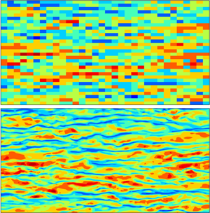
In this paper we propose an unsupervised deep-learning model that can be used, even in the absence of labelled turbulent data. For a super-resolution reconstruction using unpaired data, we apply a cycle-consistent GAN (CycleGAN) (Zhu et al. Reference Zhu, Park, Isola and Efros2017) to various turbulent flows as an unsupervised learning model. The detailed methodology is presented in § 2. For comparison, we use bicubic interpolation and supervised learning models (i.e. CNN and conditional GAN (cGAN)). The models are applied to three examples, as shown in figure 1. First, with homogeneous isotropic turbulence, a reconstruction of the DNS flow field from a top-hat-filtered (i.e. low-resolution) one is considered in § 3.1. Next, in § 3.2 we cover the reconstruction of full DNS data from a partially measured (i.e. low-resolution) one in wall-bounded turbulence. In §§ 3.1 and 3.2 we train our CycleGAN model using unpaired datasets with supervised learning models using paired ones. Finally, in § 3.3 DNS-quality reconstruction from LES is addressed using independently obtained LES and DNS data of wall-bounded turbulence. In this case, only the unsupervised learning model is applicable. We conclude our study with a discussion in § 4.

Figure 1. Illustration of present work. The proposed CycleGAN is an unsupervised learning model for the super-resolution reconstruction of turbulence. For comparison, CNN and cGAN are used as supervised learning models. In this study, three examples including filtered homogeneous and isotropic turbulence, partially measured wall-bounded turbulence, and large-eddy simulation (LES), are considered.
2. Methodology
In this study we apply CycleGAN to an unsupervised learning task. A typical GAN model consists of two networks: a generator network ( $G$) and a discriminator network ( $D$) (Goodfellow et al. Reference Goodfellow, Pouget-Abadie, Mirza, Xu, Warde-Farley, Ozair, Courville and Bengio2014). In the field of image generation, $G$ generates a fake image similar to the real one by applying convolution and upsampling to random noise $z$;
$z$;  $D$ distinguishes between the fake image and the real one and returns a probability value between 0 and 1 by applying convolution and downsampling. The final goal is to obtain $G$, which can generate fake images that are difficult to distinguish from real ones. This process is similar to a min–max two-player game for the value function, $V(D,G)$,
 \begin{equation} \min_{G} \max_{D} V(D,G) = \mathbb{E}_{x\sim P_{X}}[\log D(x)] + \mathbb{E}_{z\sim P_{Z}}[\log(1-D(G(z)))], \end{equation}
where  $X$ is a real image set, and $x\sim P_{X}$ means that $x$ is sampled from the real image distribution. Here $z$ is a random noise vector of latent space used as the input to the generator. Network $G$ is expected to generate a fake image similar to the real one. Thus, trainable parameters in $G$ are trained in the direction of $D(G(z))$, having a value close to 1. On the other hand, those in $D$ are trained in the direction of $D(x)$, returning a value close to 1. The term $D(G(z))$ returns a value close to 0. Thus, even a slight difference between the real image and the generated one can be distinguished. In other words, the $G$ parameters are adjusted in a direction that minimizes $V(D,G)$, and $D$ parameters are adjusted in a direction that maximizes $V(D,G)$. From this competitive learning, we can expect to obtain a generator, $G$, capable of providing a new image having a distribution similar to a real one. In the present work, GAN is applied to super-resolution reconstruction in the frame of finding an input–output mapping function, and, instead of random noise, low-resolution image data are used as the input of $G$, as illustrated in figure 2.

Figure 2. The GAN architecture consists of two networks, the generator (G) and the discriminator (D). Here  $G$ learns to reconstruct the high-resolution flow field ( $\tilde {Y}^{HR}$) from the low-resolution field ( ${X}^{LR}$), while $D$ learns to distinguish $\tilde {Y}^{HR}$ from the target field ( $Y^{HR}$).
For an unsupervised learning model of unpaired turbulence, we adopt CycleGAN (Zhu et al. Reference Zhu, Park, Isola and Efros2017) to find a mapping function between unpaired data,  $X$ and $Y$. We aim to obtain a model that performs super-resolution reconstruction when the low- and high-resolution flow fields are not matched. Here $X$ and $Y$ are low- and high-resolution datasets, respectively. CycleGAN consists of two generator networks, $(G, F)$, and two discriminator networks, $(D_Y, D_X)$, as shown in figure 3(a,b). Generators $G$ and $F$ are networks mapping $X \longrightarrow Y$ and $Y \longrightarrow X$, respectively. Discriminators $D_Y$ and $D_X$ distinguish between a fake image from generators and a real image, returning a probability value. Here $D_Y$ distinguishes between $G(x)$ generated by $G$ and $y$ from $Y$, whereas $D_X$ distinguishes between $F(y)$ generated by $F$ and $x$ from $X$. The objective function of CycleGAN consists of the GAN and cycle-consistency losses. The GAN loss helps the generators find the distribution of the target image. The cycle-consistency loss connects two generators, $(G,F)$, and reflects the dependency of input on them. First, the GAN loss function is used as
 \begin{gather} \mathcal{L}_{GAN}(G,D_Y) = \mathbb{E}_{y\sim P_{Y}}[\log D_Y(y)] + \mathbb{E}_{x\sim P_{X}}[\log(1-D_Y(G(x)))], \end{gather}
 \begin{gather}\mathcal{L}_{GAN}(F,D_X) = \mathbb{E}_{x\sim P_{X}}[\log D_X(x)] + \mathbb{E}_{y\sim P_{Y}}[\log(1-D_X(F(y)))], \end{gather}
where  $x$ and $y$ are the images sampled from $X$ and $Y$ datasets, respectively. Here $G$ is trained in a direction to minimize $\mathcal {L}_{GAN}(G,D_Y)$, and discriminator $D_Y$ is trained in a direction to maximize $\mathcal {L}_{GAN}(G,D_Y)$; $F$ and $D_X$ in (2.3) are trained in the same way.

Figure 3. CycleGAN architecture consisting of (a) forward GAN and (b) backward GAN. Here  $G$ and $F$ are generators, and $D_Y$ and $D_X$ are discriminators. (c) Forward cycle-consistency loss: $x\rightarrow G(x)\rightarrow F(G(x)) \approx x$, and backward cycle-consistency loss: $y\rightarrow F(y)\rightarrow G(F(y)) \approx y$.
In principle, the properly trained generators,  $G$ and $F$, can provide data having a similar distributions as the target data, $Y$ and $X$. However, the above loss cannot guarantee that the generated image will be properly dependent upon the input image. In other words, the high-resolution image, $G(x)$, from the low-resolution one, $x$, could have the characteristics of target datasets, $Y$, and the reconstructed image, $G(x)$, might not have a large-scale similarity to the low-resolution one, $x$. Therefore, a cycle-consistent loss that reduces the space of the mapping function with $G$ and $F$ is additionally used (see figure 3c). The cycle-consistent loss helps to ensure the dependency of the generated data on the input. This loss function consists of two terms for domains $X$ and $Y$. In the left panel of figure 3(c), the forward cycle-consistency loss reduces the space of image $x$ and $F(G(x))$ in domain $X$. It makes $G(x)$ dependent upon $x$ (
$x$ ( $x \rightarrow G(x) \rightarrow F(G(x)) \approx x$). Similarly, in the right panel of figure 3(c), the backward cycle-consistency loss reduces the space of image $y$ and $G(F(y))$ in domain $Y$ and makes $F(y)$ dependent upon $y$ (
$y$ ( $y \rightarrow F(y) \rightarrow G(F(y)) \approx y$). The cycle-consistency losses can be expressed as
 \begin{equation} \mathcal{L}_{cycle}(G,F) =\mathbb{E}_{x\sim P_{X}}[\parallel F(G(x)) - x\parallel^2_2] + \mathbb{E}_{y\sim P_{Y}}[\parallel G(F(y)) - y\parallel^2_2], \end{equation}
where the first term on the right-hand side is the forward cycle-consistency loss, and the second term is the backward cycle-consistency loss. Here  $\parallel \parallel ^2_2$ denotes mean-squared error, which is normalized by vector size. The MSE between $F(G(x))$ and $x$ and that between $G(F(y))$ and $y$ are used. The cycle-consistency loss provides a decisive effect on learning the unpaired data. The final objective function used in this study is
 \begin{equation} \mathcal{L}(G,F,D_Y,D_X) = \mathcal{L}_{GAN}(G,D_Y) + \mathcal{L}_{GAN}(F,D_X) + \lambda \mathcal{L}_{cycle}(G,F), \end{equation}
where  $\lambda$ is a weight factor and is fixed at $10$. Generators $G$ and $F$ are trained in the direction of minimizing $\mathcal {L}(G,F,D_Y,D_X)$, whereas discriminators $D_Y$ and $D_X$ are trained in the direction of maximizing $\mathcal {L}(G,F,D_Y,D_X)$. Learning with the above GAN loss often diverges, because the discriminator easily distinguishes between the generated image and the target one before parameters in the generator are sufficiently trained. Additionally, there is a well-known problem (i.e. mode collapse) in which the generation distribution is restricted to a small domain, although training does not diverge. To solve this problem, we change the above GAN loss to a Wasserstein GAN (WGAN) having a gradient penalty (GP) loss (Gulrajani et al. Reference Gulrajani, Ahmed, Arjovsky, Dumoulin and Courville2017). With the WGAN-GP loss, the GP term is added, and the probabilistic divergence between the real image and the generated one becomes continuous with respect to the parameters of the generator. Training and performance can, therefore, be stabilized and improved.
To effectively handle the spatial structures of turbulence, a CNN comprising discrete convolution operations and nonlinear functions is used as generators  $G$ and $F$ and discriminators $D_Y$ and $D_X$, respectively. To change the dimension of the image (i.e. the flow field), up- and down-sampling are applied to generators $G$ and $F$, respectively. Downsampling is used for discriminators $D_X$ and $D_Y$. Additionally, the fully connected layer is used in the last two layers for the discriminators. As a nonlinear function, a leaky rectified linear unit (ReLU) is used, i.e.
 \begin{equation} f(x) = \left\{\begin{array}{@{}ll} x, & x\geqslant 0,\\ \alpha x, & x<0, \end{array} \right. \end{equation}
where  $\alpha = 0.2$. This nonlinear function reliably updates the weight by avoiding the dead-ReLU problem that produces an output, $0$, for the negative input. We have tried both the ReLU and the leaky ReLU functions. The latter had a slightly better qualitative performance, although both functions performed well enough. We also tested a linear activation function and observed significantly poor performance compared to the nonlinear models. It indicates that the strongly nonlinear model, such as the deep neural network, is needed to capture the relation between low- and high-resolution turbulences. Detailed hyperparameters used for training and network architecture are provided in appendix A. For implementation, we use the TensorFlow open-source library (Abadi et al. Reference Abadi2015).
To assess our unsupervised learning, we consider supervised learning that adopts CNN and cGAN. Their generators comprise the same network as does  $G$ in the CycleGAN. In our study we did not consider a fully connected NN because of the inefficiently large number of trainable parameters versus the performance. The CNN is trained with the MSE that represents the pixel loss between the target flow field and the reconstructed one. With an L2 regularization added to prevent overfitting, the objective function of the CNN consists of the sum of MSE and L2 regularization loss, as follows:
 \begin{equation} \mathcal{L}_{CNN} =\mathbb{E}_{x\sim P_{X}}[\parallel G(x) - y\parallel^2_2] +\frac{\lambda}{2} \sum_{k} w_k^2. \end{equation}
Here, in the MSE of the data sampled during training,  $y$ and $G(x)$ are the DNS flow field and the predicted one, respectively. The second term is the L2 regularization loss, where $w$ represents trainable weights. The strength of the regularization is denoted by $\lambda$, fixed at 0.0001. The CNN is trained in the direction of minimizing $\mathcal {L}_{CNN}$ to accurately predict the target flow field. Conditional GAN, as proposed by Mirza & Osindero (Reference Mirza and Osindero2014), is similar to GAN. The cGAN model applies the generator input as a condition to the discriminator to constrain the output of the generator to be dependent upon the input. In this study, the dependency of low-resolution data is effectively reflected in the reconstruction of high-resolution data using low-resolution data as the condition. Thus, the correlation between the large-scale structure and the reconstructed small-scale structures of turbulence can be more accurately represented. The objective function of the cGAN is
 \begin{equation} \mathcal{L}_{cGAN} = \mathbb{E}_{y\sim P_{Y}}[\log D(y|x)] + \mathbb{E}_{x\sim P_{X}}[\log(1-D(G(x)|x))], \end{equation}
where  $x$ and $y$ are sampled low- and high-resolution turbulent flow fields, respectively. A low-resolution field is used as the input of the discriminator in addition to the high-resolution one ( $y$ or $G(x)$). For example, flow-field information, comprising a total of six channels, including high-resolution velocity vector fields and paired low-resolution fields, are used as input. Note that we can use cGAN only when paired data are provided.
In this study, the unpaired low- and high-resolution turbulent fields are used when training the CycleGAN, whereas the paired data are used when training the CNN and the cGAN. In the first two examples (§§ 3.1 and 3.2), paired data exist, because low-resolution data are obtained from high-resolution DNS data. When learning the CycleGAN, low- and high-resolution data are shuffled and unpaired intentionally. In § 3.3 LES and DNS data are unpaired naturally. Thus, we cannot train the CNN and the cGAN, whereas we can train the CycleGAN in the same way as explained in §§ 3.1 and 3.2.
3. Results and discussion
3.1. Example 1: filtered homogeneous isotropic turbulence
In this section, using various resolution ratios, super-resolution reconstruction leveraging both supervised and unsupervised learning are considered for homogeneous isotropic turbulence at a Taylor-scale Reynolds number,  $Re_\lambda = 418$. Here $Re_\lambda = \lambda u' / \nu$ where the Taylor microscale $\lambda = (15\nu u'^2/\epsilon )^{1/2}$, the root-mean-squared velocity $u' = (\langle u_iu_i \rangle /3)^{1/2}$, and $\nu$ and $\epsilon$ are the kinematic viscosity and dissipation rate, respectively. Data were obtained from the JHTDB. The governing equations were incompressible Navier–Stokes equations. Direct numerical simulation was performed based on the pseudo-spectral method, and the domain and mesh size were $2{\rm \pi} \times 2{\rm \pi} \times 2{\rm \pi}$ and $1024\times 1024\times 1024$, respectively. Kinematic viscosity $\nu =0.000185$, and the Kolmogorov length scale $\eta = 0.00280$. Details are given in Perlman et al. (Reference Perlman, Burns, Li and Meneveau2007) and Li et al. (Reference Li, Perlman, Wan, Yang, Meneveau, Burns, Chen, Szalay and Eyink2008). We used 200 fields with ${\rm \Delta} t = 0.02$ for training and 10 fields with ${\rm \Delta} t = 0.2$ for validation. The fields for validation were well separated from the fields in the training data by the large-eddy turnover time. In the current study, we focus on the best performance of both supervised and unsupervised learnings that we can achieve. Therefore, we tried to collect as much independent data as possible. We restricted our scope to the reconstruction of 2-D fields of three-dimensional (3-D) turbulent fields to confirm the plausibility of reconstructing turbulence using an unsupervised learning. Input and output data were 2-D velocity fields ( $u, v, w$) in an $x-y$ plane. All velocity components are closely related with one another, although statistically, the three components are not correlated with one another in isotropic turbulence. Therefore, we combined all the components in the construction of the learning network. Low-resolution velocity fields and filtered DNS (fDNS) data were obtained by applying downsampling and average pooling (i.e. top-hat filter) to high-resolution DNS data. Average pooling is a local average operation that extracts the mean value over some area of the velocity fields. The size of DNS data was $N_x \times N_y$, and that of the low resolution was $N_x / r \times N_y / r$, where $r$ is the resolution ratio. We considered three cases: $r=4$, $8$ and $16$. For training, the target (high-resolution) size was fixed at $N_x \times N_y = 128\times 128$, which was a sub-region extracted from the training fields. This choice of input and target-domain sizes was made based on our observation that the domain length of $128 {\rm \Delta} x ({=} 0.785)$ was greater than the integral length scale of the longitudinal two-point velocity autocorrelation of 0.373. This condition is an important guideline for the choice of the input domain, because high-resolution data at any point in the same domain can be reconstructed restrictively based on all of the data in the input domain.
To demonstrate the performance of unsupervised learning using CycleGAN for the super-resolution reconstruction of turbulent flows, we tested a bicubic interpolation and two kinds of supervised learning by adopting CNN and cGAN. Bicubic interpolation is a simple method of generating high-resolution images through interpolation using data at 16 adjacent pixels without learning. CycleGAN was trained using unpaired fDNS and DNS fields, and CNN and cGAN were trained using paired fDNS and DNS fields. The same hyperparameters, except those of the network architecture, were used for each resolution ratio,  $r$. The velocity, $u$, of the reconstructed 2-D field, using the test data, is presented in figure 4. Bicubic interpolation tends to blur the target turbulence and, thus, cannot reconstruct well the small scales of the target flow field, regardless of the resolution ratio. This obviously indicates that the bicubic interpolation is unsuitable for small-scale reconstruction of turbulence. However, data-driven approaches can fairly well-reconstruct small-scale structures that are not included in the input data. Convolutional neural networks can reconstruct a velocity field similar to that of the target data when $r=4$. As $r$ increases, the CNN shows only slight improvement over bicubic interpolation. Meanwhile, cGAN can generate high-quality velocity fields similar to the DNS ones, regardless of the input data resolution.

Figure 4. Reconstructed instantaneous velocity field  $(u)$ from a given low-resolution input field with homogeneous isotropic turbulence by various deep-learning models. The low-resolution field was obtained through top-hat filtering on the DNS field.
As also shown in figure 4, CycleGAN showed excellent performance in reconstructing the velocity field, reflecting the characteristics of the target, given that it used unsupervised learning. When  $r=4$ and $8$, our model produced a flow field quite similar to that of the target and that of the cGAN reconstruction trained using paired data. When $r=16$, the generated field by CycleGAN had a slightly different point-by-point value from the target. However, our model showed similar performance as cGAN.
Vorticity field  $(\omega _z)$, obtained from the reconstructed velocity information, is presented in figure 5. Vorticity was not directly considered during the training process. Similar to velocity fields, bicubic interpolation and CNN were unable to reconstruct vorticity structures shown in the DNS, because the resolution of the input data decreased. Especially, CNN represents non-physical vortical structures and under-estimates magnitude of them. This phenomenon becomes very severe as $r$ increases. However, both cGAN and CycleGAN generated vorticity structures similar to the DNS ones, although performance was a bit deteriorated when $r =16$. This indicates that GAN-based models reflect the spatial correlation between velocity components well, unlike the CNN model. We first investigated the MSE to rigorously compare the differences between the target and the reconstructed flow fields, as shown in table 1. The CNN had the lowest error in both velocity and vorticity, whereas cGAN and CycleGAN had relatively large errors for all $r$. A possible explanation for this is as follows. In turbulent flow, a low-resolution (or filtered) flow field obviously lacks the information to fully reconstruct a high-resolution field identical to the target field. As $r$ increases, the possible high-resolution solution space for a given low-resolution field becomes larger. In this situation, the best that a CNN trained to minimize the pointwise error against the DNS solution can possibly achieve is to generate the average of all the possible solutions. The reconstructed field therefore has non-physical features and lower magnitudes than the DNS field. On the other hand, the GAN-based models are trained by minimizing more sophisticated losses and reflect the spatial correlation and important features in the turbulence through the latent vector in the generation and discrimination stages. As a result, the GAN-based models recover flow fields within the possible solution space which better reflect the physical characteristics at the expense of relatively large pointwise errors. As we confirmed in figures 4 and 5, cGAN and CycleGAN have superior capability to reconstruct small-scale turbulence compared with CNN. It appears that considering only the pointwise error can lead to misinterpretations in the super-resolution reconstruction of turbulent flows, because even bicubic interpolation produces a smaller pointwise error than cGAN and CycleGAN. As will be detailed below, a comprehensive diagnosis of the reconstructed flow fields including statistics such as the energy spectrum, spatial correlation and probability distributions seems to be more effective in assessing the representation of small-scale turbulence structures.

Figure 5. Vorticity field calculated from the reconstructed velocity fields obtained by various deep-learning models. The low-resolution velocity field was obtained through top-hat filtering on the DNS field.
Table 1. Mean-squared error of generated velocity and vorticity field for the resolution ratio,  $r$. The velocity and vorticity were normalized using the standard deviation of the DNS field.

For more quantitative assessment of the performance of learning models, the probability density function (p.d.f.) of vorticity,  $\textrm {p.d.f.}(\omega _z)$, for three resolution ratios are given in figure 6(a–c). For obvious reasons, bicubic interpolation could not produce a wider distribution of the p.d.f. of vorticity for DNS data, and CNN performed very poorly. On the other hand, the p.d.f. of cGAN and CycleGAN recovered the DNS well, regardless of $r$. The performance of learning models in representing small-scale structures of turbulence can be better investigated using an energy spectrum. The $x$-directional energy spectrum is defined as
 \begin{equation} {E(\kappa_x) = \frac{1}{2{\rm \pi}}\int_{-\infty}^{\infty}{\textrm{e}^{-\textrm{i}p\kappa_x}R_{V_iV_i}(p)\,\textrm{d}p}}, \end{equation}
where
 \begin{equation} {{R_{V_iV_i}(p) = {\left\langle V_i(x,y)V_i(x+p,y) \right\rangle}}}. \end{equation}
Here,  $\langle \rangle$ denotes an average operation, and $V_i$ represents the velocity components; $R_{V_iV_i}(p)$ is the $x$-directional two-point correlation of velocity. The transverse energy spectrum is obtained by the average of the $y$-directional spectrum of $u$, the $x$-directional spectrum of $v$, and the $x$- and $y$-directional spectra of $w$. The transverse energy spectra for $r=4$, 8 and 16 are presented in figures 6(d), 6(e) and 6(f), respectively. The vertical dotted line indicates the cutoff wavenumber, which is the maximum wavenumber of low-resolution fields. Bicubic interpolation and CNN cannot represent the energy of wavenumbers higher than the cutoff one. However, cGAN and unsupervised CycleGAN show great performance in recovering the energy of the DNS in the high-wavenumber regions, which is not included in the input data. Because we are reconstructing two-dimensional sliced snapshots of a three-dimensional simulation, there can be differences in the statistical accuracies between the velocity components. However, the present CycleGAN shows almost identical distributions for the transverse energy spectra of the horizontal velocities ( $u$ and $v$) and the vertical velocity ( $w$), and reproduces the isotropic characteristics well (figure not shown here).

Figure 6. Probability density function of vorticity and transverse energy spectra for various resolution ratio,  $r$. (a–c) Probability density functions of vorticity corresponding to $r=4$, 8 and 16, respectively. (d–f) Energy spectra for $r=4$, 8 and 16.
Furthermore, we assessed the generalization ability of the present model with respect to the Reynolds number. For this purpose, we tested the model using data with a higher Taylor-scale Reynolds number  $Re_\lambda = 611$ (Yeung, Donzis & Sreenivasan Reference Yeung, Donzis and Sreenivasan2012) from JHTDB than the trained Reynolds number $Re_\lambda = 418$. Here, the major assumption is that there exists a universal relation between low-resolution fields and the corresponding high-resolution fields non-dimensionalized by the Kolmogorov length scale $\eta$ and velocity scale $u_\eta$. Here $\eta$ for $Re_\lambda = 611$ is $0.00138$ and approximately half that of $Re_\lambda = 418$. The grid interval at the higher Reynolds number, which was normalized by $\eta$, was set almost identical to the grid interval used for training. High-resolution data were sub-sampled from the simulation grids to set the grid interval of both Reynolds numbers to almost the same interval. The high-resolution grid size for the test is $2048\times 2048$. We considered the resolution ratio $r=8$ so that the dimension of the low-resolution data generated by applying the top-hat filter to the high-resolution data is $256\times 256$. The resulting reconstructed velocity and vorticity fields are provided in figure 7(a). Although we only considered a single Reynolds number for the training, the present model, CycleGAN, performs very well in the reconstruction at a higher Reynolds number, indicating its ability to extrapolate successfully. Similar to figures 4 and 5 where the same Reynolds number was used for both training and testing, pointwise differences from the reference DNS field are naturally observed because the low-resolution turbulence lacks the information to uniquely determine the high-resolution solution at $r=8$. However, the p.d.f. and the energy spectrum obtained by our model in figures 7(b) and 7(c) are almost perfectly consistent with those of DNS, indicating that the deep-learning model can be a universal mapping function between the filtered flow field and the recovered flow field. There is a slight deviation at very high wavenumbers, but this deviation is similar to the deviation present when the testing and training Reynolds numbers were the same (figure 6).

Figure 7. Test of CycleGAN for a higher  $Re_\lambda = 611$ than the trained value. The network was trained at $Re_\lambda =418$. The resolution ratio $r$ for both training and testing was 8. Panel (a) shows the recovered velocity fields (top panels) from the filtered low-resolution field and the vorticity fields (bottom panels) calculated from the recovered velocity field. Panel (b) shows the p.d.f. of the vorticity. (c) Transverse energy spectrum. The vertical dashed line denotes the cutoff wavenumber used for the low-resolution field.
Test results in this section clearly indicate that CycleGAN is an effective model for super-resolution reconstruction of turbulent flows when low- and high-resolution data are unpaired. The CycleGAN model can provide statistically accurate high-resolution fields for various resolution ratios. Reconstructed velocities are very similar to targets at all  $r$. Although training with unpaired data, CycleGAN performs nearly equally to cGAN, showing the best performance among supervised learning models. It appears that repetitive convolution operations and up- or down-sampling of turbulence fields in the generator and discriminator capture the essential characteristics of turbulence, which are otherwise difficult to describe.
3.2. Example 2: measured wall-bounded turbulence
To evaluate the performance of our model for anisotropic turbulence, in this section we attempt a high-resolution reconstruction of low-resolution data for wall-bounded flows. This time, the low-resolution data were extracted from high-resolution DNS data from pointwise measurement at sparse grids instead of the local average. This is similar to experimental situations in which PIV measurements had limited spatial resolution. We used JHTDB data collected through DNS of turbulent channel flows for solving incompressible Navier–Stokes equations. The flow was driven by the mean pressure gradient in the streamwise  $(x)$ direction, and a no-slip condition was imposed on the top and bottom walls. Periodicity was imposed in the streamwise, $x$, and spanwise, $z$, directions, and a non-uniform grid was used in the wall-normal direction, $y$. Detailed numerical methods were provided in Graham et al. (Reference Graham2015). The friction Reynolds number, $Re_\tau =u_\tau \delta / \nu$, was defined by the friction velocity $u_\tau$, channel half-width $\delta$ and the kinetic viscosity $\nu$ is 1000. Velocity and length were normalized by $u_\tau$ and $\delta$, respectively, and superscript ( $+$) was a quantity non-dimensionalized with $u_\tau$ and $\nu$. The domain length and grid resolution were $L_x \times L_y \times L_z = 8{\rm \pi} \delta \times 2 \delta \times 3{\rm \pi} \delta$ and $N_{x} \times N_{y} \times N_{z} = 2048\times 512\times 1536$, respectively. The simulation time step, ${\rm \Delta} t$, which was non-dimensionalized by $u_\tau$ and $\delta$, was $6.5 \times 10^{-5}$. The learning target was the streamwise velocity, $u$, the wall-normal velocity, $v$, and the spanwise velocity, $w$, in the $x$–
$x$– $z$ plane at $y^+=15$ and $y^+=100$. Here $y^+=15$ is the near-wall location with maximum fluctuation intensity of $u$, and $y^+=100$ ( $y / \delta =0.1$) is in the outer region. Each model was trained separately for each wall-normal location. Similar to what we did in § 3.1 for isotropic turbulence, we trained the model using all the velocity components ( $u,v,w$) simultaneously although only $u$ and $v$ are statistically correlated. For training and validation data, 100 fields separated by an interval, ${\rm \Delta} t = 3.25 \times 10^{-3}$, and 10 fields separated by ${\rm \Delta} t = 3.25 \times 10^{-2}$ were used, respectively. After training, we verified the trained model using 10 fields separated by an interval of ${\rm \Delta} t = 3.25 \times 10^{-2}$ as test data. These fields are sufficiently separated in time from the training data by longer than 10 times the integral time scale of the streamwise velocity. Low-resolution partially measured data were extracted at eight-grid intervals in the streamwise and spanwise directions in the DNS fully measured data. Similar to the previous learning example in § 3.1, during training, input and target sizes were fixed at $16\times 16$ and $128\times 128$, respectively. They were sub-region extracted from training fields. Here, the streamwise input domain length was $128{\rm \Delta} x=1.57$, which was greater than the integral length scale of the two-point correlation of the streamwise velocity, 1.14.
In this example, because the low-resolution data were pointwise accurate, reconstruction implies the restoration of data in-between grids where low-resolution data are given. Therefore, a stabler model can be obtained by utilizing the known values of the flow field during reconstruction. To account for the known information, a new loss term (i.e. pixel loss) is added to the existing loss function (see (2.5)). The pixel-loss function used in the unsupervised learning model, CycleGAN, is expressed as
 \begin{equation} \mathcal{L}_{pixel} = \lambda\mathbb{E}_{x\sim P_{X}}\left[\frac{1}{N_{p}}\sum_{i=1}^{N_p}(x^{LR}(p_i)-y^{DL}(p_i))^2\right], \end{equation}
where  $y^{DL}$ is the reconstructed velocity field, and $x^{LR}$ is the low-resolution one; $p_{i}$ is a measured position and $N_p$ is the number of measured points, $\lambda$ is a weight value and we fix it to $10$. Although trial and error was required to select the optimal value of $\lambda$, learning with $\lambda =10$ was quite successful in all the cases considered in this paper. CycleGAN is trained to minimize $\mathcal {L}_{pixel}$. Table 2 shows the error of the test dataset, depending on the use of the pixel loss. When the pixel loss is used, the smaller error occurs at the position where exact values are known. Thus, the entire error of the reconstructed field becomes small. In the situation where a partial region is measured, a simple pixel loss could improve reconstruction accuracy for entire positions in addition to measured ones. The point-by-point accuracy can be further improved through the fine tuning of $\lambda$.
Table 2. Error of measured positions (i.e. pixel error) and error of entirety (i.e. entire error) for CycleGAN with and without pixel loss. The error is normalized by the standard deviation of the velocity of DNS.

The absolute phase error of the Fourier coefficients in an instantaneous flow field reconstructed from test data using CycleGAN is given in figure 8. The phase error obtained without pixel loss at  $y^+=15$, that with pixel loss at $y^+=15$, and that with pixel loss at $y^+=100$ are shown in figures 8(a), 8(b) and 8(c), respectively. The maximum wavenumbers of the low-resolution field, $\kappa _{x,cutoff}$ and $\kappa _{z,cutoff}$, are indicated by a white line. When pixel loss was not used, a large phase error and a phase shift occurred for specific-size structures. This happened, because, when spatially homogeneous data are used for unsupervised learning, the discriminator cannot prevent the phase shift of high-resolution data. On the other hand, when pixel loss is used for training, the phase of all velocity components ( $u, v, w$) is accurate in the area satisfying $\kappa \leqslant \kappa _{cutoff}$. This means that, although the large-scale structures located in the low-resolution field were well captured, the small-scale structures were reconstructed. We also noticed that the reconstructed flow field near the wall ( $y^+=15$) had higher accuracy than that away from the wall ( $y^+=100$) in the spanwise direction (as shown in figure 8b,c). This might be related to the fact that the energy of the spanwise small scale was larger in the flow field near the wall. Furthermore, as shown in figure 8(b), the streamwise velocity, $(u)$, at $y^+=15$ had a higher-phase accuracy in the spanwise direction compared with other velocity components, $(v, w)$. The reason might be that the energy of the streamwise velocity in high spanwise wavenumbers was higher. Overall, the higher the root-mean-square (RMS) of fluctuation, the higher the phase accuracy of the reconstructed flow field.

Figure 8. Phase error defined by  $|phase(\hat {u}_{i}^{CycleGAN})-phase(\hat {u}_{i}^{DNS})|$ between the Fourier coefficients of the DNS field and the generated one by CycleGAN. (a) CycleGAN without pixel loss at $y^+=15$, (b) CycleGAN with pixel loss at $y^+=15$, and (c) CycleGAN with pixel loss at $y^+=100$. The box with the white line denotes the range of low-resolution input fields, $|\kappa _x|\leqslant \kappa _{x,cutoff}$ and $|\kappa _z| \leqslant \kappa _{z,cutoff}$.
Figure 9 shows the velocity field ( $u, v, w$) reconstructed by various deep-learning processes from partially measured test data at $y^+=15$. For CycleGAN, an unsupervised learning model, the network was trained using unpaired data with pixel loss, and the supervised learning models (i.e. CNN and cGAN) were trained using paired data with the loss function presented in § 2. Bicubic interpolation smoothed the low-resolution data. Thus, it could not at all capture the characteristics of the wall-normal velocity of the DNS (target). Convolutional neural networks yielded slightly better results, but it had limitations in generating a flow field that reflected small-scale structures observed in the DNS field. On the other hand, cGAN demonstrated excellent capability to reconstruct the flow field, including features of each velocity value. It accurately produced a wall-normal velocity, where small scales were especially prominent. CycleGAN, an unsupervised learning model, showed similar results as cGAN, although unpaired data were used. CycleGAN reconstructed both streak structures of the streamwise velocity and small strong structures of the wall-normal velocity, similar to the DNS field.

Figure 9. Reconstructed instantaneous velocity field from a partially measured field at  $y^+=15$ obtained by various deep-learning models.
To better evaluate the performance in reconstructing the small-scale structures, we present the vorticity fields obtained from the reconstructed velocities in figure 10. Here, the performance difference between the CNN model and GAN-based models is clearly observed. In the field obtained from CNN, the vorticity magnitude was highly underestimated compared to the one from DNS because only the velocity pointwise error was targeted during the training. Furthermore, the small-scale structures were not well captured by the CNN. On the other hand, the GAN-based models, CycleGAN and cGAN, could reconstruct the vortical structures with characteristics similar to those from DNS. The small-scale structures in the fields by GAN-based models are slightly different from those from DNS. This is natural because the low-resolution information is not sufficient to determine the high-resolution information uniquely. It can hence be concluded that GAN-based models are more effective in representing the small-scale structures than the CNN model. Although user-defined loss related to the vorticity or spatial correlation in the turbulence was not directly considered during learning, the GAN models are able to pick up these turbulence characteristics very well.

Figure 10. Vorticity field calculated from the reconstructed velocity fields at  $y^+=15$. The velocity was obtained from a sparsely measured field using various deep-learning models.
The streamwise and spanwise energy spectrum of each velocity component are shown in figures 11(a–c) and 11(d–f), respectively. Statistics are averaged using test datasets. In the streamwise energy spectrum, bicubic interpolation and CNN could not reproduce DNS statistics at high wavenumbers. On the other hand, cGAN accurately expressed DNS statistics at high wavenumbers. Despite using unpaired data, CycleGAN, an unsupervised learning model, showed similar results as cGAN. The spanwise energy spectrum showed similar results as the streamwise one. However, both low-resolution data and bicubic interpolation had higher energies than did DNS statistics at low wavenumbers, as shown in figure 11(e). These results are closely related to the structure size of the reconstructed velocity field. In figure 9 the reconstructed field through bicubic interpolation includes structures larger than those observed in the DNS flow field in the spanwise direction. Notably, an artificial large-scale structure can be generated by interpolation if the measuring is not carried out with sufficient density. The predicted flow through the CNN requires overall smaller energy than does the DNS statistics. Particularly, this phenomenon is prominent at relatively high wavenumbers. When the input (i.e. low-resolution field) and target (i.e. high-resolution field) are not uniquely connected, CNN tends to underestimate the energy. On the other hand, cGAN and CycleGAN can accurately describe the statistics of the DNS at both low and high wavenumbers. The reconstructed flow field and statistics of the energy spectrum at  $y^+=100$ show similar results (see appendix B).

Figure 11. One-dimensional energy spectra of reconstructed flow field using deep-learning models at  $y^+=15$. Streamwise energy spectra for (a) streamwise velocity, (b) wall-normal velocity and (c) spanwise velocity; spanwise energy spectra for (d) streamwise velocity, (e) wall-normal velocity and (f) spanwise velocity.
To assess the robustness of the models for noisy input, we carried out tests for input with the Gaussian noises added. We present the wall-normal velocity reconstructed from the noise-added input at  $y^+=15$ for two kinds of noise levels along with the result for clean input in figure 12. Even for 20 % noise compared to the standard deviation of the input velocity fields, CycleGAN can successfully reconstruct the small scales of the velocity in which noise and spatial discontinuity are not observed. In one-dimensional (1-D) spanwise energy spectra for 20 % noise (figure 12b), we can confirm the statistical robustness of both CycleGAN and cGAN. For 50 % noise, however, the statistics of the reconstructed flow field by both models deviate from those of DNS substantially, which seems to be caused by an increase in the energy of input fields by noise (figure 12c). This clearly shows the limitation of both models.

Figure 12. Robustness of deep-learning models for noisy input. Panel (a) shows clean and noise-added low-resolution input test fields of the wall-normal velocity at  $y^+=15$ and the corresponding reconstructed high-resolution fields with DNS data. One-dimensional spanwise energy spectra of the reconstructed field from input with 20 % noise (b) and 50 % noise (c) compared to the standard deviation of the input velocity.
Similar to § 3.1 for isotropic turbulence, we assessed whether the present model, CycleGAN, can perform well at a higher friction Reynolds number  $Re_\tau$. We performed a test with data at a very high Reynolds number $Re_\tau = 5200$ (Lee & Moser Reference Lee and Moser2015), which is 5.2 times higher than the trained Reynolds number taken from JHTDB. We assumed that there is a universal relation between the low- and high-resolution turbulence after non-dimensionalization by the viscous length scale $\nu /u_\tau$ and the friction velocity scale $u_\tau$. The grid interval at $Re_\tau = 5200$ is ${\rm \Delta} x^+=12.7$ and ${\rm \Delta} z^+=6.4$, which differs from that at the trained Reynolds number $Re_\tau = 1000$ at which ${\rm \Delta} x^+=12.3$ and ${\rm \Delta} z^+=6.1$. However, the difference is smaller than $5\,\%$, so we did not employ any interpolation. The grid size of the high-resolution fields is $10240\times 7680$, and the size of the low-resolution fields sub-sampled from the high-resolution data is $1280\times 960$. The reconstructed velocity fields at both $y^+=15$ and $100$ are illustrated in figures 13(a) and 13(b), respectively. The quality of the fields at the higher Reynolds number is similar to that at the trained Reynolds number (figures 9 and 24). Furthermore, the one-dimensional energy spectra from the present model in figures 14(a) and 14(b) are almost perfectly matched to those from DNS at both $y^+=15$ and $100$. Although there is a slight deviation from the DNS results at very high wavenumbers, the deviation is also present in the results at the trained Reynolds number (figures 11 and 25). The present model, CycleGAN, exhibits an impressive extrapolation capability even at a very high Reynolds number. This result strongly implies the universality of the relation between the low- and high-resolution fields in wall-bounded turbulence.

Figure 13. Reconstructed velocity fields from partially measured information using CycleGAN for  $Re_\tau = 5200$, which is 5.2 times higher than the trained value; (a) $y^+=15$ and (b) $y^+=100$.

Figure 14. One-dimensional energy spectra of reconstructed flow field using CycleGAN for  $Re_\tau = 5200$, which is 5.2 times higher than the trained value. The vertical dashed lines denote the maximum wavenumber of the low-resolution field. (a) Streamwise (left panel) and spanwise (right panel) energy spectra at $y^+=15$ and (b) streamwise (left panel) and spanwise (right panel) energy spectra at $y^+=100$.
When using partially measured data, as with experimental situations, our model can reconstruct fully measured data in wall-bounded turbulence and probably other types. By considering the pixel loss in the unsupervised learning of the homogeneous data, the point-by-point error and phase error can be reduced effectively. Compared to cGAN, which shows excellent performance among supervised learning models, CycleGAN shows similar results despite using unpaired data. CycleGAN can reconstruct the flow fields that reflect the characteristics of each velocity component, and they are statistically similar to the target DNS. Furthermore, we found that the CycleGAN model can provide a universal reconstruction function with respect to the Reynolds number.
3.3. Example 3: application to large-eddy simulation data
In this section we apply CycleGAN to a more practical situation in which supervised learning is impossible, because paired data are not available. We investigate whether CycleGAN can reconstruct high-resolution flow fields having DNS quality from LES data. Unlike the previous two examples in §§ 3.1 and 3.2, the low-resolution data was not artificially generated from the high-resolution data, but taken from LES data. An implicit filter can thus be considered to have been applied during the downsampling operation. For unsupervised learning, we chose the same DNS data of channel turbulence as those used in § 3.2. For LES data, we numerically solved filtered Navier–Stokes equations and collected two types of data obtained using the Smagorinsky subgrid-scale model (Smagorinsky Reference Smagorinsky1963) and the Vreman subgrid-scale model (Vreman Reference Vreman2004). We validated that the basic statistics of LES, such as mean and RMS profile of velocities, showed similar tendencies as those of the DNS. The detailed LES set-up is given in appendix C. The LES and DNS data used in the training process were 2-D velocity fields ( $u,v,w$) in an $x$–
$x$– $z$ plane at $y^+=15$ at $Re_\tau =1,000$. Direct numerical simulation training data contained 100 velocity fields of $2048\times 1536$ size, and LES training data contained 10 000 velocity fields of $128\times 128$ size. Large-eddy simulation data were collected per ${\rm \Delta} t = 0.004$ non-dimensionalized by $u_\tau$ and $\delta$. The domain size of DNS was $L_x \times L_y \times L_z = 8{\rm \pi} \delta \times 2\delta \times 3 {\rm \pi}\delta$, and that of LES was $L_x \times L_y \times L_z = 2{\rm \pi} \delta \times 2\delta \times {\rm \pi}\delta$. Based on the same length scale, the resolution ratio between LES and DNS was four in both $x$ and $z$ directions.
During the training of CycleGAN, input (LES) and the output size of the generator  $G$ were fixed as $32\times 32$ and $128\times 128$, respectively. After training, the input size was not fixed, and the output had $4\times 4$ higher resolution than the input. The trained model was tested using 100 LES fields independent from the training data. In § 3.2 it was confirmed that the phase shift of structures might occur in the reconstructed flow field when statistically homogeneous data are used in learning CycleGAN. This can be prevented by introducing pixel loss. Similarly, in this section a new loss ( $\mathcal {L}_{LR}$) is added to the existing loss function (2.5) in unsupervised learning. The added loss term is defined as
 \begin{equation} \mathcal{L}_{LR} = \lambda\mathbb{E}_{x\sim P_{X}}\left[\frac{1}{N_{p}}\sum_{i=1}^{N_p}(x(p_i)-\mathcal{I}G(p_i))^2\right],\end{equation}
where  $x$ is the LES data used as input data, $\mathcal {I}$ is top-hat filter operation, $\mathcal {I}G(p_i)$ is the filtered flow field after reconstruction through $G$ (the same size as the input data), and $p_i$ and $N_p$ are the position and size of the low-resolution field, respectively. The value of $\lambda$ is 10. This loss is proposed based on the assumption that the filtered flow field has a similar distribution as LES data. Using this, we expect that the small scales will be reconstructed while the phase of the large-scale structures is maintained.
For the first test, we used data obtained using the same subgrid-scale model as those used for training, the Vreman model. An example of the reconstructed velocity fields with DNS resolution from the LES data is shown in figure 15. Learning both LES and DNS data was possible only with the cycle-structured GAN. For comparison, we presented velocity fields reconstructed by supervised learning models (i.e. CNN and cGAN) that were trained using filtered DNS data. As shown in figure 15, only the CycleGAN could reconstruct a flow field that captured the features of each velocity component of the DNS field. Meanwhile, CycleGAN maintains the large-scale structure observed in LES data. On the other hand, neither bicubic interpolation nor the CNN could generate small-scale structures of DNS at all. Although cGAN demonstrated the best performance among supervised learning models (§§ 3.1 and 3.2), it provided a slightly better flow field than did the CNN, and it was difficult to acknowledge that the generated fields correctly reflected DNS characteristics. In particular, the structure of the wall-normal velocity did not represent the tilted feature in the spanwise direction frequently observed in DNS data. This clearly suggests that the deep-learning model that trained the fDNS will not likely work well in the super-resolution reconstruction of LES data. We assumed that this would occur, because the deep-learning model is overfitted to the training environment and becomes very sensitive to the input data distribution. Therefore, to successfully apply a deep-learning model to LES, an environment and a methodology capable of learning LES data are required. CycleGAN indeed meets this requirement for our super-resolution reconstruction of LES data.

Figure 15. Reconstructed instantaneous velocity fields  $(u, v, w)$ at $y^+=15$ obtained by various deep-learning models. During the training of CycleGAN, the flow field of LES with the Vreman model is used, and a new LES field having the same model is used for testing.
The wall-normal vorticity field obtained from the reconstructed velocity is presented with the vorticity of the input LES field in figure 16. Because vorticity is not directly considered in training, it can be a good measure for assessing the performance of learning. The vorticity of LES data was much weaker than that of DNS, and the cGAN reconstructed the vorticity field much stronger than that of DNS. The thin streaky structures of vorticity found in DNS data were not captured by cGAN. Recall that cGAN was trained using filtered DNS, not LES, because the cGAN required paired data. However, structures of the vorticity field reconstructed by CycleGAN showed a striking similarity to that of the DNS. CycleGAN indeed showed an ability to accurately reconstruct the high-order component obtained through differentiation.

Figure 16. Instantaneous wall-normal vorticity field calculated from reconstructed velocity fields at  $y^+=15$ by cGAN and CycleGAN with input LES and target DNS fields.
Probability density functions of the reconstructed velocities and wall-normal vorticity,  $\omega _{y}$, are presented in figure 17. The velocity p.d.f. obtained by bicubic interpolation was similar to the LES statistics, not the DNS statistics. Additionally, the p.d.f. by either CNN or cGAN did not well approximate that of DNS, except for the spanwise velocity, especially in a high-magnitude range. Conditional GAN overestimated the range of the vorticity, as shown in figure 17(d). On the other hand, the p.d.f. of all velocity components and the vorticity by CycleGAN closely reproduced that of DNS, except only for the low-speed range of streamwise velocities. Additional quantitative statistics obtained from test data, including mean, RMS, Reynolds stress, skewness and flatness, are presented in table 3. Likewise, bicubic interpolation had nearly the same value as did LES in all statistics, except for vorticity statistics. The supervised learning models (i.e. CNN and cGAN) generally showed results closer to the DNS statistics than did bicubic interpolation. However, they differed significantly from DNS in skewness of velocities and RMS of wall-normal velocity and vorticity. On the other hand, CycleGAN shows similar results to DNS in all statistics.

Figure 17. Probability density function of (a) streamwise velocity, (b) wall-normal velocity, (c) spanwise velocity and (d) wall-normal vorticity obtained from reconstructed velocity fields by various deep-learning models.
Table 3. Velocity and vorticity statistics of reconstructed flow field at  $y^+=15$ obtained by various deep-learning models.

Further assessment of learnings can be carried out with an investigation of energy spectra. The spectrum of the velocity field at  $y^+=15$ is presented in figure 18, where the streamwise and spanwise spectrum of each component of velocity are shown in figures 18(a), 18(b) and 18(c) and figures 18(d), 18(e) and 18(f), respectively. For comparison, the LES statistics used as input data are presented together, and the vertical dotted line indicates the maximum wavenumber of the LES. Overall, bicubic interpolation could not improve the spectrum of LES. Additionally, the supervised learning models (i.e. CNN and cGAN) tended to underestimate DNS statistics at high wavenumbers. Although cGAN appeared to represent small-scale energies in the streamwise and wall-normal directions well (figure 18d,e), it seemed to be a coincidence, given the flow field comparison in figure 15. It is noteworthy that, for the wall-normal velocity (figure 18b,e), the supervised learning models could cause large errors, even at low wavenumbers. On the other hand, CycleGAN showed excellent performance in recovering overall DNS statistics via the learning of unpaired LES and DNS data. In particular, even when there was a difference in energy between LES and DNS at low wavenumbers, CycleGAN reproduced DNS statistics properly (figure 18b,e). This indicates that the supervised learning models were sensitive to input data. Thus, it was difficult to expect good performance for new data having distributions different from the training data. Meanwhile, CycleGAN reconstructed the flow field with the statistics of the target field by reflecting the statistical differences between LES and DNS. Likewise, at $y^+=100$, we observed similar results for the instantaneous velocity fields (figure 27), energy spectra (figure 28) and some statistics (table 4) as given in appendix D.

Figure 18. One-dimensional energy spectra for reconstructed velocity field at  $y^+=15$. Streamwise energy spectra of (a) streamwise velocity, (b) wall-normal velocity and (c) spanwise velocity; spanwise energy spectra of (d) streamwise velocity, (e) wall-normal velocity and (f) spanwise velocity.
Table 4. Velocity and vorticity statistics of the reconstructed flow field at  $y^+=100$ obtained by various deep-learning models.

We also checked two-point correlations of the reconstructed velocity field in figure 19, in which the streamwise and spanwise correlations for various learnings were compared in figures 19(a), 19(b) and 19(c), and figures 19(d), 19(e) and 19(f). The distribution of all correlations by CycleGAN was nearly indiscernible from that of DNS. On the other hand, prediction by bicubic interpolation and supervised learning models (i.e. CNN and cGAN) could not mimic the DNS statistics, and they tended to be close to the LES statistics. The two-point correlation of LES data was mostly higher than that of DNS data, because the near-wall structures elongated in the streamwise direction were less tilted in the spanwise direction. The reconstructed flow fields using supervised learning models could not capture this tilted feature, as shown in figure 15. Additionally, as shown in figure 19(d–f), the minimum position of the spanwise correlation by bicubic interpolation and supervised learning models was quite different from that of the DNS. This position as known to be related to the distance between high- and low-speed streaks and the diameter of streamwise vortical structures (Kim et al. Reference Kim, Moin and Moser1987). Therefore, this means that the flow field reconstructed by supervised learning models contained non-physical structures. However, the accurate statistics of CycleGAN indicated that it could represent physically reasonable structures.

Figure 19. Two-point correlation for reconstructed velocity field from LES data at  $y^+=15$: (a) streamwise velocity, (b) wall-normal velocity and (c) spanwise velocity in streamwise statistics; (d) streamwise velocity, (e) wall-normal velocity and (f) spanwise velocity in spanwise ones.
Our CycleGAN model successfully reconstructed the super-resolution field of the instantaneous low-resolution turbulence field obtained by filtering, pointwise measurement and independent LES. However, temporal information was not considered during training. Here, we investigate whether the trained network can reproduce the correct temporal behaviour of a turbulent field by testing our model in the reconstruction of temporally consecutive fields. Temporal correlation, defined as  $R^t_{V_iV_i}(p) = \langle V_i(t)V_i(t+p) \rangle$ of the reconstructed fields by CycleGAN, is demonstrated with that of DNS and LES data in figure 20, where $\left \langle \right \rangle$ denotes an average operation. Clearly, the correlation by CycleGAN recovered that of the DNS, which was quite different than that of the LES in the early period shown in the right panel of figure 20(a). In figure 20(b) the spatio-temporal behaviour of the streamwise velocity field shows that the structures by CycleGAN were tilted in the spanwise direction, resembling that of the DNS. This is an encouraging result, because it showed that the temporal information was not necessary for successful training of super-resolution reconstruction.

Figure 20. (a) Temporal correlation velocities for LES, CycleGAN and DNS. Right panel of (a) is a magnified view of left one near the origin. (b) Temporal behaviour of the streamwise velocity field at  $y^+=15$.
Finally, we investigated the performance of CycleGAN in a test against different kinds of input LES data. Our CycleGAN was trained and tested using the input LES data obtained by the Vreman subgrid-scale model. Here, we tested this CycleGAN for the input LES data obtained by a different subgrid-scale model: the Smagorinskly model. As shown in figure 21, the CycleGAN reconstructed the velocity fields that reflect the characteristics of DNS, despite the use of data from different LES models. Quantitatively, the comparison of the 1-D energy spectra of the reconstructed wall-normal velocity between LES input data obtained by the Vreman model and the Smagorinsky model clearly demonstrates that both yielded nearly the same distribution as that of DNS, although that from the Smagroinsky LES data showed a slight overestimation for most wavenumbers, as shown in figure 22(a). As a cross-validation, CycleGAN was trained using LES data obtained by the Smagorinsky model, and it was tested with LES data obtained by the Vreman model. As shown in figure 22(b), CycleGAN reproduced DNS-quality reconstructed fields for both input data. Recall that the cGAN, which was trained using filtered DNS data, could not reconstruct well DNS-quality data from LES data. This clearly shows the advantage of unsupervised learning in a situation where paired data are not available.

Figure 21. Reconstructed instantaneous velocity field  $(u, v, w)$ at $y^+=15$ from testing the CycleGAN model against data obtained using a different LES model. The LES model used in the training process is the Vreman model, and the test data contain the velocity field from the Smagorinsky model.

Figure 22. One-dimensional energy spectra for reconstructed wall-normal velocity field at  $y^+=15$. (a) Test results of the CycleGAN trained using LES data obtained from the Vreman subgrid-scale model; (b) test results of the CycleGAN trained using LES data obtained from the Smagorinsky subgrid-scale model. CycleGAN $^{{\rm VR}}$ and CycleGAN $^{{\rm SM}}$ denote CycleGAN models trained using LES data of Vreman and Smagorinsky models, respectively. Here LES $^{{\rm VR}}$ and LES $^{{\rm SM}}$ are LES input data from the Vreman and Smagorinsky models, respectively.
4. Conclusion
We presented an unsupervised learning model that adopted CycleGAN to reconstruct small-scale turbulence structures when low- and high-resolution fields were unpaired. To investigate the performance of CycleGAN, an interpolation method (i.e. bicubic interpolation) and supervised learning models (i.e. CNN and cGAN) were considered. The supervised learning models were trained using paired low- and high-resolution data. We considered homogeneous isotropic turbulence and a turbulent channel flow where paired data existed. Finally, we demonstrated super-resolution reconstruction with DNS characteristics from LES fields in a channel flow where only unpaired data exist.
First, we investigated the performance of various learning models for different resolution ratios,  $r$, between input fields obtained by applying a top-hat filter to DNS data, and we output DNS fields in homogeneous isotropic turbulence. Bicubic interpolation and CNN did not reconstruct well the small-scale structures. The energy spectrum and vorticity p.d.f. statistics yielded by bicubic interpolation and CNN were rather similar to those of low-resolution input data. Such non-physical results, which are present in many previous works (Fukami et al. Reference Fukami, Fukagata and Taira2019a,Reference Fukami, Nabae, Kawai and Fukagatab; Kim & Lee Reference Kim and Lee2020b; Liu et al. Reference Liu, Tang, Huang and Lu2020; Scherl et al. Reference Scherl, Strom, Shang, Williams, Polagye and Brunton2020), might be inevitable consequences of minimizing the pointwise error against the target data because the given information is insufficient to determine the solution uniquely and the target is only one of the possible solutions. On the other hand, GAN-based models focus on more sophisticated errors related to spatial correlation and significant features in the turbulence. As a result, cGAN showed an excellent ability to recover the small-scale structures, even at a large $r$. Similarly, our CycleGAN achieved excellent performance in reproducing the energy spectra and vorticity p.d.f. despite using unpaired data. Although a slightly larger pointwise error is produced as a tradeoff, the GAN-based models are able to reconstruct high-resolution turbulence more successfully compared to CNN from a physical perspective.
Next, we assessed the performance of the super-resolution reconstruction of anisotropic turbulence in a limited measurement environment. Low-resolution data were extracted by pointwise measurement of high-resolution DNS data at  $y^+=15$ and $100$ of channel turbulence. The phase shift of structures in the reconstructed flow field from unsupervised learning in spatially homogeneous data was eliminated by introducing pixel loss, which is the point-by-point MSE of the measured information. As predicted, bicubic interpolation and CNN did not reconstruct small-scale structures, similar to the previous example. On the other hand, the cGAN showed high accuracy in reconstruction, reflecting the characteristics of the DNS. The flow fields reconstructed through CycleGAN were as good as those provided by the cGAN, and their statistics were similar to those of DNS. Also, we found that both CycleGAN and cGAN are highly robust for strongly noisy input without additional learning with the noisy data. For both isotropic turbulence and wall-bounded turbulence, we tested the generalization ability of the present model at a higher Reynolds number than the trained one. The quality of the reconstructed fields at the higher Reynolds number did not deteriorate significantly compared to that of the trained one, and the statistics of the reconstructed fields are similar to those of DNS, indicating the existence of universality in the relation between low- and high-resolution flow fields. This provides great potential for using the present model in more practical applications. Additionally, we checked the effect of the downsampling operation used for generating low-resolution data for both turbulence scenarios. We confirmed that learning using CycleGAN was successful for all the downsampling operations, including top-hat filtering and sparse measurement, and the reconstruction performance of the reconstruction did not show a critical difference between both pooling methods.
Finally, CycleGAN was applied to a more practical problem of reconstructing a flow field with DNS quality from LES data with an implicit filter unpaired from DNS data. Supervised learning models (i.e. CNN and cGAN) were trained using filtered DNS data, because paired data were not available. Trained CNN and cGAN did not produce small scales, and the reconstructed flow field had different structures from the DNS data. All statistics, including the p.d.f. of velocity and vorticity, the energy spectrum and the two-point correlations, showed a completely different distribution from those of DNS. On the other hand, CycleGAN effectively reconstructed the flow field that reflected the structures of each velocity and vorticity observed in DNS, even though a filter operation has not been specified. This, in some sense, confirms that the effect of pooling in turbulence reconstruction is not critical for the learning in CycleGAN. All statistical quantities produced by CycleGAN were consistent with those of DNS. The temporal behaviour of turbulent fields were correctly captured by the reproduced fields obtained by the application of CycleGAN to consecutive LES fields. Finally, we applied CycleGAN to LES data using a different subgrid-scale model that was not used for training, and it showed excellent performance.
There are several remaining issues that should be considered in future works. First, low-resolution data lack information required to uniquely reproduce high-resolution data in general. When the resolution ratio is large, different high-resolution data can be generated, depending on the initial value of trainable parameters in the network, and trained networks randomly map only one of many possible high-resolution solutions. However, this might be unavoidable because of the intrinsic nature of turbulence and its strong sensitivity to small disturbances. Second, when low-resolution data are provided on an irregular mesh rather than on a uniform mesh, it is inappropriate to apply the current convolution operation. A technique such as graph CNN (Kipf & Welling Reference Kipf and Welling2016) could be used to resolve this problem. Third, the present study assumed that there was a sufficient amount of high-resolution data for training. There might be some situations in which only a limited amount of high-resolution data or even no data are available. Good solutions should include transfer learning (Guastoni et al. Reference Guastoni, Encinar, Schlatter, Azizpour and Vinuesa2020; Kim & Lee Reference Kim and Lee2020a), data augmentation using symmetry, physics-informed NNs that impose constraints of governing equation (continuity or momentum equations) (Raissi, Perdikaris & Karniadakis Reference Raissi, Perdikaris and Karniadakis2019; Jiang et al. Reference Jiang, Esmaeilzadeh, Azizzadenesheli, Kashinath, Mustafa, Tchelepi, Marcus, Prabhat and Anandkumar2020), and physical constraints added to the NN (Mohan et al. Reference Mohan, Lubbers, Livescu and Chertkov2020). Fourth, the current study was limited to the super-resolution reconstruction of the instantaneous 2-D flow field, but a consideration of the temporal behaviour or 3-D information of the flow might yield better or more efficient reconstructions. For example, it is possible to account for temporally successive data by adding a discriminator that considers temporal effects (Xie et al. Reference Xie, Franz, Chu and Thuerey2018; Kim & Lee Reference Kim and Lee2020a). Fifth, although in channel turbulence, we found 5.2 times extrapolation ability of our model in Reynolds number, we could not tell whether our model works well for the even higher Reynolds number. Because high-fidelity data for such high Reynolds numbers are not accessible yet, an increase in public data will enable various learnings and testings for such a purpose. Finally, the analysis of trained network was difficult because of the large number of parameters. Kim & Lee (Reference Kim and Lee2020b), for example, identified that the gradient map of the trained model could be used to extract the physics implied in the training data. This progress, with respect to super-resolution reconstruction, might help identify a nonlinear relationship between large-scale structures and small-scale ones. Alternatively, an investigation of the latent vector in the discriminator might also shed light on the physical interpretation of the networks.
We have shown that super-resolution reconstruction of turbulence using CycleGAN is possible in situations where paired data are not available. We expect that the proposed network will be of great assistance to LES modelling, including the production of pair data for the development of subgrid-scale models and synchronizations for model evaluation. Furthermore, our model can be utilized to support high-resolution reconstruction of measurement data, such as PIV (Rabault, Kolaas & Jensen Reference Rabault, Kolaas and Jensen2017; Cai et al. Reference Cai, Liang, Gao, Xu and Wei2020), synchronization of different experiments, removal of experimental noise, semantic inpainting (Buzzicotti et al. Reference Buzzicotti, Bonaccorso, Clark Di Leoni and Biferale2020) and data assimilation (Leoni, Mazzino & Biferale Reference Leoni, Mazzino and Biferale2020). Our code will be released as an open-source code upon publication. Detailed information is provided in appendix E.
Acknowledgements
This work was supported by a National Research Foundation of Korea (NRF) grant funded by the Korea government (MSIP) (2017R1E1A1A03070282).
Declaration of interests
The authors report no conflict of interest.
Appendix A. Network architecture and hyperparameters of deep-learning model
Figure 23 shows the network architecture of components of CycleGAN when the resolution ratio( $r$) was eight. A CycleGAN consisted of two generators (figure 23(a) $G$ and 23(b) $F$) and two discriminators (figure 23(c) $D_X$ and 23(d) $D_Y$). The objective of learning was to obtain $G$ that could reconstruct the high-resolution turbulent field. Here $G$ comprised convolution (Conv. in figure 23) and upsampling operations, repetitively; $F$,
$F$,  $D_X$ and $D_Y$ comprised convolution and downsampling operations. In $D_X$ and $D_Y$ a fully connected layer (FC in figure 23) was additionally used to yield one value. The size of the discrete convolution operation was fixed at $3\times 3$. During this process, a padding was used to maintain the size of the input data. Zero padding was used during the training process, and periodic padding was used during testing to automatically satisfy the periodic boundary condition. Nearest-neighbourhood interpolation and average pooling were used for up- and down-sampling with $2\times 2$ size, respectively. Following the convolutions and fully connected layers, except for the last layer, a nonlinear activation function (Leaky in (2.6)) was applied. Depending on the resolution ratio, the number of convolution layers, up- and down-sampling operations in the network changed slightly. As a preprocess to training, the training data was normalized to have zero mean and unit standard deviation. After training, the test data were also normalized by the mean and standard deviation of the training data. Trainable parameters were randomly initialized (He et al. Reference He, Zhang, Ren and Sun2015b). During training, learning rate, batch size and total iterations were 0.0001, 16 and 500 000, respectively. A convergence metric could not be defined easily during the training of the GAN model. We therefore fixed the total iterations qualitatively. The Adam optimizer (Kingma & Ba Reference Kingma and Ba2014) was used for minimizing and maximizing the objective function. The training of CycleGAN at $r=8$ took approximately one day on a single GPU machine (NVIDIA Titan Xp). There is room for improvement via changes in architecture, such as batch normalization (Ioffe & Szegedy Reference Ioffe and Szegedy2015), residual networks (He et al. Reference He, Zhang, Ren and Sun2015a) and fine-tuning of hyperparameters.

Figure 23. Network architecture of generators and discriminators of CycleGAN for resolution ratio  $r=8$. (a) Generator G. (b) Generator F. (c) Discriminator $D_Y$. (d) Discriminator $D_X$.
The supervised learning models (i.e. CNN and cGAN), which were used for comparison, comprised the same generator network as  $G$ of CycleGAN. Therefore, the estimation time of the high-resolution field was the same for all the models after training. The discriminator of cGAN was nearly the same as $D_Y$ of CycleGAN, except for the channel size of the input. The same hyperparameters were used for CNN, cGAN and CycleGAN, except for the learning rate and total iterations of the CNN. The initial learning rate of CNN was 0.0005, and we reduced it by 1/5 when the validation error did not decrease.
Appendix B. Test in the outer-region of wall-bounded turbulent flows
In § 3.2 we applied CycleGAN to the reconstruction of the velocity fields ( $u, v, w$) from partially measured data at $y^+=15$ and $100$. Considering that the input was pointwise measurement data, we additionally used point-by-point pixel loss during training. The phase of the high wavenumber components in the reconstructed velocity field at $y^+=15$ was more accurate than that at $y^+=100$, as shown in figure 8. The reason might be that fluctuation intensity in the near-wall region was stronger than that of the outer region. However, at $y^+=100$, the reconstructed velocity field of CycleGAN was as accurate as that of cGAN, which showed the best performance among supervised learning models, as shown in figure 24. The bicubic interpolation and CNN captured only large-scale structures, compared with DNS. In 1-D energy spectra of reconstructed velocity fields (figure 25), our model showed excellent performance, similar to DNS and cGAN. There was only a slight error with the DNS for a few specific wavenumbers. The error was related to the upsampling scheme in generator $G$. The error could be avoided by changing the nearest-neighbourhood interpolation using only linear data (Karras, Laine & Aila Reference Karras, Laine and Aila2018). On the other hand, the statistics of the bicubic interpolation and CNN did not follow those of the DNS at high wavenumbers. These results indicate that the CycleGAN was good enough to replace supervised learning models, which require paired datasets.

Figure 24. Reconstructed instantaneous velocity fields from measured one at  $y^+=100$ obtained by various deep-learning models.

Figure 25. One-dimensional energy spectra for reconstructed velocity field from measured one at  $y^+=100$. Streamwise energy spectra of (a) streamwise velocity, (b) wall-normal velocity and (c) spanwise velocity. Spanwise energy spectra of (d) streamwise velocity, (e) wall-normal velocity and (f) spanwise velocity.
Appendix C. Validation of large-eddy simulation
For the development of an unsupervised learning model, we required LES data, which was obtained by carrying out a large-eddy simulation of turbulent channel flow. A periodic boundary condition was imposed in the streamwise and spanwise directions. The constant mean pressure gradient drove a mean flow in the streamwise direction. The boundary layer was developed using a no-slip boundary condition at the top and bottom walls. Governing equations were those of filtered incompressible Navier–Stokes equations, which can be written as follows:
 \begin{gather} \frac{\partial \bar{u}_i }{\partial x_i} = 0, \end{gather}
 \begin{gather}\frac{\partial {\bar{u}_i} }{\partial t} + \frac{\partial \bar{u}_j\bar{u}_i }{\partial x_j} = -\frac{\partial \bar{p} }{\partial x_i} + \frac{1 }{Re_\tau}\frac{\partial^2{\bar{u}_i} }{\partial x_j \partial x_j}-\frac{\partial \tau_{ij} }{\partial x_j}. \end{gather}
Equations were made dimensionless using the friction velocity,  $u_\tau$, and the channel half-width, $\delta$. Here, $\bar {u}_i$ was the filtered velocity, and $\tau _{ij}$ was the subgrid-scale stress that should be modelled. We used two kinds of subgrid-scale models: Smagorinsky (Smagorinsky Reference Smagorinsky1963) and Vreman (Vreman Reference Vreman2004). Furthermore, the Van Driest damping, which multiplies the subgrid-scale stress by $(1-\textrm {e}^{-y^+/25})^2$, was applied to the Smagorinsky model. We controlled the Smagorinsky constant, $C_{s}$, to fit the mean profile of the LES to that of the DNS. As a result, $C_{s}=0.17$ for both models. The third-order hybrid Runge–Kutta scheme was used for time integration (Rai & Moin Reference Rai and Moin1991), and the second-order central difference scheme was used for spatial discretization. We distributed a uniform grid in the horizontal direction, and a non-uniform grid with a hyperbolic tangent function in the wall-normal direction. We carried out LES with both subgrid-scale models using the same grid resolution of $128\times 256\times 128$ and the same domain size of $2{\rm \pi} \delta \times 2\delta \times {\rm \pi}\delta$ at $Re_{\tau }=1,000$. The resolution ratio, $r$, between our LES and the DNS of the JHTDB at the same Reynolds number is four for both steamwise and spanwise directions. The time interval ${\rm \Delta} t$, which is non-dimensionalized with $u_\tau$ and $\delta$, is 0.0004. The time-averaged mean and RMS profiles are given in figure 26. Although there is a slight gap in the RMS profile, owing to the low grid resolution, the trend of statistics was consistent with that of the DNS. For training, we collected 10 000 velocity fields in the $x$–
$x$– $z$ plane at $y^+=15$. The time interval between temporally successive fields was ${\rm \Delta} t = 0.004$. For testing, we used new data sufficiently far from the training data.

Figure 26. (a) Mean velocity profile in wall units, and (b) RMS velocity profiles obtained by LES with the Vreman and Smagorinsky models.
Appendix D. Test in the outer-region of large-eddy simulation data
In § 3.3 we investigated the possibility of reconstructing of DNS-quality flow fields from LES in turbulent channel flows. For the training and testing data, we used the flow fields at  $y^+=15$ and $100$ obtained from LES with the Vreman model. In this example, a new loss term (3.4) was also added to prevent phase shifts during the training of CycleGAN. For comparison, we present the results of supervised learning models (i.e. CNN and cGAN) using filtered DNS data in the training process. The reconstructed flow fields from the LES field at $y^+=100$ are shown in figure 27. CycleGAN generated the small-scale structures while maintaining the large-scale structures shown in the input data (LES). In addition, the reconstructed flow fields from CycleGAN have similar characteristics to those from DNS in all the velocity components. On the other hand, bicubic interpolation and CNN produced similar results to LES which are quite different from DNS. Conditional GAN, which showed the best performance among the supervised learning models in §§ 3.1 and 3.2, produced slightly better results than bicubic interpolation and CNN, but did not reach the quality of DNS. The 1-D energy spectra of the reconstructed flow fields are presented in figure 28. The vertical dotted line indicates the maximum wavenumber of the LES fields. CycleGAN reproduced the DNS energy spectra at both high and low wavenumbers. On the other hand, the bicubic and CNN did not recover the DNS spectra at high wavenumbers. Conditional GAN seems to reproduce the statistics of DNS in figure 28(e), but the reconstructed flow fields and other statistics (in figure 28a–c) indicate that this is a coincidence. In addition, we present quantitative statistics including the mean, RMS, Reynolds stress, skewness and flatness in table 4. The velocity statistics from bicubic interpolation are close to the LES statistics, but not the DNS statistics. Although the supervised learning models, CNN and cGAN, show better results than bicubic interpolation, there are still significant differences from DNS in the vorticity statistics and Reynolds stress. On the other hand, our model shows similar results to the DNS statistics for all statistics. These results demonstrate that the unsupervised learning model, CycleGAN, might be a more practical model for super-resolution reconstruction of channel turbulent flows at various wall-normal locations, although only two locations were examined.

Figure 27. Reconstructed instantaneous velocity fields  $(u, v, w)$ from LES at $y^+=100$ obtained by various deep-learning models. During the training of CycleGAN, the flow field from LES with the Vreman model was used, and a new LES field having the same model was used for testing.

Figure 28. One-dimensional energy spectra for reconstructed velocity field from LES at  $y^+=100$. Streamwise energy spectra of (a) streamwise velocity, (b) wall-normal velocity and (c) spanwise velocity; spanwise energy spectra of (d) streamwise velocity, (e) wall-normal velocity and (f) spanwise velocity.
Appendix E. Code release as open source
We created a public repository, https://github.com/HyojinKim-github/SR-Turb-CycleGAN, on which our code will be hosted upon publication of our paper.


