


1. Introduction
Fluid turbulence is critically important for environmental and engineering flows, regulating transport of momentum, heat and scalar quantities such as water vapour and chemical species. Although the study of turbulence has historically been approached from a statistical perspective (e.g. Monin & Yaglom Reference Monin and Yaglom2007a,Reference Monin and Yaglomb), numerous studies over the past several decades have revealed the importance of organized, or coherent, structures (Cantwell Reference Cantwell1981; Robinson Reference Robinson1991; Panton Reference Panton2001; Adrian Reference Adrian2007; Marusic et al. Reference Marusic, McKeon, Monkewitz, Nagib, Smits and Sreenivasan2010; Jiménez Reference Jiménez2018) in wall-bounded turbulent flows that are persistent in space and time. Structural features in wall turbulence that have been studied by investigators include low-momentum streaks (Kline et al. Reference Kline, Reynolds, Schraub and Runstadler1967; Offen & Kline Reference Offen and Kline1975), hairpin vortices (e.g. Theodorsen Reference Theodorsen1952; Offen & Kline Reference Offen and Kline1974; Head & Bandyopadhyay Reference Head and Bandyopadhyay1981; Adrian Reference Adrian2007), hairpin vortex packets (or large-scale motions; LSMs) (e.g. Kovasznay, Kibens & Blackwelder Reference Kovasznay, Kibens and Blackwelder1970; Brown & Thomas Reference Brown and Thomas1977; Adrian, Meinhart & Tomkins Reference Adrian, Meinhart and Tomkins2000; Ganapathisubramani, Longmire & Marusic Reference Ganapathisubramani, Longmire and Marusic2003) and very large-scale motions (VLSMs) (e.g. Kim & Adrian Reference Kim and Adrian1999; Guala, Hommema & Adrian Reference Guala, Hommema and Adrian2006; Balakumar & Adrian Reference Balakumar and Adrian2007; Hutchins & Marusic Reference Hutchins and Marusic2007; Marusic & Hutchins Reference Marusic and Hutchins2008). Coherent structures have received a great deal of attention, as they account for a large fraction of mass, momentum and energy transport in these flows (Corino & Brodkey Reference Corino and Brodkey1969; Wallace, Eckelmann & Brodkey Reference Wallace, Eckelmann and Brodkey1972; Willmarth & Lu Reference Willmarth and Lu1972). Moreover, these organized structures are known to modulate small-scale turbulence near the wall (Mathis, Hutchins & Marusic Reference Mathis, Hutchins and Marusic2009; Chung & McKeon Reference Chung and McKeon2010), and serve as the basis for structural models of turbulence, such as the attached eddy model (AEM), (Townsend Reference Townsend1976; Marusic & Monty Reference Marusic and Monty2019), which can accurately reproduce turbulence statistics in wall-bounded flows (Perry & Chong Reference Perry and Chong1982; Perry, Henbest & Chong Reference Perry, Henbest and Chong1986; Perry & Marusic Reference Perry and Marusic1995; Woodcock & Marusic Reference Woodcock and Marusic2015).
Closely related to other coherent structures reported by investigators, Meinhart & Adrian (Reference Meinhart and Adrian1995) found that instantaneous streamwise momentum in turbulent boundary layers organizes into so-called uniform momentum zones (or UMZs) characterized by nearly constant momentum, and separated by thin layers of intense interfacial shear  $\partial u / \partial z$, where u is streamwise velocity and z is wall-normal distance. Meinhart & Adrian (Reference Meinhart and Adrian1995) found that UMZs were prevalent in the logarithmic layer, with a streamwise length comparable to the boundary layer depth. The existence of UMZs in these flows may be viewed as a direct consequence of hairpin vortices and vortex packets. Indeed, Adrian et al. (Reference Adrian, Meinhart and Tomkins2000) hypothesized that the UMZ interfaces are created by the elevated shear created by hairpin vortices; they found that these interfaces intersected the heads of individual hairpins, which are organized into packets. They also observed that a single UMZ may be associated with multiple hairpin vortex packets in the streamwise direction.
Uniform momentum zones are illustrated in figure 1, where a flow visualization is presented from an arbitrary instance of a large eddy simulation (LES; discussion to follow) of a weakly unstable convective atmospheric boundary layer ( $-\delta /L=0.3$). Here, $-\delta /L$ is a global stability parameter that can be formed from the boundary layer depth $\delta$ and the Obukhov length $L$. In unstably stratified flows, the Obukhov length magnitude $|L|$ can be interpreted as the wall-normal distance at which shear and buoyancy production of turbulent kinetic energy are equal (that is, shear production dominates for $z < |L|$ and buoyancy production dominates for $z > |L|$) (Wyngaard Reference Wyngaard2010). The Obukhov length is defined as
 \begin{equation} L ={-} \frac{u_\tau^3 \theta_0}{\kappa g Q_0} , \end{equation}
where  $u_\tau = ( -\tau _0 / \rho )^{1/2}$ is the friction velocity (defined following the atmospheric boundary layer convention), $\tau _0 = \rho \, \overline {u^\prime w^\prime }$ is the surface shear stress (where w is the wall-normal velocity component), $\theta _0$ is a reference potential temperature, $g$ is gravity, $\kappa$ is the von Kármán constant, $Q_0 = H_0 / \rho c_p = \overline { w^\prime \theta ^\prime }$ is the kinematic surface heat flux, $\rho$ is density, $c_p$ is the specific heat capacity of air at constant pressure and $H_0$ is the surface heat flux (in W m $^{-2}$). The $-\delta /L \rightarrow 0$ limit corresponds to neutral stratification, whereas $-\delta /L \rightarrow +\infty$ corresponds to free convection in the absence of mean shear (analogous to Rayleigh–Bénard convection). In this work we employ a Cartesian coordinate system, where the streamwise, spanwise and wall-normal coordinates are denoted as $\boldsymbol {x} = \lbrace x,y,z \rbrace$ with velocity components $\boldsymbol {u}=\lbrace u,v,w \rbrace$. Resolved-scale quantities from LES are denoted with a tilde $(\widetilde {\cdot })$, while an overbar $\overline {( {\cdot } ) }$ denotes averaging in time and in horizontal planes.

Figure 1. Example of UMZs from weakly convective LES ( $-\delta /L=0.3$). (a) Histogram of streamwise velocity ( $\tilde {u}/u_\tau$), with detected maxima (corresponding to UMZ modal velocities) and minima (corresponding to UMZ interfaces). (b) Instantaneous snapshot of streamwise velocity in $x$–
$x$– $z$ plane. (c) Modal velocity ( $\tilde {u}_m/u_\tau$ ) in each UMZ (filled contours), with UMZ interfaces denoted by black curves. (d) Vertical profiles (plotted for $x/\delta \approx 2.98$, denoted by vertical lines in panels b–c) of instantaneous velocity ( $\tilde {u}/u_\tau$) and modal velocity ( $\tilde {u}_m/u_\tau$) in each UMZ. The mean velocity ( $\bar { \tilde {u} }/u_\tau$) is also displayed for comparison. Plot annotations indicate UMZ height in the wall-normal direction ( $h_m$), velocity jump across UMZ interfaces ( $\Delta u$), vorticity thickness ( $\delta _\omega$), wall-normal distance to UMZ interfaces ( $z_{i,m}$) and height of UMZ centroid in the wall-normal direction ( $z_{c,m}$).
An instantaneous snapshot of the resolved-scale streamwise velocity ( $\tilde {u}/u_\tau$) in the $x$–
$x$– $z$ plane is displayed in figure 1(b). Uniform momentum zones, detected using a histogram-based technique (discussion to follow), are illustrated in panel (c), where the detected UMZ interfaces are plotted using black curves, and filled colour contours denote the modal velocity ( $\tilde {u}_m/u_\tau$) within each UMZ. A histogram of streamwise velocity is displayed in panel (a), and includes local maxima (corresponding to modal velocities in each UMZ) and minima (corresponding to UMZ interfaces). In panel (d), the instantaneous velocity profile at the streamwise location $x/\delta \approx 2.98$ is plotted (red curve), along with a velocity profile composed of the modal velocity in each UMZ (black curve), and the mean velocity profile $\overline { \tilde {u} }/u_\tau$ (grey dashed curve). It is evident that the signature of UMZs in the instantaneous velocity profile is a characteristic ‘stair step’ pattern, with quasi-constant velocity within a given UMZ, and abrupt velocity jumps across the UMZ interfaces. The instantaneous velocity profile can be approximated by using the modal velocity in each UMZ (black curve), which yields constant velocity in each zone and abrupt interfacial jumps. Plot annotations indicate UMZ depth in the wall-normal direction ( $h_m$), the velocity jump across a UMZ interface ( $\Delta u$), the wall-normal distance to a UMZ interface ( $z_{i,m}$), the height of a UMZ centroid in the wall-normal direction ( $z_{c,m}$) and the vorticity thickness ( $\delta _{\omega }$). When ensemble averaged, these stair-step profiles give rise to the mean velocity profile; thus UMZ properties ( $\Delta u$, $h_m$, and $\delta _\omega$) are intrinsically linked to the scaling of the mean velocity gradient $\partial \bar {u}/\partial z$ in the inertial sublayer (e.g. Heisel et al. Reference Heisel, De Silva, Hutchins, Marusic and Guala2020; Anderson & Salesky Reference Anderson and Salesky2021; Zheng & Anderson Reference Zheng and Anderson2022).
Investigators have found that UMZs are ubiquitous in turbulent boundary layers (Meinhart & Adrian Reference Meinhart and Adrian1995; Adrian et al. Reference Adrian, Meinhart and Tomkins2000; de Silva, Hutchins & Marusic Reference de Silva, Hutchins and Marusic2016; de Silva et al. Reference de Silva, Philip, Hutchins and Marusic2017; Laskari et al. Reference Laskari, de Kat, Hearst and Ganapathisubramani2018), channel flow (Kwon et al. Reference Kwon, Philip, De Silva, Hutchins and Monty2014; Fan et al. Reference Fan, Xu, Yao and Hickey2019; Anderson & Salesky Reference Anderson and Salesky2021), pipe flow (Chen, Chung & Wan Reference Chen, Chung and Wan2020; Gul, Elsinga & Westerweel Reference Gul, Elsinga and Westerweel2020) and the atmospheric surface layer (Morris et al. Reference Morris, Stolpa, Slaboch and Klewicki2007; Heisel et al. Reference Heisel, Dasari, Liu, Hong, Coletti and Guala2018, Reference Heisel, De Silva, Hutchins, Marusic and Guala2020). de Silva et al. (Reference de Silva, Hutchins and Marusic2016) examined properties of UMZs as a function of Reynolds number ( ${Re}_\tau = 10^3$– $10^4$), identifying UMZs from peaks in probability density functions (p.d.f.s) of streamwise velocity. They observed UMZs across the entire range of ${Re}_\tau$ considered, with the number of UMZs increasing linearly with $\log {Re}_\tau$. They also found that synthetic velocity fields constructed using the AEM (Townsend Reference Townsend1976; Perry & Chong Reference Perry and Chong1982; Marusic & Monty Reference Marusic and Monty2019) yield similar UMZ statistics, indicating that the hierarchy of wall-attached turbulent structures present in the AEM contribute to the formation of UMZs. de Silva et al. (Reference de Silva, Philip, Hutchins and Marusic2017) considered properties of UMZ interfaces, demonstrating that sharp increases and decreases in streamwise and wall-normal velocity, respectively, occur across UMZ interfaces. Their results support the occurrence of quadrant 2 (Q2, $u^\prime < 0$ and $w^\prime > 0$) and quadrant 4 (Q4, $u^\prime > 0$ and $w^\prime < 0$) events (ejections and sweeps) below and above an interface, respectively, as one would expect if UMZ interfaces intersect the heads of hairpin vortices (Adrian et al. Reference Adrian, Meinhart and Tomkins2000; Adrian Reference Adrian2007).
Other investigators have reported on UMZ temporal evolution and connections to sweep and ejection events from the perspective of quadrant analysis (Laskari et al. Reference Laskari, de Kat, Hearst and Ganapathisubramani2018). This phenomenon appears to be closely related to the loading and unloading of the near-surface mean velocity gradient that has been explained in terms of the passage of LSMs aloft (Salesky & Anderson Reference Salesky and Anderson2020a). Using multiple experimental and numerical data sets spanning three decades of Reynolds number, Heisel et al. (Reference Heisel, De Silva, Hutchins, Marusic and Guala2020) demonstrated that in the logarithmic region of neutrally stratified flows, UMZ depth scales on distance from the wall,  $h_m \sim z$, while the velocity jumps scale on the friction velocity, $\Delta u \sim u_\tau$. They interpreted interfacial shear as occurring over a layer that scales in size with the Taylor microscale (Eisma et al. Reference Eisma, Westerweel, Ooms and Elsinga2015; de Silva et al. Reference de Silva, Philip, Hutchins and Marusic2017). They thus were able to relate the scaling of the mean velocity gradient, $\partial U / \partial z \sim u_\tau / \kappa z$ to the ensemble mean of discrete velocity jumps across UMZ interfaces, and to relate the mixing length for neutral flows $\ell _m = \kappa z$ to UMZ depth, providing a physical link between scaling behaviour of the mean velocity gradient and coherent structures. A number of recent papers have also presented theoretical explanations for UMZ formation, including vortical fissure models (Chini et al. Reference Chini, Montemuro, White and Klewicki2017; Bautista et al. Reference Bautista, Ebadi, White, Chini and Klewicki2019; Montemuro et al. Reference Montemuro, White, Klewicki and Chini2020), and a bluff-body interaction model (Anderson & Salesky Reference Anderson and Salesky2021; Zheng & Anderson Reference Zheng and Anderson2022), where UMZ scaling properties are explained in terms of inner-layer interactions between UMZs that emanate into the outer layer.
Although they have received relatively little attention compared with UMZs, investigators have also identified uniform concentration zones (UCZs, e.g. Eisma, Westerweel & Van De Water Reference Eisma, Westerweel and Van De Water2021) and uniform temperature zones (UTZs, e.g. Yao et al. Reference Yao, Sun, Scalo and Hickey2019; Ebadi et al. Reference Ebadi, Bautista, White, Chini and Klewicki2020) in wall-bounded turbulent flows with passive scalar transport or heat transfer. The UCZs and UTZs are analogous to UMZs and occur where a passive or active scalar organizes into quasi-uniform zones demarcated by large interfacial gradients. Eisma et al. (Reference Eisma, Westerweel and Van De Water2021) considered UCZs in the context of point-source scalar dispersion in turbulent channel flow, noting that UCZs are closely connected to ramp-cliff structures known to form in scalar fields in turbulent shear flows (Warhaft Reference Warhaft2000). Yao et al. (Reference Yao, Sun, Scalo and Hickey2019) examined UTZs in compressible turbulent channel flow for transcritical thermodynamic conditions under stable thermal stratification. They found qualitative agreement between the UMZ and UTZ interfaces, and were able to interpret their results in the context of the AEM. Ebadi et al. (Reference Ebadi, Bautista, White, Chini and Klewicki2020) developed a one-dimensional model of heat transfer in fully developed turbulent channel flow based on the mean scalar transport equation. Their model conceptually is based on UTZs, separated by narrow regions with large interfacial gradients (so-called ‘thermal fissures’). They found their model was able to reproduce profiles of the first four moments of temperature in good agreement with direct numerical simulation (DNS) results.
While a clear picture of UMZ structure and dynamics has arisen in recent years, the majority of previous work has focused on neutrally stratified flows. However, unstable thermal stratification is ubiquitous in both engineering and geophysical flows, where it is well known that buoyancy significantly modifies the mean flow, turbulence statistics and coherent structures. For example, buoyancy has significant impacts on the mean velocity and temperature profiles (Obukhov Reference Obukhov1946; Monin & Obukhov Reference Monin and Obukhov1954; Businger et al. Reference Businger, Wyngaard, Izumi and Bradley1971), turbulent fluxes (Wyngaard & Coté Reference Wyngaard and Coté1971; Kaimal & Finnigan Reference Kaimal and Finnigan1994), integral length scales (Kaimal et al. Reference Kaimal, Wyngaard, Izumi and Coté1972; Sullivan et al. Reference Sullivan, Horst, Lenschow, Moeng and Weil2003; Salesky, Katul & Chamecki Reference Salesky, Katul and Chamecki2013), turbulent kinetic energy budget (Wyngaard & Coté Reference Wyngaard and Coté1971; Frenzen & Vogel Reference Frenzen and Vogel1992, Reference Frenzen and Vogel2001), structural inclination angles (Hommema & Adrian Reference Hommema and Adrian2003; Carper & Porté-Agel Reference Carper and Porté-Agel2004; Chauhan et al. Reference Chauhan, Hutchins, Monty and Marusic2013; Salesky & Anderson Reference Salesky and Anderson2020b), mean vorticity (Li & Bou-Zeid Reference Li and Bou-Zeid2011; Salesky, Chamecki & Bou-Zeid Reference Salesky, Chamecki and Bou-Zeid2017), partitioning between sweeps and ejections (Li & Bou-Zeid Reference Li and Bou-Zeid2011; Patton et al. Reference Patton, Sullivan, Shaw, Finnigan and Weil2016; Salesky et al. Reference Salesky, Chamecki and Bou-Zeid2017), velocity and temperature spectra (Kaimal et al. Reference Kaimal, Wyngaard, Izumi and Coté1972; Kaimal & Finnigan Reference Kaimal and Finnigan1994) and properties of LSMs and VLSMs (Khanna & Brasseur Reference Khanna and Brasseur1998; Salesky et al. Reference Salesky, Chamecki and Bou-Zeid2017; Salesky & Anderson Reference Salesky and Anderson2018). Given the impact of buoyancy on turbulence statistics and coherent structures, we anticipate that buoyancy will also have a significant impact on properties of UMZs and UTZs in unstably stratified flows.
In this paper we investigate properties of uniform momentum and temperature zones in unstably stratified turbulent channel flow – an idealized analogue of the daytime convective atmospheric boundary layer (CBL) – using a suite of LESs spanning weakly ( $-\delta /L=0.3$) to highly ( $-\delta /L=261$) unstable conditions. To the author's knowledge, the effects of unstable stratification on UMZs and UTZs have not been considered previously. The main objectives of the present study are to understand how properties of UMZs and UTZs are influenced by unstable thermal stratification and to examine the linkages between UMZ or UTZ structure, mean gradients and turbulent fluxes under unstable conditions. While the turbulent/non-turbulent interface at the CBL top also plays an important role for the dynamics of entrainment, in this present article we shall restrict our focus to internal layers (namely, UMZs and UTZs) throughout the surface layer and mixed layer of the CBL. Recall that the atmospheric surface layer (ASL) is typically defined as the lowest 10 %–15 % of the atmospheric boundary layer, where turbulent fluxes are considered to be quasi-constant with height, and Monin–Obukhov similarity theory (Obukhov Reference Obukhov1946; Monin & Obukhov Reference Monin and Obukhov1954) applies. In the mixed layer of the CBL, typically taken as $z/\delta \in [0.2,0.8]$, mean values of momentum, temperature, humidity, etc. are well mixed due to the effects of buoyancy-generated turbulence, and are quasi-constant with height (Wyngaard Reference Wyngaard2010).
When simulating a turbulent flow, one can use either DNS, where all scales of motion are resolved explicitly, or LES, where the large scales are resolved explicitly and the effects of the small scales are represented through a subgrid-scale (SGS) model. While DNS is free from modelling assumptions, it is limited to low and moderate Reynolds number flows due to its high computational expense, where the required number of grid nodes (N) increases as  $N^3 \sim {Re}^{9/4}$ (Pope Reference Pope2000); LES can resolve the production range and a portion of the inertial subrange in the bulk of the flow, but this comes at the expense of modelling assumptions in both the SGS model and wall model. In the present study, we perform wall-modelled LES, which can accurately reproduce turbulence statistics and coherent structures throughout the bulk of the convective boundary layer (e.g. Deardorff Reference Deardorff1972; Schmidt & Schumann Reference Schmidt and Schumann1989; Moeng & Sullivan Reference Moeng and Sullivan1994; Khanna & Brasseur Reference Khanna and Brasseur1998; Sullivan & Patton Reference Sullivan and Patton2011). In order to mitigate uncertainties associated with the LES wall model and UMZ/UTZ detection algorithm, calculated UMZ/UTZ properties (e.g. $h_m$, $\Delta u$, $\delta _\omega$, etc.) should be interpreted with caution in the near-wall region, i.e. $z/\delta \leqslant 0.05$ (discussion to follow).
This article is organized as follows. In §§ 2.1 and 2.2 we summarize details of the LES code and suite of simulations; the approach used to detect UMZs and UTZs is summarized in § 2.3. Results are presented in § 3, and include characterization of mean boundary layer properties (§ 3.1), number of zones as a function of stability (§ 3.2), spatial structure of UMZs and UTZs (§ 3.3), their statistical properties (§ 3.4), scaling of UMZs and UTZs in the surface layer (§ 3.5) and conditional averages of velocity and temperature relative to UMZ and UTZ interfaces (§ 3.6). Concluding remarks can be found in § 4.
2. Methodology
2.1. Large eddy simulation code
The LES code employed in this study is described elsewhere (e.g. Albertson & Parlange Reference Albertson and Parlange1999; Kumar et al. Reference Kumar, Kleissl, Meneveau and Parlange2006; Salesky et al. Reference Salesky, Chamecki and Bou-Zeid2017; Salesky & Anderson Reference Salesky and Anderson2018, Reference Salesky and Anderson2020b), but code details are summarized briefly below for completeness. The LES code solves the three-dimensional filtered Navier–Stokes and potential temperature equations written in rotational form. Pseudospectral differentiation is used for horizontal derivatives, while second-order finite differences are used in the vertical. Time integration is performed using the fully explicit second-order Adams–Bashforth method, and a fractional step method (Chorin Reference Chorin1968; Kim & Moin Reference Kim and Moin1985) is employed to compute the pressure field, using an operator-splitting technique. Full dealiasing is performed for nonlinear terms, following the  $3/2$ rule (Canuto et al. Reference Canuto, Hussaini, Quarteroni and Zang2012). The Lagrangian scale-dependent dynamic (LASD) SGS model (Bou-Zeid, Meneveau & Parlange Reference Bou-Zeid, Meneveau and Parlange2005) is used for momentum, where the optimal value of the Smagorinsky coefficient is calculated by the dynamic procedure (Germano et al. Reference Germano, Piomelli, Moin and Cabot1991), with averaging along Lagrangian fluid parcel trajectories (Meneveau, Lund & Cabot Reference Meneveau, Lund and Cabot1996). The SGS heat flux $q_i = \widetilde {\theta u_i} - \tilde {\theta }\, \tilde {u}_i$ is modelled assuming a constant SGS Prandtl number, i.e. $q_i = - (\nu _{sgs}/{Pr}_{sgs}) \partial \tilde {\theta }/\partial x_i$, where $\nu _{sgs} = (c_s \varDelta )^2 \lvert \tilde {S} \rvert$ is the SGS viscosity, $c_s$ is the Smagorinsky coefficient (determined dynamically from the LASD model for momentum) and $\lvert \tilde {S} \rvert = ( 2 \tilde {S}_{ij} \tilde {S}_{ij} )^{1/2}$ is the resolved-scale strain rate tensor magnitude, where $\tilde {S}_{ij} =\frac {1}{2} (\partial _j \tilde {u}_i + \partial _i \tilde {u}_j)$. The SGS Prandtl number is set to ${Pr}_{sgs} = 0.4$ (Kang & Meneveau Reference Kang and Meneveau2002; Kleissl et al. Reference Kleissl, Kumar, Meneveau and Parlange2006). While dynamic calculation of the SGS Prandtl number has been implemented by some investigators in LES (Porté-Agel Reference Porté-Agel2004; Stoll & Porté-Agel Reference Stoll and Porté-Agel2006), we here use a constant SGS Prandtl number model (with dynamic determination of $c_s$) in order to limit the computational expense of the simulations (Kleissl et al. Reference Kleissl, Kumar, Meneveau and Parlange2006). Periodic boundary conditions are used in the horizontal directions. The upper boundary condition is stress free and zero penetration, while Monin–Obukhov similarity theory is imposed in a local sense as the lower boundary condition for momentum, with test filtering of velocity at scale $2 \varDelta$, which has been shown to better reproduce the mean surface stress (Bou-Zeid et al. Reference Bou-Zeid, Meneveau and Parlange2005). A kinematic surface heat flux $Q_0$ is prescribed as the lower thermal boundary condition. A sponge layer is used in the upper 25 % of the domain following the method of Nieuwstadt et al. (Reference Nieuwstadt, Mason, Moeng and Schumann1993) to prevent the reflection of gravity waves from the upper boundary.
2.2. Suite of simulations
We performed a suite of simulations similar to Salesky & Anderson (Reference Salesky and Anderson2020b), where we simulate turbulent half-channel flow with unstable thermal stratification and a capping inversion; the resulting flow is essentially a rotation-free convective atmospheric boundary layer. The Coriolis force was omitted from the simulations in order to simplify calculations of UMZ statistics (i.e. to eliminate the veering of the mean wind direction with height, which would unnecessarily complicate analysis of UMZ depth and interfacial velocity jumps). The initial velocity profile is imposed following Monin–Obukhov similarity theory, while for temperature we employ the three-layer profile described in Sullivan & Patton (Reference Sullivan and Patton2011) and used previously by the author (Salesky et al. Reference Salesky, Chamecki and Bou-Zeid2017; Salesky & Anderson Reference Salesky and Anderson2018). The initial potential temperature profile is given by
 \begin{equation} \bar{\theta} (z) = \begin{cases} \bar{\theta}_0, & z \leqslant \delta_0 \\ \bar{\theta}_0 + (z - \delta_0) \, \varGamma_1, & \delta_0 \leqslant z \leqslant 1.1 \delta_0 \\ \bar{\theta}_0 + (z - \delta_0) \, \varGamma_1 + (z - 1.1 \delta_0) \, \varGamma_2, & z \geqslant 1.1 \delta_0 \end{cases} , \end{equation}
where the initial potential temperature throughout the depth of the CBL is set to  $\bar {\theta }_0 = 300$ K and the inversion strengths are set to $\varGamma _1 = 0.08 \ \text {K} \ \text {m}^{-1}$ and $\varGamma _2 = 0.03 \ \text {K} \ \text {m}^{-1}$. The initial boundary layer depth is set to $\delta _0 = 1000$ m; $\delta$ grows over the course of a simulation due to entrainment of fluid from the free atmosphere above the capping inversion. The boundary layer depth is defined as the height where the total (resolved $+$ SGS) vertical heat flux, $Q = \overline { \tilde {w}^\prime \tilde {\theta }^\prime } + \bar {q}_3$, attains its minimum value (where $\bar {q}_3 = \overline { \widetilde {w \theta }} - \overline {\tilde {w} \tilde {\theta }}$). Simulations are performed over a rough wall, with the aerodynamic roughness length set to $z_0 = 0.10$ m. Because $z_0 < \Delta z$ (where $\Delta z$ is the vertical LES filter width), roughness is unresolved and is represented through inclusion of $z_0$ in the wall model based on Monin–Obukhov similarity theory.
In the present work, we employ a domain of size  $\lbrace L_x/\delta _0, L_y/\delta _0, L_z/\delta _0 \rbrace = \lbrace 6, 6, 2 \rbrace$, with $\lbrace N_x, N_y, N_z \rbrace = 256^3$ grid points in the three Cartesian directions, resulting in LES filter widths of $\lbrace \Delta x / \delta _0, \Delta y / \delta _0, \Delta z / \delta _0 \rbrace = \lbrace 2.34 \times 10^{-2}, 2.34 \times 10^{-2}, 7.81 \times 10^{-3} \rbrace$, and a three-dimensional filter width of $\varDelta / \delta _0 = 1.63 \times 10^{-2}$, where $\varDelta = ( \Delta x \, \Delta y \, \Delta z )^{1/3}$. Here, $\lbrace \Delta x, \Delta y, \Delta z \rbrace = \lbrace L_x/N_x, L_y/N_y, L_z/N_z \rbrace$ are LES filter widths in the $x$-,
$x$-,  $y$- and $z$-directions. The domain size is sufficient to resolve LSMs but not VLSMs (Salesky & Anderson Reference Salesky and Anderson2018) and was selected in order to enable resolution of UMZs at the highest spatial resolution reasonably attainable with our present computational resources. Grid convergence was considered previously by Salesky et al. (Reference Salesky, Chamecki and Bou-Zeid2017) with this grid spacing, but on a larger spatial domain; thus statistical quantities can be considered to be well converged for the present analysis. The simulation timestep was set to $\Delta t = 0.03$ s. Simulations were forced with a constant streamwise mean pressure gradient force $-\rho ^{-1} \partial _x \bar {P}$, and an imposed kinematic surface heat flux $Q_0$, which is constant in time and space. By varying these two parameters independently, it is possible to obtain a suite of simulations spanning weakly ( $-\delta /L=0.3$) to highly ( $-\delta /L=261$) convective conditions. Salient simulation parameters can be found in table 1, including the friction velocity $u_\tau$, the Deardorff convective velocity scale $w_\star = ( g Q_0 \delta /\varTheta _0 )^{1/3}$, boundary layer depth $\delta$ and Obukhov length $L$. The magnitudes of both the shear and convective temperature scales, $\theta _\tau = -Q_0/u_\tau$ and $\theta _\star = -Q_0/w_\star$ respectively, along with an estimate of the friction Reynolds number $\delta ^+ = \delta u_\tau / \nu$ (assuming $\nu = 1.5 \times 10^{-5}\ {\rm m}^2\ {\rm s}^{-1}$) are also reported for reference. Simulations were run for 480 000 total timesteps, equivalent to 18.0 $T_\ell$ for the $-\delta /L=0.3$ case and 26.0 $T_\ell$ for the $\delta /L=261$ case, where $T_\ell = \delta /w_\star$ is the large eddy turnover time.
Table 1. Parameters of LESs, including mean pressure gradient force ( $-\rho ^{-1} \partial _x \bar {P}$), kinematic surface heat flux ( $Q_0$), boundary layer depth ( $\delta$), Obukhov length magnitude ( $|L|$), global stability parameter ( $-\delta /L$), shear velocity scale ( $u_\tau$), Deardorff convective velocity scale ( $w_\star$), mixed velocity scale ( $w_m$), shear temperature scale magnitude ( $\lvert \theta _\tau \rvert = Q_0/u_\tau$), convective temperature scale magnitude ( $\lvert \theta _\star \rvert = Q_0 / w_\star$) and estimated friction Reynolds number $\delta ^+ = \delta u_\tau / \nu$.

2.3. Detection of UMZs and UTZs
Following previous work (Adrian et al. Reference Adrian, Meinhart and Tomkins2000; de Silva et al. Reference de Silva, Hutchins and Marusic2016, Reference de Silva, Philip, Hutchins and Marusic2017; Heisel et al. Reference Heisel, Dasari, Liu, Hong, Coletti and Guala2018, Reference Heisel, De Silva, Hutchins, Marusic and Guala2020), uniform momentum and temperature zones were identified using a histogram-based technique. When applying this technique, it is necessary to specify the spatial extent of the region of the flow to consider and the width of the bins to use when calculating histograms. The sensitivity of detected UMZ properties to these parameters has been discussed in previous work (de Silva et al. Reference de Silva, Hutchins and Marusic2016; Laskari et al. Reference Laskari, de Kat, Hearst and Ganapathisubramani2018; Heisel et al. Reference Heisel, Dasari, Liu, Hong, Coletti and Guala2018). While a different choice of parameters will result in differences in calculated UMZ and UTZ properties, we emphasize that the primary focus of this study is on identifying trends in how UMZ and UTZ properties vary with stability, which are relatively insensitive to changes in the size of the streamwise window or bin width considered.
The methodology for UMZ and UTZ detection as applied to the current LES output is briefly outlined below. Instantaneous snapshots of LES in the streamwise/wall-normal plane were analysed, with streamwise and wall-normal extents  $\mathcal {L}_x/\delta = 0.25$ and $\mathcal {L}_z / \delta = 1$, respectively. For each snapshot, UMZs were detected by first calculating histograms of $\tilde {u}/u_\tau$, using bins of width $0.05 w_m$, where $w_m$ is a mixed velocity scale that accounts for both buoyancy and shear (Moeng & Sullivan Reference Moeng and Sullivan1994), defined as
 \begin{equation} w_m = (w_\star^3 + 5 u_\tau^3)^{1/3}. \end{equation}
While the possibility of using bin widths based on  $u_\tau$ alone was also considered, it was found that this led a large number of UMZs for the highly convective cases (since $u_\tau$ decreases significantly with increasing $-\delta /L$, cf. table 1), with negligible interfacial velocity jumps. On the other hand, bin widths based solely on $w_\star$ led to only 1–2 detected UMZs on average for the highly convective cases. Thus, a bin width based on $w_m$ was employed in order so that a single bin width (in terms of $w_m$) could be used for all stabilities. Once histograms of $\tilde {u}/u_\tau$ were calculated, UMZs were identified from the local maxima of the histograms, subject to the criteria of (i) a minimum relative prominence of 15 % and (ii) a minimum probability of 0.01 (e.g. Heisel et al. Reference Heisel, Sullivan, Katul and Chamecki2022). The first criterion requires UMZs to have modal velocities that are 15 % larger than surrounding values, in order to ensure that neighbouring UMZs have a non-negligible contrast in momentum. The second criterion ensures that more than 1 % of the velocity values in a given instantaneous snapshot lie in a given bin for a histogram, so that infrequently occurring values of momentum are not categorized as UMZs. After identifying local maxima (which correspond to the modal velocities within each UMZ), local minima were also calculated, which are the characteristic velocities corresponding to UMZ interfaces.
An illustration of peaks detected for a single snapshot and the corresponding UMZs for an instantaneous snapshot can be found in figure 1, where panel (a) provides an example p.d.f. of velocity with local maxima identified (corresponding to UMZs), (b) is an instantaneous snapshot of streamwise velocity, (c) is a snapshot of modal velocities within each UMZ and UMZ interfaces and (d) depicts the instantaneous and mean velocity profiles. Detection of UTZs followed the same approach outlined above, except that histograms of temperature were calculated using a bin spacing of  $0.2 |\theta _\star | = 0.2 Q_0/w_\star$ for all stabilities. Bin spacing in terms of $|\theta _\tau |$ was also considered, but $\theta _\tau$ varies by a factor of $\sim$20 across all stabilities, making it challenging to find a bin width in terms of $\theta _\tau$ that is appropriate for all stabilities.
Example p.d.f.s of velocity and temperature used in the UMZ/UTZ detection method are displayed in figure 2 and were calculated for arbitrary times and flow locations. Here, p.d.f.s of streamwise velocity and temperature are plotted in the upper and lower panels of figure 2, respectively, with panels (a,c) plotted for weakly unstable conditions ( $-\delta /L=0.3$) and panels (b,d) plotted for highly unstable ( $-\delta /L=261$) conditions. Red circles denote modal values of velocity/temperature in each UMZ or UTZ, while blue crosses correspond to the characteristic velocity/temperature of zone interfaces. For illustration purposes, vertical dashed lines are also plotted at velocities and temperatures corresponding to zone interfaces. One can see that bin widths become wider for more highly convective conditions, but the selected bin widths of $0.05 w_m$ and $0.2 |\theta _\star |$ are still sufficient for resolving multiple UMZs and UTZs in these cases (figure 2b,d).

Figure 2. Example histograms of (a,b) streamwise velocity and (c,d) temperature from UMZ/UTZ detection method. Panels (a,c) are plotted for weakly convective ( $-\delta /L=0.3$) conditions, and panels (b,d) are plotted for highly convective conditions.
As discussed by others (de Silva et al. Reference de Silva, Hutchins and Marusic2016; Laskari et al. Reference Laskari, de Kat, Hearst and Ganapathisubramani2018; Heisel et al. Reference Heisel, Dasari, Liu, Hong, Coletti and Guala2018), properties of detected UMZs and UTZs depend on both the streamwise window extent and bin width used when calculating histograms. As the streamwise window extent  $\mathcal {L}_x$ increases, local maxima in the histograms will become less distinct (eventually disappearing entirely), resulting in the detection of fewer UMZs and UTZs. Conversely, as $\mathcal {L}_x$ decreases, the limited number of points in the streamwise direction will lead to poor statistical convergence. In the present work, the streamwise window size of $\mathcal {L}_x/\delta = 0.25$ was selected in order to strike a balance between sufficient statistical convergence while still being able to resolve UMZs and UTZs. Figure 3 depicts the average depth of (a) UMZs and (b) UTZs within the surface layer as a function of $\mathcal {L}_x/\delta$. While one can see that $h_m/\delta$ and $h_\theta /\delta$ are never invariant with respect to changes in $\mathcal {L}_x$, the strongest variability with $\mathcal {L}_x$ occurs for streamwise window sizes smaller than what is employed in this study. We also considered the sensitivity of UMZ and UTZ properties to the width of the bins used when calculating histograms of streamwise velocity and temperature. While increasing or decreasing the bin widths from the values $0.05 w_m$ and $0.2 |\theta _\star |$ employed led to slight changes in the number of UMZs and UTZs detected, the variation of UMZ and UTZ properties with changing stability ( $-\delta /L$) was not particularly sensitive to the choice of bin size.

Figure 3. Average depth of uniform momentum and temperature zones in the surface layer ( $z/\delta \in [0, 0.1]$) as a function of window size in the streamwise direction $\mathcal {L}_x$. (a) Average UMZ depth, (b) average UTZ depth.
3. Results
3.1. Mean profiles
In order to provide broader context for UMZ- and UTZ-specific results presented in §§ 3.2–3.6, mean simulation properties are plotted as a function of dimensionless height ( $z/\delta$) and stability ( $-\delta /L$) in figure 4. The convective ASL is characterized by significant positive mean wind shear and a strong negative potential temperature gradient figure 4(a,b), while the mean velocity and temperature profiles have negligible vertical gradients throughout the convective mixed layer (e.g. $z/\delta \in [0.2,0.8]$). The boundary layer top (or entrainment zone) is associated with significant wind shear and a potential temperature inversion. This region of secondary shear in the entrainment zone is a well-known feature of sheared convective boundary layers (Moeng & Sullivan Reference Moeng and Sullivan1994; Conzemius & Fedorovich Reference Conzemius and Fedorovich2006; Fedorovich & Conzemius Reference Fedorovich and Conzemius2008) and occurs because surface drag reduces momentum throughout the CBL, while momentum is well mixed due to efficient buoyancy-driven vertical mixing, necessitating increased shear across the entrainment zone as the mean wind approaches its geostrophic value. The total (resolved $+$ SGS) momentum flux (c) exhibits a quasi-linear profile and is similar for all stabilities, while the heat flux (d) decreases linearly with height until attaining negative values in the entrainment zone. Notably, both the depth of the entrainment zone (where $\overline { w^\prime \theta ^\prime } < 0$) and the entrainment flux ratio ( $-\overline {w'\theta '}_{\delta } / \overline {w'\theta '}_0$, where $\overline {w'\theta '}_\delta$ is the negative heat flux at the CBL top) are significantly larger for the weakly convective (i.e. shear-dominated) cases than for the more canonical (larger $-\delta /L$ ) cases. In the shear-free CBL, the entrainment flux ratio is typically $\sim$0.2 (Conzemius & Fedorovich Reference Conzemius and Fedorovich2006), but this can be significantly larger in sheared CBLs. Streamwise velocity variance (e) attains its maximum value at the surface due to the strong near-surface shear production; this is true for all stabilities. Vertical velocity variance ( f) peaks near the ground for shear dominated cases (small $-\delta /L$) and near $z/\delta = 0.4$ for the more highly convective cases. The near-ground peak that can be observed in $\overline {w^{\prime 2}}$ for weakly convective conditions occurs due to redistribution of $\overline {u^{\prime 2}}$ into $\overline {v^{\prime 2}}$ and $\overline {w^{\prime 2}}$ through the pressure-strain covariance (e.g. Salesky et al. Reference Salesky, Chamecki and Bou-Zeid2017). The temperature variance (g) attains its largest values near the ground and boundary layer top, and collapses well for the more convective cases ( $-\delta /L \geqslant 1.8$) when normalized by $\theta _\star$. The vertical velocity skewness (h) is positive through the depth of the boundary layer for all cases considered, indicative of the intense narrow updrafts and wider but weaker downdrafts that are ubiquitous in the convective atmospheric boundary layer.

Figure 4. Mean profiles from suite of simulations as a function of dimensionless height ( $z/\delta$). (a) Dimensionless mean velocity profile, (b) mean potential temperature profile, (c) dimensionless kinematic momentum flux, (d) dimensionless kinematic heat flux, (e) resolved streamwise velocity variance, ( f) resolved vertical velocity variance, (g) resolved potential temperature variance, (h) vertical velocity skewness.
3.2. Number of UMZs and UTZs
We next consider how thermal stratification impacts the number of UMZs and UTZs ( $N_m$ and $N_\theta$) present in unstably stratified flows. In figure 5, we present p.d.f.s of $N_m$ and $N_\theta$ in panels (a) and (b) respectively; the mean number of UMZs and UTZs are plotted as a function of $-\delta /L$ in figure 5(c,d), with error bars plotted for one standard deviation. The p.d.f.s of both $N_m$ and $N_\theta$ are positively skewed. As $-\delta /L$ increases, the medians of the $N_m$ p.d.f.s shift to lower values, with decreasing tail probabilities. In contrast, the $N_\theta$ p.d.f.s exhibit much less sensitivity to $-\delta /L$. On average, approximately $\bar {N}_m \approx 7.5$ are found for weakly unstable conditions ( $-\delta /L = 0.3$), decreasing by nearly a factor of two to $\bar {N}_m \approx 4.5$ for highly unstable ( $-\delta /L=261$) conditions (figure 5c). There is also a gradual decrease in the detected mean number of UTZs (d) from $\overline {N_\theta } \approx 4.5$ to 3.5 across the stability range considered. Thus UMZs and UTZs exhibit different responses to buoyancy forcing, with $\bar {N}_m$ decreasing as $-\delta /L$ increases, but $\bar {N}_\theta$ remaining quasi-invariant with increasing instability. Physically, this is related to the increase in inclination angle of LSMs with increasing buoyancy forcing (Hommema & Adrian Reference Hommema and Adrian2003; Chauhan et al. Reference Chauhan, Hutchins, Monty and Marusic2013; Salesky & Anderson Reference Salesky and Anderson2020b) meaning that fewer UMZs can ‘fit’ into the boundary layer in the wall-normal direction as unstable stratification increases. Conversely, while the spatial organization of UTZs also changes with stability, from wall-attached structures overlaid by a mixed layer to thermal plumes, both of these configurations result in a similar average number of UTZs. Changes in the spatial structure and statistical properties of UMZs and UTZs with increasing $-\delta /L$ will be considered further below.

Figure 5. (a,b) Illustrate p.d.f.s of (a) number of UMZs ( $N_m$) and (b) number of UTZs ( $N_\theta$) detected for each value of the global stability parameter ( $-\delta /L$). (c,d) Indicate the mean number of (c) UMZs and (d) UTZs as a function of stability. Error bars in (c–d) are displayed for one standard deviation.
3.3. Spatial structure of UMZs and UTZs
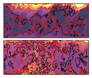
Before turning our attention to statistical and scaling properties of UMZs and UTZs, it is instructive to first consider how the spatial structure of these zones changes with varying thermal instability. Instantaneous snapshots of velocity and temperature in the  $x$–
$x$– $z$ plane at arbitrary times and spanwise locations are plotted in figure 6(a,c,e,g). Here, the black curves indicate UMZ or UTZ interfaces. Corresponding instantaneous velocity and temperature profiles at the locations denoted by the vertical blue lines in panels (a,c,e,g) can be found in figure 6(b,d, f,h). In each panel, the instantaneous velocity or temperature in each UMZ or UTZ is indicated by a black curve, modal values in each zone are given by the blue curves, and grey dashed curves denote ensemble mean values. Panels (a–d) correspond to near-neutral ( $-\delta /L=0.3)$ conditions, while panels (e–h) correspond to highly convective ( $-\delta /L=261$) conditions. In order to illustrate the behaviour of UMZs and UTZs over a streamwise region of extent ${\sim }5 \delta$ (larger than the window size $\mathcal {L}_x = 0.25 \delta$ used in the histogram-based detection of UMZs and UTZs), the fuzzy clustering method (FCM; Fan et al. Reference Fan, Xu, Yao and Hickey2019) was employed in figures 6–7 to calculate UMZs and UTZs. The FCM has been found to identify similar zones as the histogram-based method, given the same number of zones. We calculated the number of UMZs and UTZs in each streamwise window of size $\mathcal {L}_x = 0.25 \delta$, and then mean number of zones over the entire region considered (of streamwise extent $5 \delta$) was used input to the FCM. This is just done for illustration purposes in these figures; UMZ and UTZ statistics are calculated after zone detection using the histogram-based method discussed above.

Figure 6. Examples of UMZs and UTZs from suite of simulations. (a,c,e,g) Instantaneous snapshots in  $x$–
$x$– $z$ plane, (b,d, f,h) instantaneous profiles ( $\tilde {u}/u_\tau$ and $\tilde {\theta }$), stepwise profiles based on modal velocities and temperatures in UMZs and UTZs ( $\tilde {u}_m$ and $\tilde {\theta }_m$) and mean velocity and temperature ( $\bar { \tilde {u} }/u_\tau$ and $\bar { \tilde {\theta }}$). Panels (a–d) are displayed for $-\delta /L=0.30$, and (e–h) for $-\delta /L=261$; (a,b,e, f) depict UMZs for velocity and (c,d,g,h) depict UTZs for temperature.
Under weakly convective conditions (figure 6a), UMZs are organized into inclined structures increasing in depth in the downstream direction, consistent with previous findings in turbulent boundary layers (Meinhart & Adrian Reference Meinhart and Adrian1995; Adrian et al. Reference Adrian, Meinhart and Tomkins2000; de Silva et al. Reference de Silva, Hutchins and Marusic2016). The instantaneous streamwise velocity in panel (b) exhibits the characteristic stair-step pattern reported by previous authors (de Silva et al. Reference de Silva, Hutchins and Marusic2016, Reference de Silva, Philip, Hutchins and Marusic2017; Heisel et al. Reference Heisel, De Silva, Hutchins, Marusic and Guala2020). For the near-neutral case, one UTZ is found near the ground (figure 6c), with an interface that closely corresponds to UMZ interfaces. Instantaneous temperature profiles (d) decrease with height close to the ground, and then are well mixed with only a couple of discrete UTZs present for  $z/\delta \leqslant 0.8$ in this particular snapshot. However, a stair-step pattern, with large jumps in temperature can be observed in the entrainment zone (e.g. $z/\delta \geqslant 0.8$).
For highly convective conditions, UTZs encompass thermal plumes (figure 6g). However, here, the spatial structure of UMZs (panel e) is very different than that of UTZs, forming regions of alternating high and low streamwise momentum, due to horizontal convergence and divergence into the updrafts and downdrafts (e.g. Salesky et al. Reference Salesky, Chamecki and Bou-Zeid2017). In contrast to the stair-step pattern observed in the instantaneous velocity profile for the weakly convective case,  $\tilde {u}/u_\tau$ here exhibits alternating positive and negative jumps with increasing height throughout the mixed layer (figure 6f). However, the instantaneous temperature profile remains qualitatively similar to the weakly convective case. Note that negative interfacial jumps ( $\Delta u, \Delta \theta < 0$) constitute local gradients that oppose the mean velocity and temperature gradients. Physically, the alternating positive and negative velocity and temperature jumps in the mixed layer are consistent with what is known about properties of thermal plumes in the convective mixed layer (e.g. Deardorff Reference Deardorff1972; Schmidt & Schumann Reference Schmidt and Schumann1989; Moeng & Sullivan Reference Moeng and Sullivan1994; Khanna & Brasseur Reference Khanna and Brasseur1998). The instantaneous structure of the mixed layer is composed of both updrafts (where $w'>0$, $\theta '>0$, and $u'<0$) and downdrafts (where $w'<0$, $\theta '<0$, and $u'>0$). Both updrafts and downdrafts coexist in the mixed layer, necessitating both positive and negative interfacial velocity and temperature jumps as a local and instantaneous velocity or temperature profile intersects high- and low-momentum and temperature regions. Statistical properties of these velocity and temperature jumps will be discussed further in § 3.4.
A more direct comparison between UMZ and UTZ interfaces as a function of stability can be found in figure 7. Here, streamwise velocity is plotted in the left panels and temperature in the right panels using filled colour contours, with black and red curves denoting UMZ and UTZ interfaces, respectively. Panels include flow visualizations for (a,b)  $-\delta /L = 0.3$, (c,d) $-\delta /L=9.2$, and (e, f) $-\delta /L=261$. For the near-neutral case in panels (a,b), there is noticeable similarity between the UTZ interface detected in the surface layer (e.g. for $z/\delta \leqslant 0.1$) and the UMZ interfaces. This indicates that the coherent structures transporting momentum and heat are similar under near-neutral thermal stratification. The UMZ and UTZ interfaces are also very similar in the entrainment zone (e.g. $z/\delta \geqslant 0.8$), indicative of coinciding zones of quasi-uniform momentum and temperature. For the $-\delta /L=9.8$ case (panels c,d), there still is similarity between the UMZ and UTZ interfaces. Here, one can see that regions of low-momentum warm fluid are being uplifted from the ground due to buoyancy. While there is not perfect agreement between UMZ and UTZ interfaces, some corresponding features can be observed in both the streamwise momentum and temperature fields. For the most highly convective case ( $-\delta /L=261$, panels e, f), there is a marked difference between the UMZ and UTZ interfaces. As buoyancy forcing increases, the horizontal momentum field is driven primarily by convergence and divergence into and out of buoyant updrafts and downdrafts. Here, warm updrafts are flanked by high- and low-momentum fluid, such that momentum and temperature are out of phase. Thus, under highly convective conditions, the UMZ interfaces deviate from the UTZ interfaces that encompass thermal plumes.

Figure 7. Comparison of UMZ and UTZ interfaces for several stabilities. Filled colour contours are plotted in the  $x$–
$x$– $z$ plane for momentum in panels (a,c,e) and for temperature in (b,d, f). Black and red curves are used to denote UMZ and UTZ interfaces, respectively. Cases are (a,b) $-\delta /L = 0.3$, (c,d) $-\delta /L = 9.2$, (e, f) $-\delta /L = 261$. Grey horizontal lines indicate the outer-normalized Obukhov length magnitude, i.e. $-L/\delta$.
The results presented in figure 7 are consistent with previous findings in the convective boundary layer literature (Li & Bou-Zeid Reference Li and Bou-Zeid2011; Patton et al. Reference Patton, Sullivan, Shaw, Finnigan and Weil2016; Salesky et al. Reference Salesky, Chamecki and Bou-Zeid2017), which have demonstrated a breakdown of Reynolds’ analogy – the assumption that momentum and scalars are transported similarly by turbulence – as  $-\delta /L$ increases. Using in situ ASL observations, Li & Bou-Zeid (Reference Li and Bou-Zeid2011) found significant differences between the momentum flux ( $\overline { u^\prime w^\prime }$) and heat flux ( $\overline { w^\prime \theta ^\prime }$) in the CBL with increasing instability. They hypothesized that these differences were due a transition in coherent structures from hairpin vortices to thermal plumes. A subsequent LES study by Salesky et al. (Reference Salesky, Chamecki and Bou-Zeid2017) found an order of magnitude decrease in the momentum transport efficiency (the downgradient fraction of the total flux) in the ASL, while the heat transport efficiency only varied by 10 % from weakly to highly convective conditions. They also observed – in support of the hypothesis of Li & Bou-Zeid (Reference Li and Bou-Zeid2011) – a concurrent decrease in spanwise vorticity and increase in vertical vorticity with increasing $-\delta /L$, as one would expect if there was a transition from hairpin vortices to vertically dominant thermal plumes. This breakdown of Reynolds analogy with increasing instability can be interpreted in the context of the spatial differences between UMZs and UTZs that are observed in figure 7. Under weakly convective conditions, the UMZ interfaces – which intersect heads of hairpin vortices (Adrian et al. Reference Adrian, Meinhart and Tomkins2000) – and UTZ interfaces are collocated, such that hairpin vortex packets transport momentum and heat in a similar manner. However, as $-\delta /L$ increases, the UTZ interfaces encompass thermal plumes while UMZ organization becomes increasingly influenced by convergence and divergence from updrafts and downdrafts. Thus, distinctly different structural features are found in the streamwise momentum and temperature fields as buoyancy forcing increases, leading to the breakdown of Reynolds’ analogy with increasing $-\delta /L$.
3.4. The UMZ and UTZ statistics
In this section we consider how statistical properties of UMZs and UTZs, including the interfacial velocity and temperature jumps and the depth of the zones, vary with unstable stratification. The UMZs and UTZs were detected using a histogram-based method (discussed in § 2.3), then a stepwise profile was constructed using the modal velocity or temperature in each zone corresponding to the detected local maxima (figure 1 schematic). The modal velocity profile was used to determine mean UMZ depth ( $h_m$) in the wall-normal direction, which was assigned to the height of the UMZ centre $z_{c,m}$ illustrated in figure 1(c). The interfacial velocity jumps were assigned to the wall-normal height of the UMZ interface $z_{i,m}$. This was done for each instantaneous profile, and statistics were calculated by averaging in time and in horizontal planes to obtain vertical profiles of $h_m$ and $\Delta u$ as a function of $z/\delta$. An analogous procedure was used to calculate UTZ statistics. The interfacial velocity and temperature jumps ( $\Delta u$ and $\Delta \theta$) are defined as the difference in the modal velocities (corresponding to the local maxima in histograms) between subsequent UMZs or UTZs.
The mean depths of UMZs and UTZs and the mean interfacial velocity and temperature jumps are displayed in figure 8. The UMZ depth  $h_m$ is plotted as a function of $z/\delta$ in panels (a,b) and UTZ depth $h_\theta$ is plotted in panels (d,e), where the depth of the zones is normalized by the outer length scale $\delta$ in the first column and by height $z$ in the second column. Panels in the right column depict the (c) mean velocity jumps across UMZ interfaces and (d) mean temperature jumps across UTZ interfaces.

Figure 8. Vertical profiles of mean UMZ and UTZ properties. (a) Average depth of UMZs ( $h_m$), normalized by boundary layer depth $\delta$, (b) average depth of UMZs normalized by height $z$, (c) average velocity jump ( $\Delta u$) across UMZ interfaces normalized by shear velocity scale $u_\tau$, (d) average depth of UTZs ( $h_\theta$) normalized by boundary layer depth $\delta$, (e) average depth of UTZs normalized by height $z$, ( f) average temperature jump across UTZ interfaces normalized by shear temperature scale magnitude $|\theta _\tau |$.
Near the ground, the average depth of both UMZs and UTZs is  ${\approx }2 z$ (figure 8b,e). This is consistent with the attached eddy hypothesis (Townsend Reference Townsend1976), which states that the vertical extent of turbulent eddies is regulated by their distance from the wall. However, some caution in interpretation is warranted here, given the influence of the LES wall model on near-wall statistics and uncertainties in the UMZ/UTZ detection technique near the wall. Note that zones are not typically identified for low values of $\tilde {u}/u_\tau$ (e.g. figures 1–2), as these zones do not satisfy all the detection criteria. Future studies using DNS or wall-resolved LES to study near-wall properties of UMZs and UTZs in unstably stratified flows are therefore needed.
The outer-normalized UMZ depth (panel a) is quasi-constant throughout the mixed layer for all stabilities considered, with  $h_m/\delta$ increasing with increasing $-\delta /L$. This relative invariance with height points to similar physical mechanisms being responsible for UMZ generation throughout the mixed layer across the stabilities considered here. Near the ground, the average jump in velocity across UMZ interfaces is $\Delta u \approx 0.5$– $1.0 u_\tau$. In the mixed layer, the velocity jumps are very small ( $\Delta u \approx 0.2 u_\tau$) for the near-neutral case, and are near zero for the more highly convective cases. In the entrainment zone (e.g. $z/\delta \geqslant 0.8$), the velocity jumps again increase to values of $\Delta u \approx 0.4$– $0.5 u_\tau$, due to the region of secondary mean wind shear that is a ubiquitous feature of sheared convective boundary layers (e.g. figure 4a).
For the weakly convective cases ( $-\delta /L = 0.3, 0.8$) the mean UTZ depth (figure 8d,e) attains its maximum value near $z/\delta =0.3\unicode{x2013}0.4$, corresponding to deeper UTZs in the mixed layer. This is consistent with the instantaneous structure of UTZs which can be seen in the flow visualizations in figure 6. Similar behaviour is observed for the more convective cases, except with both maximum zone depth ( $h_\theta /\delta \approx 0.2$) and the height of maximum zone depth increasing with $-\delta /L$. For all stabilities, $\Delta \theta$ is negative in the surface layer, and changes sign around $z/\delta \approx 0.3$ for the weakly convective cases and around $z/\delta \approx 0.5$ for the highly convective cases. The height at which $\Delta \theta / |\theta _\tau |$ changes sign is comparable to the lower boundary of the entrainment zone where $\overline {w'\theta '}$ becomes negative (e.g. figure 4d).
In addition to characterizing mean properties of UMZs and UTZs, it is also useful to consider the distributions of interfacial velocity and temperature jumps. In figure 9, p.d.f.s are presented of (a–d) UMZ interfacial velocity jumps and (e–h) UTZ interfacial temperature jumps. Here, the abscissa corresponds to the normalized variable of interest, the ordinate axis to dimensionless height ( $z/\delta$), and filled colour contours to values of the p.d.f. Several selected stabilities are displayed, specifically $-\delta /L = 0.3$, 0.8, 9.2 and 261 in the columns from left to right.

Figure 9. Probability density functions of UMZ and UTZ properties as a function of dimensionless height ( $z/\delta$). (a–d) Dimensionless velocity jump across UMZ interfaces ( $\Delta u / u_\tau$), (e–h) dimensionless temperature jump across UTZ interfaces ( $\Delta \theta / \lvert \theta _\tau \rvert$); (a,e) $-\delta /L = 0.3$, (b, f) $-\delta /L = 0.79$, (c,g) $-\delta /L = 9.2$, (d,h) $-\delta /L = 261$.
For all stabilities considered here, the most probable interfacial velocity jumps in the surface layer and entrainment zone are positive. However, in the mixed layer, the p.d.f.s of  $\Delta u / u_\tau$ exhibit bimodal behaviour, which is consistent with the alternating positive and negative $\Delta u / u_\tau$ observed from the flow visualizations in figure 6. For the more weakly convective cases ( $-\delta /L=0.3, 0.79, 9.2$), the most probable values of velocity jumps in the mixed layer are $\Delta u \approx \pm 1.0 u_\tau$. The magnitude of the mixed layer velocity jumps increases to $|\Delta u| \approx 2.5 u_\tau$ for the most convective ( $-\delta /L=261$) case. The p.d.f.s of interfacial temperature jumps are consistent with the mean profiles (figure 8f) where the most probable value of $\Delta \theta$ is negative near the surface, positive in the entrainment zone, and exhibits bimodal behaviour in the mixed layer – indicative of alternating positive and negative jumps. The magnitude of the interfacial temperature jumps in the mixed layer decreases with increasingly unstable conditions, from $|\Delta \theta | \approx 2 | \theta _\tau |$ for $-\delta /L=0.3$ to $|\Delta \theta | \approx 0.5 | \theta _\tau |$ for $-\delta /L=261$.
To summarize, we find that in the surface layer, the average depth of UMZs and UTZs is  $\approx 2 z$, consistent with the attached eddy hypothesis, although these results should be interpreted with some caution given the influence of the LES wall model. In the mixed layer, the depth of UMZs approach constant values for a given stability, ranging from $h_m/\delta =0.03\unicode{x2013}0.06$, and increasing with $-\delta /L$. The UTZ depth is at is maximum in the centre of the boundary layer, attaining values of $h_\theta = 0.15 \delta$ to $0.23 \delta$, indicating of a deep zone of quasi-uniform temperature typically present in the centre of the mixed layer. Interfacial velocity jumps are largest in the surface layer and the entrainment zone, and become quite small (e.g. $|\Delta u| < 0.2 u_\tau$) throughout the mixed layer. Interfacial temperature jumps are negative near the ground, positive in the entrainment zone, and change sign at a height that roughly corresponds to the bottom of the entrainment zone (where $\overline {w'\theta '}$ becomes negative. The surface-layer scaling of UMZ and UTZ properties will be considered further in the following section.
3.5. The UMZs, UTZs and scaling laws in the surface layer
We now consider the extent to which UMZ and UTZ properties in the ASL can explain scaling laws for the dimensionless mean velocity and temperature gradients under unstably stratified conditions. A recent paper (Heisel et al. Reference Heisel, De Silva, Hutchins, Marusic and Guala2020) argued that under neutral stratification, UMZs can be linked to the hypothetical turbulent eddies that Prandtl (Reference Prandtl1925) invoked in his derivation of the logarithmic law of the wall. Following Prandtl's arguments, the mean velocity gradient can be written as
 \begin{equation} \frac{\partial \bar{U} }{\partial z} \sim \frac{u_\tau}{\ell_m}. \end{equation}
Here,  $\ell _m$ is the mixing length, which can be interpreted as the characteristic length scale over which turbulent eddies transport momentum. Assuming $\ell _m = \kappa z$ under neutral stratification, (3.1) can be integrated to obtain the log law
 \begin{equation} \frac{\bar{U}}{u_\tau} = \frac{1}{\kappa} \ln z^+ + A_u, \quad z^+ = \frac{z u_\tau}{\nu} , \end{equation}
where  $A_u$ is a constant that depends on the surface roughness.
Heisel et al. (Reference Heisel, De Silva, Hutchins, Marusic and Guala2020) related the scaling of the mean velocity gradient in the inertial sublayer to UMZ properties
 \begin{equation} \frac{\partial \bar{U}}{\partial z} = \frac{u_\tau}{\kappa z} \sim \frac{\Delta u}{h_m}, \end{equation}
where they envisioned the mean gradient as arising due to the collective effects of an ensemble of interfacial velocity jumps ( $\Delta u$) over zones of depth $h_m$. They presented evidence that under neutral stratification the interfacial velocity jumps scale on the friction velocity, $\Delta u \sim u_\tau$, while UMZ depth scales on the neutral mixing length $h_m \sim \ell _m = \kappa z$. In this manner, they linked coherent structures in the flow (i.e. UMZs associated with mean shear) to the log law.
Other authors (Anderson & Salesky Reference Anderson and Salesky2021; Zheng & Anderson Reference Zheng and Anderson2022) have instead suggested that the salient length scale linking UMZs to the mean velocity gradient is the vorticity thickness  $\delta _{\omega }$ (Brown & Roshko Reference Brown and Roshko1974; Chauhan et al. Reference Chauhan, Philip, de Silva, Hutchins and Marusic2014; de Silva et al. Reference de Silva, Philip, Hutchins and Marusic2017; Bautista et al. Reference Bautista, Ebadi, White, Chini and Klewicki2019), defined as
 \begin{equation} \delta_\omega = \frac{ \lvert \Delta u \rvert}{\max \lvert {\partial \langle {U} \rangle }/{\partial z}\rvert}, \end{equation}
where  $\langle {\cdot } \rangle$ denotes a conditional average across a UMZ interface. On physical grounds, this corresponds to shear being concentrated in thin regions of thickness $\delta _\omega$ associated with UMZ interfaces, and negligible shear within each zone. Note that absolute values are used in (3.4) so that $\delta _\omega$ is non-negative by definition. From this perspective, one would expect the mean gradient to scale as
 \begin{equation} \frac{\partial \bar{U}}{\partial z} = \frac{u_\tau}{\ell_m} \sim \frac{\Delta u}{\delta_\omega}. \end{equation}
 One can also invoke mixing length arguments to derive a surface-layer scaling for the mean temperature gradient, by hypothesizing that the mean temperature gradient scales as the ratio of a shear temperature scale  $\theta _\tau$ to the mixing length for heat $\ell _h$
 \begin{equation} \frac{\partial \bar{\theta}}{\partial z} = \frac{\theta_\tau}{\ell_h}. \end{equation}
Using the neutral mixing length  $\ell _h = \kappa z$, one can integrate (3.6) to show that, under near-neutral stratification, the mean temperature profile also follows a log law
 \begin{equation} \frac{\bar{\theta} - \theta_s}{\theta_\tau} = \frac{1}{\kappa} \ln z^+ + A_\theta, \end{equation}
where  $\theta _s$ is surface temperature, and $A_\theta$ is a constant that depends on the surface roughness. From the perspective of UTZs, the equivalent statement to (3.5) is
 \begin{equation} \frac{\partial \bar{\theta}}{\partial z} = \frac{\theta_\tau}{\ell_h} \sim \frac{\Delta \theta}{\delta_{\boldsymbol{\nabla}\theta}}. \end{equation}
That is, one may hypothesize that the mean surface-layer temperature gradient arises due to the ensemble effects of interfacial temperature jumps  $\Delta \theta$ across UTZ interfaces of thickness $\delta _{\boldsymbol {\nabla } \theta }$ and negligible gradients within each UTZ. Through analogy with $\delta _{\omega }$, one may define a temperature gradient thickness $\delta _{\boldsymbol {\nabla } \theta }$
 \begin{equation} \delta_{\boldsymbol{\nabla}\theta} = \frac{ \lvert \Delta \theta \rvert}{\max \lvert \partial \langle {\theta} \rangle/\partial z \rvert} . \end{equation}
 Under thermally stratified conditions, the mean velocity profile (MVP) in the surface layer deviates from the log law due to buoyancy effects. The effects of thermal stratification on the MVP and other turbulence statistics in the ASL can be explained in the context of Monin–Obukhov similarity theory (MOST; Obukhov Reference Obukhov1946; Monin & Obukhov Reference Monin and Obukhov1954), where any turbulence statistic non-dimensionalized using the height  $z$, friction velocity $u_\tau$ and buoyancy parameter $g/\varTheta _0$ and the kinematic surface heat flux $Q_0$ is predicted to be a universal function of the Monin–Obukhov stability variable $\zeta = z/L$. Here, $L$ is the Obukhov length given in (1.1). Thus, under thermally stratified conditions, the dimensionless mean velocity and temperature gradients are predicted be universal functions of $\zeta$
 $$\begin{gather} \frac{\kappa z}{u_\tau} \frac{\partial \bar{U}}{\partial z} = \phi_m(\zeta) , \end{gather}$$
 $$\begin{gather}\frac{\kappa z}{\theta_\tau} \frac{\partial \bar{\theta} }{\partial z} = \phi_h(\zeta). \end{gather}$$
The universal functions  $\phi _m(\zeta )$ and $\phi _h(\zeta )$ must be determined empirically; many formulations are available in the literature (e.g. Businger et al. Reference Businger, Wyngaard, Izumi and Bradley1971; Högström Reference Högström1988; Brutsaert Reference Brutsaert1999). In this article, we use the empirical functions for $\phi _m$ and $\phi _h$ presented by Brutsaert (Reference Brutsaert1999) based on the directional dimensional analysis of Kader & Yaglom (Reference Kader and Yaglom1990). These empirical functions are used because they capture the local free convective scalings $\phi _m(\zeta ) \propto (-\zeta )^{1/3}$ and $\phi _h(\zeta ) \propto (-\zeta )^{-1/3}$ for $-\zeta \gg 1$; additional details can be found in Appendix A.
Following MOST, the mean velocity and temperature gradients under thermally stratified conditions are given as
 \begin{equation} \frac{\partial \bar{U}}{\partial z} = \frac{u_\tau}{\ell_m} = \frac{u_\tau}{\kappa z / \phi_m(\zeta)} \end{equation}
and
 \begin{equation} \frac{\partial \bar{\theta} }{\partial z} = \frac{\theta_\tau}{\ell_h} = \frac{\theta_\tau}{\kappa z / \phi_h(\zeta)}. \end{equation}
In (3.12)–(3.13),  $\ell _m$ and $\ell _h$ are the stability dependent mixing lengths for momentum and temperature, defined as
 $$\begin{gather} \ell_m = \frac{\kappa z }{ \phi_m(\zeta) } \end{gather}$$
 $$\begin{gather}\ell_h = \frac{\kappa z }{ \phi_h(\zeta) }. \end{gather}$$
Because  $\phi _m(\zeta ) < 1$ and $\phi _h(\zeta )<1$ for unstable conditions, the mixing lengths under unstable stratification exceed their neutral values ( $\ell _m > \kappa z$ and $\ell _h > \kappa z$ for $\zeta < 0$), which physically corresponds to enhanced mixing due to the effects of buoyancy-generated turbulence under unstable thermal stratification.
Before examining the linkages between UMZ and UTZ properties and the scaling of the mean velocity and temperature gradients in the atmospheric surface layer following MOST, we first shall consider the surface layer behaviour of the relevant velocity and temperature scales ( $\Delta u$ and $\Delta \theta$) and length scales ( $h_m$, $h_\theta$, $\delta _{\omega }$ and $\delta _{\boldsymbol {\nabla } \theta }$). The shear-normalized interfacial velocity and temperature jumps in the surface layer are displayed in figure 10(a,b). Here, $\Delta u$ and $\Delta \theta$ are only displayed for $z/\delta \geqslant 0.05$ given uncertainty in zone detection and the influence of the LES wall model close to the surface. One can see that when normalized by $u_\tau$, the interfacial velocity jumps in the surface layer (figure 10a) collapse reasonably well to a single curve for all stabilities except for the most convective case ( $-\delta /L=261$). However, the interfacial temperature jumps, displayed in panel (b) do not collapse, but rather exhibit a systematic ordering where $\Delta \theta / \theta _\tau$ decreases monotonically with increasing $-\delta /L$ for a given value of $z/\delta$. Both $\Delta u$ and $\Delta \theta$ decrease with increasing distance from the ground, consistent with previous studies (e.g. de Silva et al. Reference de Silva, Philip, Hutchins and Marusic2017; Heisel et al. Reference Heisel, De Silva, Hutchins, Marusic and Guala2020).

Figure 10. Velocity and temperature jumps across UMZ and UTZ interfaces, respectively, in the surface layer. (a) Interfacial velocity jumps  $\Delta u$, normalized by shear velocity scale $u_\tau$, (b) interfacial temperature jumps $\Delta \theta$, normalized by shear temperature scale $\theta _\tau$.
Surface-layer behaviour of the length scales associated with UMZs and UTZs is illustrated in figure 11, with the panels corresponding to (a) UMZ depth  $h_m$, (b) UTZ depth $h_\theta$, (c) vorticity thickness $\delta _\omega$ and (d) temperature gradient thickness $\delta _{\boldsymbol {\nabla } \theta }$. These length scales associated with UMZs and UTZs are normalized by the stability-dependent mixing lengths for momentum $\ell _m$, and heat $\ell _h$, respectively (3.14)–(3.15). One can see that the curves for different $-\delta /L$ values for $h_m / \ell _m$ begin to collapse above $z/\delta = 0.15$, but exhibit a significant amount of spread closer to the ground. The normalized vorticity thickness (panel c) exhibits better collapse than the UMZ depth for all heights displayed here, except for the most unstable cases ( $-\delta /L = 27.5, 261$), indicating that it is a more appropriate mixing length for momentum than $h_m$ in the surface layer under unstable stratification. Length scales associated with UTZs are displayed in the right panels of figure 11, with UTZ depth in panel (b) and temperature gradient thickness in panel (d). One can see that neither $h_\theta$ or $\delta _{\boldsymbol {\nabla } \theta }$ collapse to a single curve when normalized by $\ell _h$, and both decrease systematically with increasing $-\delta /L$. However, this $-\delta /L$ dependence is comparable to what is found for $\Delta \theta / \theta _\tau$ (figure 10b), suggesting that collapse of the normalized gradients still may be possible.

Figure 11. Behaviour of length scales associated with UMZs and UTZs in the surface layer; (a) UMZ depth  $h_m$, (b) UTZ depth $h_\theta$, (c) vorticity thickness $\delta _\omega$, (d) temperature gradient thickness $\delta _{\boldsymbol {\nabla }\theta }$. Length scales are normalized by the mixing lengths for momentum $\ell _m = \kappa z / \phi _m(\zeta )$ and heat $\ell _h = \kappa z / \phi _h(\zeta )$.
The connection between the mean velocity and temperature gradients in the surface layer and properties of UMZs and UTZs is examined in figure 12. The left panels depict the extent to which the scaling of the surface-layer mean velocity gradient following MOST is related to UMZ properties, with panel (a) considering the scaling  $\partial \bar {U} / \partial z \sim \Delta u / h_m$ and panel (b) considering the scaling $\partial \bar {U} / \partial z \sim \Delta u / \delta _\omega$. In both panels, the gradients based on UMZ properties are normalized by $\ell _m / u_\tau$. If a scaling is appropriate, one would expect collapse of all curves for different stabilities ( $-\delta /L$ values) to an $O(1)$ constant. One can see that both scalings for ${\partial \bar {U} }/{\partial z}$ lead to reasonably good collapse of all curves in panels (a,c). The normalized velocity gradient calculated using $\delta _\omega$ as the length scale in figure 12(c) does exhibit some weak $-\delta /L$ dependence. Note that previous observational and LES studies have found that calculated values of $\phi _m$ exhibit significant scatter and do not collapse as a function of $\zeta$ alone (Khanna & Brasseur Reference Khanna and Brasseur1997; Johansson et al. Reference Johansson, Smedman, Högström, Brasseur and Khanna2001; Salesky & Chamecki Reference Salesky and Chamecki2012). These deviations from Monin–Obukhov similarity have been explained by taking $-\delta /L$ as an additional scaling parameter (Khanna & Brasseur Reference Khanna and Brasseur1997; Johansson et al. Reference Johansson, Smedman, Högström, Brasseur and Khanna2001) and by accounting for the large-scale velocity due to LSMs in dimensional analysis (Salesky & Anderson Reference Salesky and Anderson2020a). The amount of scatter in scalings based on $h_m$ and $\delta _\omega$ can be quantified by considering the coefficient of variation $c_v$, defined as
 \begin{equation} c_v = \frac{\sigma(z/\delta)}{\mu(z/\delta)}, \end{equation}
that is, the ratio of the standard deviation to mean of the normalized gradients, where both  $\mu$ and $\sigma$ are taken across the seven different $-\delta /L$ values considered here. Smaller values of $c_v$ indicate better collapse to a single curve (i.e. less scatter). One can see from figure 12(e) that while using $h_m$ or $\delta _\omega$ yield similar values of $c_v$ at some heights, overall employing $\delta _\omega$ as a length scale leads to better collapse of the normalized mean velocity gradient on average throughout the ASL.

Figure 12. Surface-layer scaling of mean velocity and temperature gradients based on UMZ and UTZ properties. (a) Mean velocity gradient based on interfacial velocity jumps and UMZ depth  $\Delta u / h_m$. (b) Mean temperature gradient based on interfacial temperature jumps and UTZ depth $\Delta \theta / h_\theta$. (c) Mean velocity gradient based on interfacial velocity jumps and vorticity thickness $\Delta u / \delta _\omega$. (d) Mean temperature gradient based on interfacial temperature jumps and temperature gradient thickness $\Delta \theta / \delta _{\boldsymbol {\nabla } \theta }$. Mean gradients are normalized by shear velocity and temperature scales ( $u_\tau$ and $\theta _\tau$), and stability-dependent mixing lengths for momentum and heat ( $\ell _m$ and $\ell _h$). Panels (e–f) include the coefficients of variation (3.16) for the curves in panels (a–d), indicative of the level of collapse to a single curve for the different scalings.
Surface-layer scaling of the mean temperature gradient based on UTZ properties is considered in the right panels of figure 12, with normalization based on UTZ depth in panel (b), normalization based on temperature gradient thickness in (d) and profiles of  $c_v$ in ( f). One can see that the scaling based on UTZ depth ( $\partial \bar {\theta } / \partial z \sim \Delta \theta / h_\theta$), considered in panel (b) exhibits significantly more scatter than the scaling based on temperature gradient thickness ( $\partial \bar {\theta } / \partial z \sim \Delta \theta / \delta _{\boldsymbol {\nabla } \theta }$) in panel (d). This is further supported by the coefficient of variation profiles in panel ( f). Physically, this indicates that the temperature gradient thickness $\delta _{\boldsymbol {\nabla }\theta }$ is a more appropriate mixing length for temperature than $h_\theta$, which is consistent of the picture of gradients being predominately concentrated across UTZ interfaces and occurring over length $\delta _{\boldsymbol {\nabla }\theta }$.
While scalings for the surface-layer mean velocity and temperature gradients  $\partial \bar {U} / \partial z \sim \Delta u / \delta _{\omega }$ and $\partial \bar {\theta } / \partial z \sim \Delta \theta / \delta _{\boldsymbol {\nabla } \theta }$ exhibit reasonable collapse to a single curve for all stabilities when normalized by the mixing lengths ( $\ell _m$ and $\ell _h$), and shear velocity and temperature scales ( $u_\tau$ and $\theta _\tau$), there is still a weak $z/\delta$ dependence observed within the surface layer. While the empirical Businger–Dyer curves (Dyer Reference Dyer1974) also were considered (which follow $\phi _m \propto (-\zeta )^{-1/4}$ and $\phi _h \propto (-\zeta )^{-1/2}$ scaling behaviour for weakly convective conditions), we found that the empirical MOST functions from Brutsaert (Reference Brutsaert1999) (based on Kader & Yaglom Reference Kader and Yaglom1990) lead to superior collapse of the normalized gradients. Evidently, it is important to account for local free convective scaling ( $\phi _m \propto (-\zeta )^{1/3}$ and $\phi _h \propto (-\zeta )^{-1/3}$) for $-\zeta \gg 1$. In summary, these results provide evidence of the connection between uniform momentum and temperature zones with interfacial velocity and temperature jumps ( $\Delta u$ and $\Delta \theta$ ) across regions of thickness $\delta _\omega$ and $\delta _{\boldsymbol {\nabla } \theta }$ contributing to the observed scaling behaviour of the ASL mean velocity and temperature gradients following MOST.
3.6. Conditionally averaged profiles
In this section we consider the relationship between turbulent fluxes (viewed through the lens of quadrant analysis), UMZs and UTZs using conditional averaging. Previous work in turbulent boundary layers (e.g. Eisma et al. Reference Eisma, Westerweel, Ooms and Elsinga2015; de Silva et al. Reference de Silva, Philip, Hutchins and Marusic2017; Chen, Chung & Wan Reference Chen, Chung and Wan2021) has revealed that sharp changes occur in both streamwise and wall-normal momentum across UMZ interfaces, such that ejections of momentum (Q2, where  $u^\prime < 0$ and $w^\prime > 0$) are found below the interface and sweeps of momentum (Q4, where $u^\prime > 0$ and $w^\prime < 0$) are found above the interface. de Silva et al. (Reference de Silva, Philip, Hutchins and Marusic2017) noted that their findings were consistent with UMZ interfaces intersecting the heads of hairpin vortices (Adrian et al. Reference Adrian, Meinhart and Tomkins2000). We here consider how this picture is influenced by unstable stratification, examining conditionally averaged $u$,
$u$,  $w$, and $\theta$ profiles across both UMZ and UTZ interfaces.
Figure 13 presents conditionally averaged velocity and temperature profiles, e.g.  $(\overline {u - u_{i,m}})/u_\tau$ where $u_{i,m}$ is the streamwise velocity component at the UMZ interface. Profiles are plotted in a local coordinate system as a function of $(z - z_{i,m})/\delta$, where $z_{i,m}$ is the wall-normal distance to a UMZ interface, at several selected stabilities ( $-\delta /L =$ 0.3, 9.2, 261), and in bins of $z/\delta$. Note that UMZ and UTZ interfaces at heights lower than $z/\delta = 0.05$ were omitted from averaging for the lowest bin to ensure that a sufficient number of points above the ground were available to include in conditional averages and to avoid results being influenced by the LES wall model. Lower in the boundary layer, the region below the UMZ interface is, in an average sense, characterized by negative streamwise velocity fluctuations ( $u'<0$), positive vertical velocity fluctuations ( $w'>0$) and positive temperature fluctuations ( $\theta '>0$), while region above the UMZ interface corresponds to $u'>0$, $w'<0$, and $\theta '<0$. From the perspective of quadrant analysis, this corresponds to ejections of momentum (Q2) and warm updrafts (Q1, $w'>0$ and $\theta '>0$) below the interface, and sweeps of momentum (Q4) and cold downdrafts (Q3, $w'<0$ and $\theta '<0$) above the interface.

Figure 13. Conditionally averaged velocity and temperature profiles across UMZ interfaces; (a–c)  $-\delta /L = 0.30$, (d–f) $-\delta /L = 9.2$, (g–i) $-\delta /L = 261$. (a,d,g) Conditionally averaged streamwise velocity $(\overline { u - u_{i,m} })/u_\tau$; (b,e,h) conditionally averaged wall-normal velocity $( \overline { w - w_{i,m} })/w_\star$; (c, f,i) conditionally averaged potential temperature $(\overline { \theta - \theta _{i,m} } )/\lvert \theta _\star \rvert$. Profiles are displayed in a coordinate system local to UMZ interfaces, i.e. as a function of $( z - z_{i,m} )/\delta$, where $z_{i,m}$ is the height of the UMZ interface. Each curve is plotted for UMZ interfaces lying within the range of $z/\delta$ values indicated in the legend.
For the weakly stable ( $-\delta /L=0.3$) case, the conditionally averaged temperature gradient changes sign as $z/\delta$ increases, consistent with the deep entrainment zone (beginning around $z/\delta =0.4$) that can be seen in figure 4(d). For the $-\delta /L=$ 9.2 and 261 cases, higher in the boundary layer (e.g. $z/\delta =0.5$) the conditionally averaged streamwise velocity and temperature profiles become nearly constant with height. Recall that in the mixed layer, $\Delta u \rightarrow 0$, and the velocity jumps have a bimodal distribution with both positive and negative peaks (figure 9i–l). Thus although instantaneous velocity jumps across UMZ interfaces may be either positive or negative, the conditionally averaged profiles tend towards zero.
A plot of conditional averages relative to the UTZ interfaces is presented in figure 14. Here, we observe the conditionally averaged velocity and temperature profiles across the UTZ interfaces are very similar to what is found for the UMZ interfaces. In the surface layer, ejections of momentum (Q2) and warm updrafts (Q1) occur below UTZ interfaces while sweeps of momentum (Q4) and cold downdrafts (Q3) are found above the UTZ interfaces. Higher in the boundary layer, the conditionally averaged streamwise velocity and temperature profiles tend toward zero, particularly for the  $-\delta /L=9.2$ and 261 cases. Again, these results are consistent with mean UTZ properties and their PDFs (figures 8, 9). Although one might expect significant differences between the conditional averages across UMZ vs UTZ interfaces, we find that both of these types of interfaces have a similar association with the spatial structure of momentum and heat fluxes above and below the interface, with similar variation in the wall-normal direction and with stability.

Figure 14. Conditionally averaged velocity and temperature profiles across UTZ interfaces; (a–c)  $-\delta /L = 0.30$, (d–f) $-\delta /L = 9.2$, (g–i) $-\delta /L = 261$. (a,d,g) Conditionally averaged streamwise velocity $(\overline { u - u_{i,\theta } })/u_\tau$; (b,e,h) conditionally averaged wall-normal velocity $(\overline { w - w_{i,\theta } })/w_\star$; (c,f,i) conditionally averaged potential temperature $(\overline { \theta - \theta _{i,\theta } })/\lvert \theta _\star \rvert$. Profiles are displayed in a coordinate system local to UTZ interfaces, i.e. as a function of $( z - z_{i,m} )/\delta$, where $z_{i,m}$ is the height of the UMZ interface. Each curve is plotted for UTZ interfaces lying within the range of $z/\delta$ values indicated in the legend.
4. Conclusions
Since the pioneering work of Meinhart & Adrian (Reference Meinhart and Adrian1995), UMZs (Meinhart & Adrian Reference Meinhart and Adrian1995; Adrian et al. Reference Adrian, Meinhart and Tomkins2000; de Silva et al. Reference de Silva, Hutchins and Marusic2016, Reference de Silva, Philip, Hutchins and Marusic2017) have been an active topic of research in wall-bounded turbulent shear flows, as they have been found to be linked to the spatial structure of turbulent fluxes (de Silva et al. Reference de Silva, Philip, Hutchins and Marusic2017; Heisel et al. Reference Heisel, Dasari, Liu, Hong, Coletti and Guala2018), scaling laws in the logarithmic region (Heisel et al. Reference Heisel, De Silva, Hutchins, Marusic and Guala2020) and other coherent structures in the flow (e.g. hairpin vortex packets; Adrian et al. Reference Adrian, Meinhart and Tomkins2000). Despite many advances in our understanding of UMZs in turbulent shear flows, the effects of unstable thermal stratification on UMZ structure and the extent to which temperature, an active scalar, organizes into analogous UTZs, have not been explored previously.
In the present work, we have used a suite of LES cases spanning global instability parameters ( $-\delta /L$) of nearly three orders of magnitude to investigate properties of UMZs and UTZs in the convective atmospheric boundary layer. Under weakly unstable stratification, UMZs are organized as ramp-like structures inclined in the downstream direction, as found previously in neutrally stratified flows. In instantaneous flow visualizations, one large UTZ is frequently found spanning much of the convective mixed layer (e.g. $z/\delta \in [0.2,0.8]$) with other distinct zones found in the surface layer and entrainment zone. Even larger structural differences arise between UMZs and UTZs with increasing $-\delta /L$: UTZs predominantly encompass thermal plumes, while UMZs form regions of alternating high- and low-momentum fluid due to horizontal convergence and divergence from thermally generated updrafts and downdrafts.
An examination of statistical properties of UMZs and UTZs reveals that mean zone depth for UMZs is quasi-constant with increasing wall-normal distance, while mean UTZ depth reaches its maximum value of  $h_\theta /\delta = 0.15\unicode{x2013}0.20$ in the centre of the mixed layer ( $z/\delta =0.4\unicode{x2013}0.5$) for all stabilities considered herein. Interfacial average velocity jumps across UMZ interfaces were found to be $\Delta u \approx 0.5\unicode{x2013}1.0 u_\tau$ near the ground, decreasing with height to become smaller in the mixed layer. The p.d.f.s of interfacial velocity jumps and instantaneous profiles reveal that in the mixed layer, instantaneous velocity follows alternating positive and negative jumps across UMZ interfaces with increasing height. Interfacial temperature jumps were found to be $\Delta \theta \approx -1.0 \theta _\tau$ near the ground, and change sign at a height that roughly corresponds to the bottom of the entrainment zone (where $\overline {w'\theta '} < 0$). The observed mean structure of the convective mixed layer, with well-mixed temperature and velocity profiles can be viewed as a consequence of UMZs and UTZs, given the alternating positive and negative temperature jumps in this region (which are small or near zero in an ensemble mean sense).
Connections between UMZ and UTZ properties and scaling laws for the mean velocity and temperature gradients in the surface layer were examined in the context of MOST. When normalized by the friction velocity and stability-dependent mixing length for momentum, the velocity gradient based on UMZ interfacial velocity jumps and vorticity thickness ( $\Delta u / \delta _\omega$) exhibits good collapse the surface layer for all stabilities, establishing a link between UMZ structure and scaling of the mean velocity gradient following MOST under unstably stratified conditions. A corresponding analysis for temperature demonstrates a clear connection between UTZ interfacial temperature jumps ( $\Delta \theta$) and temperature gradient thickness ( $\delta _{\boldsymbol {\nabla } \theta }$) and the surface-layer scaling for $\partial \bar {\theta } / \partial z$ predicted by MOST. Conditionally averaged profiles across UMZ and UTZ interfaces indicate that in the surface layer these interfaces are associated with ejections of momentum and warm updrafts below the interface and sweeps of momentum and cool downdrafts below the interface. Our results reveal that uniform momentum and temperature zones in these unstably stratified flows are closely linked to mean boundary layer structure, instantaneous turbulent fluxes and scaling laws for the mean velocity and temperature profiles in the ASL.
Acknowledgements
The author thanks the four anonymous reviewers for their thoughtful and constructive feedback on this manuscript.
Funding
This work was supported by the US Department of Energy Atmospheric System Research Program, grant no. DE-SC0022124.
Declaration of interests
The author reports no conflict of interest.
Appendix A
In this article, we employ the empirical forms of the universal functions  $\phi _m(\zeta )$ and $\phi _h(\zeta )$ presented in Brutsaert (Reference Brutsaert1999). These functions are smooth interpolants of the scaling regimes presented in Kader & Yaglom (Reference Kader and Yaglom1990), who supposed that the convective ASL can be subdivided into three distinct sublayers (dynamic, dynamic-convective and free-convective) and obtained scaling laws for each via directional dimensional analysis. Specifically, Kader & Yaglom (Reference Kader and Yaglom1990) showed their data were well described by the following functions:
 $$\begin{gather} \phi_m(\zeta) = \begin{cases} 1.04, & -0.04 \leqslant \zeta \leqslant 0 \\ 0.501 (-\zeta)^{{-}1/3}, & -1.2 \leqslant \zeta \leqslant -0.12 \\ 0.380 (-\zeta)^{1/3}, & \zeta \leqslant -2 \end{cases} \end{gather}$$
 $$\begin{gather}\phi_h(\zeta) = \begin{cases} 0.96, & -0.04 \leqslant \zeta \leqslant 0 \\ 0.324 (-\zeta)^{{-}1/3}, & -1.2 \leqslant \zeta \leqslant -0.12 \\ 0.265 (-\zeta)^{{-}1/3}, & \zeta \leqslant -2 \end{cases}. \end{gather}$$
These empirical functions capture near-neutral and local free convective scaling behaviour (e.g. Wyngaard Reference Wyngaard2010)  $\phi _m \propto (-\zeta )^{1/3}$ and $\phi _h \propto (-\zeta )^{-1/3}$ for $-\zeta \gg 1$, whereas other commonly used empirical functions such as the Businger-Dyer curves (Businger et al. Reference Businger, Wyngaard, Izumi and Bradley1971) are typically only considered to be valid for $-2 \leqslant \zeta \leqslant 0$. The interpolation formulas presented by Brutsaert (Reference Brutsaert1999) are given as
 $$\begin{gather} \phi_m(\zeta) = \frac{a + b (-\zeta)^{m + 1/3}}{a + (-\zeta)^m} \end{gather}$$
 $$\begin{gather}\phi_h(\zeta) = \frac{c + d (-\zeta)^{n}}{c + (-\zeta)^n}, \end{gather}$$
with the constants  $a=0.33$, $b=0.41$, $m=1.0$, $c=0.33$, $d=0.057$, and $n=0.78$.


 Open access