


1. Introduction
The fluids in stellar convection zones are generally characterized by a low microscopic Prandtl number,  $\textit {Pr} = \nu /\chi$, where $\nu$ is the kinematic viscosity and $\chi$ is the thermal diffusivity (e.g. Ossendrijver Reference Ossendrijver2003; Augustson, Brun & Toomre Reference Augustson, Brun and Toomre2019). Typical values in the bulk of the solar convection zone, for example, range between $10^{-6}$ and $10^{-3}$ (Schumacher & Sreenivasan Reference Schumacher and Sreenivasan2020). Recently, several studies have explored the possibility that solar convection operates at a high effective Prandtl number regime, meaning that the turbulent Prandtl number $\textit {Pr}_{t}$ exceeds unity (e.g. O'Mara et al. Reference O'Mara, Miesch, Featherstone and Augustson2016; Bekki, Hotta & Yokoyama Reference Bekki, Hotta and Yokoyama2017; Karak, Miesch & Bekki Reference Karak, Miesch and Bekki2018), as a possible solution to the too high velocity amplitudes in simulations in comparison to the Sun (e.g. Hanasoge, Duvall & Sreenivasan Reference Hanasoge, Duvall and Sreenivasan2012; Schumacher & Sreenivasan Reference Schumacher and Sreenivasan2020). However, few attempts have been made to actually measure the turbulent Prandtl number from simulations. A notable exception is the study of Pandey, Schumacher & Sreenivasan (Reference Pandey, Schumacher and Sreenivasan2021), who reported that the turbulent Prandtl number decreases steeply as a function of the molecular Prandtl number, so that $\textit {Pr}_{t} \propto \textit {Pr}^{-1}$ in simulations of standard Boussinesq and variable-heat-conductivity Boussinesq convection. Similar results have recently been reported by Tai et al. (Reference Tai, Ching, Zwirner and Shishkina2021) and Pandey et al. (Reference Pandey, Krasnov, Schumacher, Samtaney and Sreenivasan2022a).
The difficulty in measuring turbulent diffusivities in the absence of large-scale gradients has led to the development of combined eddy-diffusivity mass-flux approaches in convective boundary layers (Siebesma, Soares & Teixeira Reference Siebesma, Soares and Teixeira2007). Here we instead set out to measure turbulent viscosity and thermal diffusivity from a simpler system of isotropically forced homogeneous turbulence. This is done by imposing large-scale gradients of velocity and temperature (equivalently specific entropy) and measuring the response of the system. The turbulent diffusion coefficients are computed from the Boussinesq ansatz and an analogous expression for the enthalpy flux. This method provides a direct measurement of the diffusion coefficients without the need to resort to turbulent closures. Similar methods were used recently to measure the turbulent magnetic Prandtl number (Käpylä et al. Reference Käpylä, Rheinhardt, Brandenburg and Käpylä2020). We compare our results with those from the widely used  $k{-}\epsilon$ model, which was also used by Pandey et al. (Reference Pandey, Schumacher and Sreenivasan2021). We show that the direct results and those from the $k{-}\epsilon$ model are systematically different and that the latter yields misleading results in the flows studied here.
2. The model
We model isotropically forced, non-isothermal turbulence in a fully periodic cube of volume  $(2{\rm \pi} )^3$. We solve the equations of fully compressible hydrodynamics
 \begin{gather} \frac{{\rm D} \ln \rho}{{\rm D} t} ={-}\boldsymbol{\nabla} \boldsymbol{\cdot} {\boldsymbol{u}}, \end{gather}
 \begin{gather}\frac{{\rm D}{\boldsymbol{u}}}{{\rm D} t} ={-}\frac{1}{\rho}(\boldsymbol{\nabla} p - \boldsymbol{\nabla}\boldsymbol{\cdot} 2 \nu \rho {\boldsymbol{\mathsf{S}}}) + {\boldsymbol{f}} - \frac{1}{\tau}({\boldsymbol{u}} - \boldsymbol{\bar{u}}{}_0) , \end{gather}
 \begin{gather}T \frac{{\rm D} s}{{\rm D} t} ={-}\frac{1}{\rho}\left(\boldsymbol{\nabla}\boldsymbol{\cdot}{\boldsymbol{\mathcal{F}}} {}_{rad}-{\mathcal{C}} \right) + 2 \nu \boldsymbol{\mathsf{S}}^2 - \frac{T}{\tau}(s - \bar s_0), \end{gather}
where  ${\rm D}/{\rm D}t = \partial /\partial t + {\boldsymbol {u}}\boldsymbol {\cdot}\boldsymbol {\nabla }$ is the advective derivative, $\rho$ is the density, ${\boldsymbol {u}}$ is the velocity, $p$ is the pressure, $\nu$ is the kinematic viscosity, $\boldsymbol{\mathsf{S}}$ is the traceless rate-of-strain tensor with
 \begin{equation} {\mathsf{S}}_{ij} = {\textstyle{1\over2}} (u_{i,j} + u_{j,i}) - {\textstyle{1\over3}} \delta_{ij} \boldsymbol{\nabla}\boldsymbol{\cdot}{\boldsymbol{u}},\end{equation} ${\boldsymbol {f}}$ is the external forcing, $\tau$ is a relaxation timescale and $\boldsymbol {\bar{u}}{}_0$ is the target mean velocity profile. Furthermore, $T$ is the temperature, $s$ is the specific entropy, ${\boldsymbol{\mathcal {F}}} {}_{rad}$ is the radiative flux, ${\mathcal {C}}$ is a cooling term and $\bar s_0$ is the target mean specific entropy profile. Radiation is modelled via the diffusion approximation, with the radiative flux given by
 \begin{equation} {\boldsymbol{\mathcal{F}}} {}_{rad} ={-}c_{P} \rho \chi \boldsymbol{\nabla} T, \end{equation}
where  $c_{P}$ is the specific heat in constant pressure and $\chi$ is the thermal diffusivity. The ideal gas equation of state $p=(c_{P} - c_{V}) \rho T ={\mathcal {R}} \rho T$ is assumed, where ${\mathcal {R}}$ is the gas constant and $c_{V}$ is the specific heat capacity at constant volume. In a non-isothermal system with forcing and/or imposed large-scale flow, viscous dissipation of kinetic energy acts as a source for thermal energy and leads to a linear increase of the temperature. Additional volumetric cooling is applied to counter this with
 \begin{equation} {\mathcal{C}}({\boldsymbol{x}}) = \rho c_{P} \frac{T({\boldsymbol{x}}) - \langle T_0 \rangle}{\tau_{cool}}, \end{equation}
where  $\langle T_0 \rangle$ is the volume-averaged initial temperature and $\tau _{cool}$ is a cooling timescale. We use $\tau = \tau _{cool} = (c_{s0}k_1)^{-1}$, where $c_{s0}$ is the initial uniform value of the sound speed and $k_1$ is the wavenumber corresponding to the box scale.
The external forcing is given by
 \begin{equation} {\boldsymbol{f}} = {\rm Re}\{ N(t) {\boldsymbol{f}}_{{\boldsymbol{k}}(t)} \exp[{\rm i} {\boldsymbol{k}}(t)\boldsymbol{\cdot} {\boldsymbol{x}} - {\rm i}\phi(t)]\} \end{equation}
(see Brandenburg Reference Brandenburg2001), where  ${\boldsymbol {x}}$ is the position vector and $N(t)= f_0 c_{s} (k(t)c_{s}/\delta t)^{1/2}$ is a normalization factor in which $f_0$ is the forcing amplitude, $k=|{\boldsymbol {k}}|$, $\delta t$ is the length of the time step, and $-{\rm \pi} < \phi (t) < {\rm \pi}$ is a random delta-correlated phase. The vector ${\boldsymbol {f}}_{\boldsymbol {k}}$ describes non-helical transverse waves and is given by
 \begin{equation} {\boldsymbol{f}}_{\boldsymbol{k}} = \frac{{\boldsymbol{k}} \times \hat{\boldsymbol{e}}}{\sqrt{ {\boldsymbol{k}}^2 - ({\boldsymbol{k}} \boldsymbol{\cdot} \hat{\boldsymbol{e}})^2 }}, \end{equation}
where  $\hat {\boldsymbol {e}}$ is an arbitrary unit vector, and where the wavenumber ${\boldsymbol {k}}$ is randomly chosen. The target profiles of mean velocity and specific entropy are given by
 \begin{gather} \boldsymbol{\bar{u}}{}_0 = u_0\sin(k_1 z){\hat{\boldsymbol{e}} {}}_y, \end{gather}
 \begin{gather}\bar s_0 = s_0 \sin(k_1 z). \end{gather}
The imposed mean flow is sufficiently weak so that the turbulence remains nearly isotropic and turbulence production due to the shear is negligible. In addition to the physical diffusion, the advective terms in (2.1) to (2.3) are implemented in terms of fifth-order upwinding derivatives with sixth-order hyperdiffusive corrections and flow-dependent diffusion coefficients; see appendix B of Dobler, Stix & Brandenburg (Reference Dobler, Stix and Brandenburg2006).
The Pencil Code (Pencil Code Collaboration et al. 2021) (http://github.com/pencil-code), which uses high-order finite differences for spatial and temporal discretization, was used to produce the numerical simulations.
2.1. Units, system parameters and diagnostics
The equations are non-dimensionalized by choosing the units
 \begin{equation} [x] = k_1^{{-}1},\quad [\rho] = \rho_0,\quad [u] = c_{s0},\quad [s] = c_{P}, \end{equation}
where  $\rho _0$ is the initial uniform density and $c_{s0} = \sqrt {\gamma {\mathcal {R}} T_0}$ is the sound speed corresponding to the initial temperature $T_0$. The level of velocity fluctuations is determined by the forcing amplitude $f_0$ along with the kinematic viscosity. A key system parameter is the ratio of kinematic viscosity and thermal diffusion or the Prandtl number
 \begin{equation} \textit{Pr} = \frac{\nu}{\chi}, \end{equation}
which is varied between  $0.01$ and $10$ in the present study. The Reynolds and Péclet numbers quantify the level of turbulence of the flows:
 \begin{equation} \textit{Re} = \frac{u_{rms}}{\nu k_{f}},\quad \textit{Pe} = \textit{Pr}\textit{Re} = \frac{u_{rms}}{\chi k_{f}}, \end{equation}
where  $u_{rms} = \sqrt {\langle ({\boldsymbol {u}} - \bar {\boldsymbol {u}}_0)^2 \rangle }$ is the volume-averaged fluctuating root mean square velocity and $k_{f}$ is the average forcing wavenumber characterizing the energy injection scale. The latter is chosen from a uniformly distributed narrow range in the vicinity of $5k_1$. The imposed gradients of large-scale flow and entropy are quantified by
 \begin{equation} \textit{Ma}_s = \frac{u_0}{c_{s0}}, \quad \textit{Ma}_g = \frac{[(\gamma-1)s_0 T_0]^{1/2}}{c_{s0}}, \end{equation}
where  $\textit {Ma}_s$ is the Mach number of the mean flow. The Mach number of the turbulent flow is given by
 \begin{equation} \textit{Ma} = \frac{u_{rms}}{\langle c_{s} \rangle}, \end{equation}
where  $\langle c_{s} \rangle$ is the volume-averaged speed of sound.
Mean values are taken to be horizontal averages denoted by bars; that is,
 \begin{equation} \bar f = \frac{1}{(2{\rm \pi})^2} \int_x \int_y f({\boldsymbol{x}})\,{{\rm d}\kern0.06em x}\, {{\rm d} y}. \end{equation}
Often an additional time average over the statistically steady part of the simulation is taken. Volume averages are denoted by angle brackets  $\langle. \rangle$, apart from the root mean square values, which are always assumed to be volume-averaged unless otherwise stated. Errors were estimated by dividing the time series into three parts and averaging over each subinterval. The greatest deviation from the average computed over the whole time series was taken as the error estimate.
3. Results
The simulations discussed in the present study are listed in table 1.
Table 1. Summary of runs. Runs with imposed velocity or specific entropy gradients are denoted by the prefix i, whereas decay experiments of velocity (specific entropy) are identified by the prefix du (ds). Grid resolutions range between  $144^3$ and $1152^3$.

3.1. Turbulent viscosity and heat diffusion from imposed flow and entropy methods
We measure the turbulent viscosity and thermal diffusivity using large-scale gradients of  ${\boldsymbol {u}}$ and $s$ in two ways. First, we impose sinusoidal large-scale profiles of velocity (2.9) or entropy (2.10). The response of the system consists of non-zero Reynolds stress and vertical enthalpy flux profiles that are parameterized with gradient diffusion terms (e.g. Rüdiger Reference Rüdiger1989),
 \begin{equation} {F^{enth}_z}(z) = c_{P} \overline{(\rho u_z)' T'} \approx c_{P} \bar \rho \overline{u_z' T'} ={-}\chi_{t} \bar \rho \bar T \frac{\partial \bar s}{\partial z} \end{equation}
and
 \begin{equation} {R_{yz}}(z) = \overline{u_y'u_z'} ={-}\nu_{t} \frac{\partial \bar u_y}{\partial z}, \end{equation}
where primes denote fluctuations from the mean, e.g.  ${\boldsymbol {u}}' = {\boldsymbol {u}} - \bar {\boldsymbol {u}}$. The Mach number in the current simulations is always less than 0.1. Therefore we neglect density-dependent terms in our analysis, because they scale with $\textit {Ma}^2$.
The coefficients  $\chi _{t}$ and $\nu _{t}$ are assumed to be scalars and were obtained from linear fits between time-averaged ${F^{enth}_z}$ and $-\bar \rho \bar T\partial _z\bar s$ and between ${R_{yz}}$ and
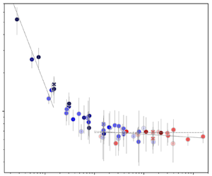
  $-\partial _z \bar u_y$, respectively. Results from our simulations are shown in figure 1. We normalize $\nu _{t}$ and $\chi _{t}$ by
 \begin{equation} \nu_{t0} = \chi_{t0} = {\textstyle{1\over3}}u_{rms}k_{f}^{{-}1}, \end{equation}
which is an order-of-magnitude estimate for the turbulent diffusion coefficients. We note that in the parameter regimes studied here, the estimates  $\nu _{t0}$ and $\chi _{t0}$ are very similar in all of our runs. Our results show that for low Péclet numbers the turbulent heat diffusion increases in proportion to $\textit {Pe}$ for $\textit {Pe} \lesssim 1$. This is consistent with earlier numerical results for turbulent viscosity (e.g. Käpylä et al. Reference Käpylä, Rheinhardt, Brandenburg and Käpylä2020), magnetic diffusivity (e.g. Sur, Brandenburg & Subramanian Reference Sur, Brandenburg and Subramanian2008) and passive scalar diffusion (Brandenburg, Svedin & Vasil Reference Brandenburg, Svedin and Vasil2009), and with corresponding analytic results in the diffusion-dominated ( $\textit {Pe}\ll 1$) regime. For sufficiently large $\textit {Pe}$, $\tilde {\chi _{t}}$ tends to a constant value. The turbulent viscosity is also roughly constant in the parameter space covered here. For low fluid Reynolds numbers $\nu _{t}$ is proportional to $\textit {Re}$, as has been shown in Käpylä et al. (Reference Käpylä, Rheinhardt, Brandenburg and Käpylä2020). However, we do not cover this parameter regime with the current simulations.

Figure 1. Normalized turbulent viscosity  $\tilde {\nu _{t}} = \nu _{t}/\nu _{t0}$ (squares) and heat diffusivity $\tilde {\chi _{t}} = \chi _{t}/\chi _{t0}$ (circles) as functions of Reynolds and Péclet numbers. The crosses ( $\times$) and pluses ( $+$) indicate results from decay experiments. The colours of the symbols indicate the microscopic Prandtl number as shown by the colour bar. The dotted horizontal lines show fit to the data for $\textit {Pe},\textit {Re}>10$, and a line proportional to $\textit {Pe}$ is shown for low $\textit {Pe}$.
3.2. Turbulent viscosity and heat diffusion from decay experiments
The second approach to computing  $\nu _{t}$ and $\chi _{t}$ relies on the decay of the imposed gradients of $\boldsymbol {\bar u}$ and $\bar s$. This is an independent way to measure turbulent viscosity and heat diffusion. Snapshots from the imposed velocity/entropy gradient runs were used as initial conditions, and the relaxation terms of the right-hand sides of the Navier–Stokes and entropy equations were deactivated. The large-scale velocity and entropy profiles in such runs decay because of the combined effect of molecular and turbulent diffusion. To measure the decay rate we monitored the amplitude of the $k = k_1$ components of $\bar u_y$ and $\bar s$. Exponential decay laws
 \begin{equation} \bar u_y(t,k_1) = \bar u_y(t_0,k_1) \exp({-(\nu_{t}+\nu)t}) ,\quad \bar s(t,k_1) = \bar s(t_0,k_1) \exp({-(\chi_{t}+\chi)t}) \end{equation}
were then fitted to the numerical data. Representative examples from decay experiments of large-scale velocity and entropy are shown in figure 2. The upper panels (a,b) show  $\bar u_y(z,t)$ and $\bar s_y(z,t)$ from typical decay experiments. The $k_1$ components of these fields decay exponentially when the forcing is turned off; see panels (c,d) of figure 2. Ultimately the amplitude of the $k_1$ mode decreases sufficiently so that it cannot be distinguished from the background turbulence. The time it takes to reach this state varies and depends on the initial amplitudes $u_0$ and $s_0$. However, at the same time, these amplitudes need to be kept as low as possible to prevent nonlinear effects from becoming important (see e.g. Käpylä et al. Reference Käpylä, Rheinhardt, Brandenburg and Käpylä2020). This is particularly important for the velocity field, because of which the range from which turbulent viscosity can be estimated is limited, which necessitates running several experiments with different snapshots as initial conditions to reach converged values for $\nu _{t}$ and $\chi _{t}$.

Figure 2. Panels (a,b) show  $\bar u_y(t,z)$ and $\bar s(t,z)$ normalized by $c_s$ and $c_{P}$, respectively, from decay experiments with $\textit {Pr}=1$ and $\textit {Re}=157$. Red vertical lines denote end times of exponential fits. Panels (c,d) show temporal decays of the $k_z/k_1=1$ mode of $\bar u_y$ and $\bar s$, respectively; the black line shows the progenitor run, and the red/grey lines indicate the decaying runs. The red part is used to fit exponential decay; the blue dotted lines show the exponential fit.
For this reason, only a limited subset of the parameter range covered by the imposed cases were repeated with decay experiments. We used ten snapshots from each run for the decay experiments. The separation between the snapshots is roughly  $\Delta t = 40 u_{rms}k_{f}$, so that the realizations can be considered uncorrelated. Results from the decay experiments are shown in figure 1 with crosses ( $\chi _{t}$) and pluses ( $\nu _{t}$). We find that the results from the decay experiments are consistent with those from the imposed flow and entropy gradient methods.
3.3. The  $k{-}\epsilon$ model

To facilitate a comparison with Pandey et al. (Reference Pandey, Schumacher and Sreenivasan2021), we use the expressions for  $\nu _{t}$ and $\chi _{t}$ derived under the $k{-}\epsilon$ model with
 \begin{gather} \nu_{t}^{(k{-}\epsilon)} = c'_\nu k_u^2/\epsilon_K, \end{gather}
 \begin{gather}\chi_{t}^{(k{-}\epsilon)} = c'_\chi k_u k_T/\epsilon_T, \end{gather}
where  $k_u = \langle {\boldsymbol {u}}'^2 \rangle /2$ is the turbulent kinetic energy, $k_T = \langle T'^2 \rangle$ is the variance of the temperature fluctuations, and $c'_\nu$ and $c'_\chi$ are assumed to be universal constants. (The primes indicate the constancy of $c'_\nu$ and $c'_\chi$; however, see also § 3.4, where this assumption is lifted.) The viscous and thermal dissipation rates are defined as $\epsilon _K = 2\nu [\langle \boldsymbol{\mathsf{S}}^2 \rangle -\langle \boldsymbol{\mathsf{S}}_0^2 \rangle ]$ and $\epsilon _T = \chi \langle (\boldsymbol {\nabla }T')^2 \rangle = \chi [\langle (\boldsymbol {\nabla } T)^2 \rangle - \langle (\boldsymbol {\nabla }\bar T)^2 \rangle ]$, respectively, where we have removed contributions from the mean flow and the mean entropy; $\boldsymbol{\mathsf{S}}_0$ denotes the traceless rate-of-strain tensor as defined in (2.4) but with $\bar {\boldsymbol {u}}_0$ instead of ${\boldsymbol {u}}$. Pandey et al. (Reference Pandey, Schumacher and Sreenivasan2021) computed $\textit {Pr}_{t}$ using the $k{-}\epsilon$ model by fixing the ratio $c'_\nu /c'_\chi$, which yields
 \begin{equation} \textit{Pr}_{t}^{(k{-}\epsilon)} = \frac{\nu_{t}^{(k{-}\epsilon)}}{\chi_{t}^{(k{-}\epsilon)}} = \frac{c'_\nu}{c'_\chi} \frac{k_u \epsilon_T}{k_T \epsilon_u}.\end{equation}
For simplicity, we assume  $c'_\nu /c'_\chi =1$ in this subsection. The results are shown in figure 3. We find that taking the ratio $c'_\nu /c'_\chi$ to be a constant leads to results where $\textit {Pr}_{t}^{(k{-}\epsilon )}$ increases monotonically with decreasing $\textit {Pr}$ when $\textit {Pe}$ is larger than about 20; see the inset in figure 3, which reveals a dependence of $\textit {Pr}^{-0.25}$. Qualitatively, this result is in agreement with the one in Pandey et al. (Reference Pandey, Schumacher and Sreenivasan2021). However, we would like to note here that a strong assumption was made to reach this conclusion, namely, that the ratio $c'_\nu /c'_\chi$ is fixed, and that $c'_\nu$ and $c'_\chi$ are universal constants, independent of control parameters such as $\textit {Re}$ and $\textit {Pe}$. Henceforth, we relax these assumptions, and also omit primes from the coefficients $c_\nu$ and $c_\chi$.

Figure 3. Turbulent Prandtl number  $\textit {Pr}_{t}^{(k{-}\epsilon )}$ according to (3.7) as a function of Péclet number. The colour of the symbols denotes the molecular Prandtl number as indicated by the colour bar. Inset: $\textit {Pr}_{t}^{(k{-}\epsilon )}$ versus $\textit {Pr}$ from runs with $\textit {Pe}>20$.
3.4. Relaxing the assumption that $c_\nu$ and $c_\chi$ are constants


It is reasonable to assume that for sufficiently large Reynolds and Péclet numbers,  $k_u$ and $k_T$ tend to constant values. Furthermore, there is evidence from numerical simulations that $\epsilon _K$, normalized by $u_{rms}^3/\ell$ where $\ell = 2{\rm \pi} /k_{f}$, also tends to a non-zero constant value for large Reynolds numbers; see e.g. Frisch (Reference Frisch1995) and Pandey et al. (Reference Pandey, Krasnov, Sreenivasan and Schumacher2022b). Similar evidence for $\epsilon _T$ has not been presented. Therefore it is not clear whether the assumption of universality of $c_\nu$ and $c_\chi$ is valid. This is particularly important for numerical simulations, such as those in the current study, where the Reynolds and Péclet numbers are still modest. Since we have independently measured $\nu _{t}$ and $\chi _{t}$ using the imposed flow and entropy method (§ 3.1) and from decay experiments (§ 3.2), we can estimate $c_\nu$ and $c_\chi$ using
 \begin{gather} c_\nu = \nu_{t}/(k_u^2/\epsilon_K), \end{gather}
 \begin{gather}c_\chi = \chi_{t}/(k_u k_T/\epsilon_T), \end{gather}
where  $\nu _{t}$ and $\chi _{t}$ are the ones obtained above in § 3.1 with the imposed field method. The results are shown in figure 4. They indicate that $c_\nu$ and $c_\chi$ are highly variable and that they depend not only on $\textit {Re}$ and $\textit {Pe}$ but also on $\textit {Pr}$. Furthermore, for sufficiently large Reynolds and Péclet numbers, $c_\nu$ and $c_\chi$ show decreasing trends proportional to roughly the $-0.25$ power of $\textit {Re}$ and $\textit {Pe}$, respectively. This shows that any estimate of $\nu _{t}$ or $\chi _{t}$ with the $k{-}\epsilon$ model in the parameter regime studied here would require prior knowledge of $c_\nu$ and $c_\chi$ for the particular parameters ( $\textit {Re}, \textit {Pe}, \textit {Pr}$) of that system.

Figure 4. Similar to figure 1 but for  $c_\nu (\textit {Re})$ and $c_\kappa (\textit {Pe})$ from (3.8) and (3.9). The colours again indicate the microscopic Prandtl number. The grey dotted lines indicate fits to the data for $(\textit {Pe},\textit {Re}>10)$, and a line proportional to $\textit {Pe}$ is shown for low $\textit {Pe}$.
3.5. Turbulent Prandtl number
Our results for the turbulent Prandtl number
 \begin{equation} \textit{Pr}_{t} = \frac{\nu_{t}}{\chi_{t}} \end{equation}
are shown in figure 5 with  $\nu _t$ and $\chi _t$ as discussed in §§ 3.1 and 3.2. The data fall into a smooth sequence as a function of the Péclet number in the parameter regime studied here, where the turbulent viscosity is not strongly dependent on $\textit {Re}$; see figure 5. We find that for $\textit {Pe} \lesssim 1$ the turbulent Prandtl number is roughly inversely proportional to $\textit {Pe}$ for low molecular Prandtl number. We have not computed the turbulent Prandtl number for cases where both $\textit {Re}$ and $\textit {Pe}$ are smaller than unity. For sufficiently high Péclet number the turbulent Prandtl number tends to a constant value which is close to 0.7. This is in accordance with theoretical estimates, in that $\textit {Pr}_{t}$ is somewhat smaller than unity. For example, Rüdiger (Reference Rüdiger1989) derived $\textit {Pr}_{t}=2/5$ using a first-order smoothing approximation. The turbulent Prandtl number also plays an important role in the atmospheric boundary layer, where several methods yield values of the order of unity (Li Reference Li2019, and references therein). The data for $\textit {Pr}_{t}$ show much stronger scatter when plotted as a function of $\textit {Pr}$ or $\textit {Re}$; see figure 6. The scatter is due to the dependence of $\chi _{t}$ on the Péclet number at low $\textit {Pe}$.

Figure 5. Turbulent Prandtl number  $\textit {Pr}_{\rm t} = \nu _{t}/\chi _{t}$ as a function of Péclet number. The colour of the symbols denotes the molecular Prandtl number as indicated by the colour bar. The crosses ( $\times$) show results from decay experiments. Linear and power law fits to data for $\textit {Pe}>10$ are shown by the dashed and dotted lines, respectively, and a line proportional to $\textit {Pe}^{-1}$ is shown for low $\textit {Pe}$.

Figure 6. Turbulent Prandtl number  $\textit {Pr}_{t}$ as a function of (a) $\textit {Pr}$ and (b) $\textit {Re}$; crosses ( $\times$) show results from decay experiments.
The fact that the turbulent Prandtl number  $\textit {Pr}_{t}$ reaches a constant value at sufficiently large $\textit {Pe}$, independent of $\textit {Pr}$, is in stark contrast to the results obtained from the $k{-}\epsilon$ model with a fixed $c_\nu /c_\chi$; compare figures 3 and 5. Now we make an attempt to understand the reason for this discrepancy. From figure 4 we note the following approximate scaling relations at sufficiently large $\textit {Re}$ and $\textit {Pe}$: $c_\nu \propto \textit {Re}^{-0.25}$ and $c_\chi \propto \textit {Pe}^{-0.25}$, which suggests that the ratio $c_\nu /c_\chi$ scales with the Prandtl number as $\textit {Pr}^{+0.25}$. With this, if we let $c'_\nu /c'_\chi \propto \textit {Pr}^{+0.25}$ in (3.7), instead of a fixed ratio, and note from the inset of figure 3 that the factor $k_u \epsilon _T/k_T \epsilon _u \propto \textit {Pr}^{-0.25}$, we would obtain from (3.7) that $\textit {Pr}_{t}^{(k{-}\epsilon )}$ becomes independent of $\textit {Pr}$, which agrees qualitatively with our results as shown in figure 5. Therefore we conclude that the results from the $k{-}\epsilon$ model with a fixed value for the ratio $c_\nu /c_\chi$ are unreliable in the present flows. We note that the strong dependence of $\textit {Pr}_{t}$ on $\textit {Pr}$ found in Pandey et al. (Reference Pandey, Schumacher and Sreenivasan2021) with the $k {-} \epsilon$ model has also been found using the gradient method in Tai et al. (Reference Tai, Ching, Zwirner and Shishkina2021) and Pandey et al. (Reference Pandey, Krasnov, Schumacher, Samtaney and Sreenivasan2022a). This suggests that the behaviour of $\textit {Pr}_{t}(\textit {Pr})$ found by these authors is not specific to the $k {-} \epsilon$ model in that case but reflects the properties of Boussinesq convection at constant Rayleigh number.
4. Conclusions
Using simulations of weakly compressible isotropically forced turbulence with imposed large-scale gradients of velocity and temperature, and corresponding decay experiments, we find that the turbulent Prandtl number  $\textit {Pr}_{t}$ is roughly 0.7 and is independent of the microscopic Prandtl number $\textit {Pr}$ provided that the Péclet number is higher than about 10. This is in contrast to the recent results of Pandey et al. (Reference Pandey, Schumacher and Sreenivasan2021), who found that $\textit {Pr}_{t} \propto \textit {Pr}^{-1}$ from non-Boussinesq simulations of convection using the $k {-} \epsilon$ model. Although the physical set-ups are quite different, we were able to qualitatively reproduce their finding under the assumption that $c_\nu /c_\chi$ is fixed. However, given that these results differ qualitatively from those obtained from the imposed gradient method and decay experiments, the former results are considered unreliable for the system under consideration here. The fact that the gradient method yields a similar $\textit {Pr}$ dependence as the $k {-} \epsilon$ model for Boussinesq convection (Tai et al. Reference Tai, Ching, Zwirner and Shishkina2021; Pandey et al. Reference Pandey, Krasnov, Schumacher, Samtaney and Sreenivasan2022a) suggests that in those flows the behaviour of turbulent transport can indeed be different. This is possibly connected to the strong driving of flows in the low- $\textit {Pr}$ regime when the Rayleigh number is fixed (e.g. Spiegel Reference Spiegel1962). This issue will be addressed in a future study.
Acknowledgements
We thank an anonymous referee and K. Sreenivasan for their comments and suggestions. We thank S. Sridhar for his comments on an earlier draft of the manuscript. N.S. thanks the hospitality provided by RRI, Bangalore, where parts of this work were done. We gratefully acknowledge the use of high-performance computing facilities at HLRN in Göttingen and Berlin, and at IUCAA, Pune.
Funding
This work was supported by the Deutsche Forschungsgemeinschaft Heisenberg programme (P.J.K., grant number KA4825/4-1).
Declaration of interests
The authors report no conflict of interest.
Author contributions
Both authors contributed equally to running the simulations, analysing data, reaching conclusions, and writing the paper.


 Open access