


1. Introduction
The generation of turbulent inflow conditions is essential in simulating spatially developing turbulent boundary layers (TBLs), considering its effect on the accuracy of the simulations and computational cost. It is also a challenging topic due to the need for the time-dependent turbulent inflow data to be accurately described. The generated data should satisfy the momentum and continuity equations and consequently match the turbulent statistics and spectra of the flow. Several approaches have been proposed to generate turbulent inflow conditions with different levels of success (Wu Reference Wu2017). Adding infinitesimal perturbations on the laminar mean velocity profile at the inlet section of the computational domain and allowing the transition of the boundary layer is a straightforward approach that guarantees a realistic spatially developing TBL. However, the need for a development distance that is long enough for the flow to reach the fully turbulent state can result in a high computational cost, making this approach not applicable for most turbulent flow simulations, where fully turbulent inflow conditions are required. The use of precursor (auxiliary) parallel flow (fully developed flow) simulations with periodic boundary conditions applied to the streamwise direction is another approach that can be used by extracting flow fields from a plane normal to the streamwise direction and applying the data as inflow conditions to the main simulations. Although this method can produce accurate turbulence statistics and spectra for fully developed flows, it requires a high computational cost. Additionally, the streamwise periodicity effect, caused by the recycling of the flow within a limited domain size, can lead to physically unrealistic streamwise-repetitive features in the flow fields (Wu Reference Wu2017). Furthermore, using parallel flow data as inflow for a simulation of a spatially developing TBL can result in a long development distance downstream of the domain inlet to produce the correct boundary layer characteristics (Lund Reference Lund1993).
To address this issue, a recycling–rescaling method was introduced by Lund, Wu & Squires (Reference Lund, Wu and Squires1998), which is a modified version of the method by Spalart (Reference Spalart1988). Here the velocity fields in the auxiliary simulation are rescaled before being reintroduced at the inlet section. Another well-known approach for generating turbulent inflow conditions is adding random fluctuations based on known turbulence statistics. The methods that are based on this approach are usually called synthetic turbulent inflow generation methods. Several methods, such as the synthetic random Fourier method (Le, Moin & Kim Reference Le, Moin and Kim1997), synthetic digital filtering method (Klein, Sadiki & Janicka Reference Klein, Sadiki and Janicka2003), synthetic coherent eddy method (Jarrin et al. Reference Jarrin, Benhamadouche, Laurence and Prosser2006), synthetic vortex method (Mathey et al. Reference Mathey, Cokljat, Bertoglio and Sergent2006; Sergent Reference Sergent2002; Yousif & Lim Reference Yousif and Lim2021), synthetic volume-force method (Spille-Kohoff & Kaltenbach Reference Spille-Kohoff and Kaltenbach2001; Schlatter & Örlü Reference Schlatter and Örlü2012) and numerical counterpart of the experimental tripping methods (Sanmiguel Vila et al. Reference Sanmiguel Vila, Vinuesa, Discetti, Ianiro, Schlatter and Orlu2017) have been proposed to feature a fast generation of turbulence with various levels of precision. However, a long-distance downstream of the domain inlet is required to allow the boundary layer to recover from the unphysical random fluctuations of the generated velocity fields and produce the right flow characteristics, resulting in a high computational cost. Another approach based on proper orthogonal decomposition (POD) and Galerkin projection has been proposed to build a reduced-order flow model and generate turbulent inflow conditions by utilising the most energetic eddies (Johansson & Andersson Reference Johansson and Andersson2004). A similar approach has been applied to experimental measurements (Druault et al. Reference Druault, Lardeau, Bonnet, Coiffet, Delville, Lamballais, Largeau and Perret2004; Perret et al. Reference Perret, Delville, Manceau and Bonnet2008) to reconstruct turbulent inflow velocity fields from hot-wire anemometry and particle image velocimetry using POD and linear stochastic estimation. This approach showed the possibility of utilising the experimental results as turbulent inflow conditions. However, the costly experimental set-up makes this approach not applicable as a general method to generate turbulent inflow data.
The rapid development of deep learning algorithms and the increase in the graphic processing unit (GPU) capability, accompanied by the enormous amounts of high-fidelity data generated from experimental and numerical simulations, encourage exploring new data-driven approaches that can efficiently tackle various fluid-flow problems (Kutz Reference Kutz2017; Brunton, Noack & Koumoutsakos Reference Brunton, Noack and Koumoutsakos2020; Vinuesa & Brunton Reference Vinuesa and Brunton2022). Deep learning is a subset of machine learning, where deep neural networks are used for classification, prediction and feature extraction (LeCun, Bengio & Hinton Reference LeCun, Bengio and Hinton2015). Recently, several models have shown great potential in solving different problems in the field of turbulence, such as turbulence modelling (Wang, Wu & Xiao Reference Wang, Wu and Xiao2017; Duraisamy, Iaccarino & Xiao Reference Duraisamy, Iaccarino and Xiao2019), turbulent flow prediction (Lee & You Reference Lee and You2019; Srinivasan et al. Reference Srinivasan, Guastoni, Azizpour, Schlatter and Vinuesa2019), reduced-order modelling (Nakamura et al. Reference Nakamura, Fukami, Hasegawa, Nabae and Fukagata2021; Yousif & Lim Reference Yousif and Lim2022), flow control (Rabault et al. Reference Rabault, Kuchta, Jensen, Reglade and Cerardi2019; Fan et al. Reference Fan, Yang, Wang, Triantafyllou and Karniadakis2020; Park & Choi Reference Park and Choi2020; Vinuesa et al. Reference Vinuesa, Lehmkuhl, Lozano-Duran and Rabault2022), non-intrusive sensing (Guastoni et al. Reference Guastoni, Guemes, Ianiro, Discetti, Schlatter, Azizpour and Vinuesa2021; Güemes et al. Reference Güemes, Discetti, Ianiro, Sirmacek, Azizpour and Vinuesa2021) and turbulent flow reconstruction (Deng et al. Reference Deng, He, Liu and Kim2019; Fukami, Fukagata & Taira Reference Fukami, Fukagata and Taira2019a; Kim et al. Reference Kim, Kim, Won and Lee2021; Yousif, Yu & Lim Reference Yousif, Yu and Lim2021, Reference Yousif, Yu and Lim2022b; Eivazi et al. Reference Eivazi, Clainche, Hoyas and Vinuesa2022; Yu et al. Reference Yu, Yousif, Zhang, Hoyas, Vinuesa and Lim2022) .
Furthermore, recent studies on the generation of turbulent inflow conditions using deep learning models have shown promising results. Fukami et al. (Reference Fukami, Nabae, Kawai and Fukagata2019b) showed that convolutional neural networks (CNNs) could be utilised to generate turbulent inflow conditions using turbulent channel flow data by proposing a model based on a convolutional autoencoder (CAE) with a multilayer perceptron (MLP). Kim & Lee (Reference Kim and Lee2020) proposed a generative adversarial network (GAN) and a recurrent neural network (RNN)-based model as a representative of unsupervised deep learning to generate turbulent inflow conditions at various Reynolds numbers using data of turbulent channel flow at various friction Reynolds numbers. Recently, Yousif, Yu & Lim (Reference Yousif, Yu and Lim2022a) utilised a combination of a multiscale CAE with a subpixel convolution layer (MSC $_{{\rm SP}}$-AE) having a physical constraints-based loss function and a long short-term memory (LSTM) model to generate turbulent inflow conditions from turbulent channel flow data.
In all of those models, the prediction of the turbulent inflow conditions is based on parallel flows, which, as mentioned earlier, is more suitable as inflow for fully developed TBLs. Therefore, it is necessary to develop a model that considers the spatial development of TBLs (Jiménez et al. Reference Jiménez, Hoyas, Simens and Mizuno2010). In this context, this paper proposes a deep learning model (DLM) consisting of a transformer and a multiscale-enhanced super-resolution generative adversarial network (MS-ESRGAN) to generate turbulent inflow conditions for spatially developing TBL simulations.
The remainder of this paper is organised as follows. In § 2, the methodology of generating the turbulent inflow data using the proposed DLM is explained. The direct numerical simulation (DNS) datasets used for training and testing the model are described in § 3. Section 4 presents the results obtained from testing the proposed model. Finally, § 5 presents the conclusions of the study.
2. Methodology
The proposed DLM is a combination of two architectures. The first one is the transformer (Vaswani et al. Reference Vaswani, Shazeer, Parmar, Uszkoreit, Jones, Gomez, Kaiser and Polosukhin2017) and the second one is the MS-ESRGAN (Yousif et al. Reference Yousif, Yu and Lim2021). The transformer is used to predict the temporal evolution of coarse velocity fields obtained by selecting distributed points at various planes normal to the streamwise direction of a spatially developing TBL flow, as shown in figure 1(a). Here the flow data are obtained through DNS. Meanwhile, the MS-ESRGAN is used to perform a super-resolution reconstruction of the data for all the planes predicted by the transformer, leading to final high-resolution (HR) data, i.e. velocity fields with the same resolution as the ground truth data, as shown in figure 1(b). In other words, the transformer is trained for the data at each plane, whereas MS-ESRGAN is trained for all the planes used in the training process. Figure 1(c) shows the schematic representation of the proposed DLM for generating turbulent inflow conditions. As shown in the figure, the initial input to the DLM is represented by coarse velocity data obtained from a plane normal to the streamwise direction with time interval [ $t_0,\ldots,t_n$], and the output is represented by predicted high-resolution velocity data at an instant, $t_{n+1}$, where $n$ is set to 12 in this study. This process is repeated recursively such that the input data is advanced by one time step at each prediction.
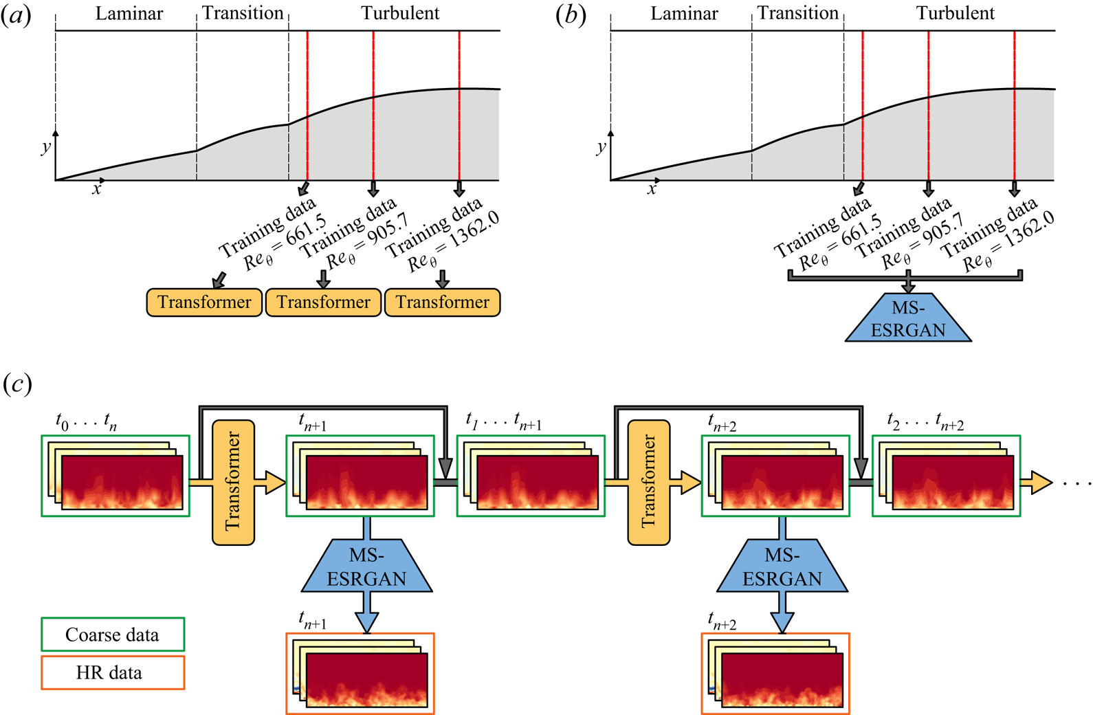
Figure 1. Schematic of (a) training procedure for the transformer, (b) training procedure for the MS-ESRGAN and (c) turbulent inflow generation using the proposed DLM.
In this study, the open-source library TensorFlow 2.4.0 (Abadi et al. Reference Abadi2016) is used for the implementation of the presented model. The source code of the model is available at https://fluids.pusan.ac.kr/fluids/65416/subview.do.
2.1. Transformer
A LSTM (Hochreiter & Schmidhuber Reference Hochreiter and Schmidhuber1997) is an artificial neural network that can handle sequential data and time-series modelling. A LSTM is a type of RNN (Rumelhart, Hinton & Williams Reference Rumelhart, Hinton and Williams1986). It has also played an essential role in modelling the temporal evolution of turbulence in various problems (Srinivasan et al. Reference Srinivasan, Guastoni, Azizpour, Schlatter and Vinuesa2019; Kim & Lee Reference Kim and Lee2020; Eivazi et al. Reference Eivazi, Guastoni, Schlatter, Azizpour and Vinuesa2021; Nakamura et al. Reference Nakamura, Fukami, Hasegawa, Nabae and Fukagata2021; Yousif & Lim Reference Yousif and Lim2022). Although LSTM is designed to overcome most of the traditional RNN limitations, such as vanishing gradients and explosion of gradients (Graves Reference Graves2012), it is usually slow in terms of training due to its architecture, which requires that the time-series data be introduced to the network sequentially. This prevents parallelisation of the training process, which is why a GPU is used in deep learning calculations. Furthermore, LSTM has shown a limitation in dealing with long-range dependencies.
The transformer (Vaswani et al. Reference Vaswani, Shazeer, Parmar, Uszkoreit, Jones, Gomez, Kaiser and Polosukhin2017) was introduced to deal with these limitations by applying the self-attention concept to compute the representations of its input and output data without feeding the data sequentially. In this study, a transformer is used to model the temporal evolution of the velocity fields that represent the turbulent inflow data.
Figure 2 shows the architecture of the transformer used in this study. Similar to the original transformer proposed by Vaswani et al. (Reference Vaswani, Shazeer, Parmar, Uszkoreit, Jones, Gomez, Kaiser and Polosukhin2017), it has two main components: encoder and decoder. The inputs of both components are passed through a positional encoder using sine and cosine functions, which can encode the order information of the input data into a vector and add it directly to the input vector. The encoder consists of six stacked encoder layers. Each layer contains a multihead self-attention sublayer and a feed-forward sublayer. The input of the multihead self-attention sublayer consists of queries ( $\boldsymbol{Q}$), keys ( $\boldsymbol{K}$) and values ( $\boldsymbol{V}$). Note that attention is a function that can map a query and set of key-value pairs to output, where the queries, keys, values and output are all vectors. The output can be calculated as the weighted sum of the values. The attention function is represented by scaled dot-product attention, which is an attention mechanism where the dot products are scaled down by $\sqrt {d_k }$. In addition, $d_k$ is the dimension of $\boldsymbol{Q}$, $\boldsymbol{K}$ and it is equal to the dimension of $\boldsymbol{V}$, i.e. $d_v$.
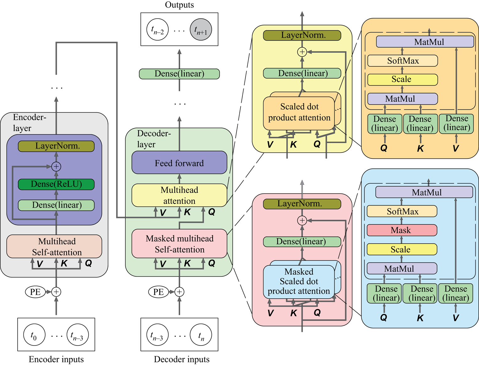
Figure 2. Architecture of the transformer. The dashed line box represents the scaled dot-product attention.
The scaled dot-product attention is calculated simultaneously for  $\boldsymbol{Q}$, $\boldsymbol{K}, \boldsymbol{V}$ by packing them into the matrices $\boldsymbol{\mathsf{Q}}, \boldsymbol{\mathsf{K}}, \boldsymbol{\mathsf{V}}$:
 \begin{equation} \mathrm{Attention}~(\boldsymbol{\mathsf{Q}}, \boldsymbol{\mathsf{K}}, \boldsymbol{\mathsf{V}}) = \mathrm{softmax} \left( \frac{\boldsymbol{\mathsf{QK}}^{\boldsymbol{\mathsf{T}}}}{\sqrt{d_k}} \right) \boldsymbol{\mathsf{V}} , \end{equation}
where softmax is a function that takes an input vector and normalises it to a probability distribution so that the output vector has values that sum to 1 (Goodfellow et al. Reference Goodfellow, Pouget-Abadie, Mirza, Xu, Warde-Farley, Ozair, Courville and Bengio2014). In the multihead self-attention sublayer,  $d_v = d_{model}/h$, where $d_{model}$ and $h$ are the dimension of the input data to the model and number of heads, respectively.
The multihead attention allows the model to jointly attend to information from different representation subspaces at different positions such that
 \begin{gather} \text{Multihead}~(\boldsymbol{\mathsf{Q}}, \boldsymbol{\mathsf{K}}, \boldsymbol{\mathsf{V}}) = \text{Concat} \left( head_1 ,\ldots, head_h \right) \boldsymbol{\mathsf{W}}^{\boldsymbol{\mathsf{o}}}, \end{gather}
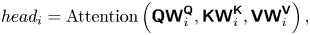 \begin{gather}head_i = \mathrm{Attention} \left( \boldsymbol{\mathsf{QW}}_i^{\boldsymbol{\mathsf{Q}}} , \boldsymbol{\mathsf{KW}}_i^{\boldsymbol{\mathsf{K}}} , \boldsymbol{\mathsf{VW}}_i^{\boldsymbol{\mathsf{V}}} \right), \end{gather}
where  $\boldsymbol{\mathsf{W}}_i^{\boldsymbol{\mathsf{Q}}}$, $\boldsymbol{\mathsf{W}}_i^{\boldsymbol{\mathsf{K}}}$ and $\boldsymbol{\mathsf{W}}_i^{\boldsymbol{\mathsf{V}}}$ are the weights corresponding to $\boldsymbol{\mathsf{Q}}$, $\boldsymbol{\mathsf{K}}$, $\boldsymbol{\mathsf{V}}$ at every head, respectively; $\boldsymbol{\mathsf{W}}^{\boldsymbol{\mathsf{o}}}$ represents the weights of the concatenated heads. $\boldsymbol{\mathsf{W}}_i^{\boldsymbol{\mathsf{Q}}} \in \mathbb {R}^{d_{model} \times d_k }$, $\boldsymbol{\mathsf{W}}_i^{\boldsymbol{\mathsf{K}}} \in \mathbb {R}^{d_{model} \times d_k }$, $\boldsymbol{\mathsf{W}}_i^{\boldsymbol{\mathsf{V}}} \in \mathbb {R}^{d_{model} \times d_v }$ and $\boldsymbol{\mathsf{W}}^{\boldsymbol{\mathsf{o}}} \in \mathbb {R}^{ hd_v \times d_{model} }$.
The multihead self-attention sublayer contains six heads of scaled dot-product attention. A residual connection (He et al. Reference He, Zhang, Ren and Sun2016) is applied around the multihead attention, followed by layer normalisation (Ba, Kiros & Hinton Reference Ba, Kiros and Hinton2016).
The second part of the encoder layer, i.e. the feed-forward sublayer, contains two dense layers with linear and rectified linear unit (ReLU) activation functions. This layer projects the vector to a larger space, where it is easier to extract the required information and then projects it back to the original space. As in the multihead self-attention sublayer, a residual connection is employed before applying layer normalisation.
Similar to the encoder, the decoder contains six decoder layers. In addition to the multihead self-attention and feed-forward sublayers, the decoder layer has a third sublayer that performs multihead attention over the output of the encoder stack. Furthermore, the multihead self-attention sublayer is changed to a masked multihead self-attention sublayer, as shown in figure 2, which is similar to the multihead self-attention sublayer with the difference that the scaled dot-product attention is changed to a masked scaled dot-product attention (Vaswani et al. Reference Vaswani, Shazeer, Parmar, Uszkoreit, Jones, Gomez, Kaiser and Polosukhin2017). The masking operation ensures that the prediction can only depend on the known outputs, a fact that prevents later information leakage. In this study, the dropout technique is applied to every sublayer before the residual connection and the rate of dropout is set to 0.1.
The square of the  $L_2$ norm error is chosen as a loss function for the transformer such that
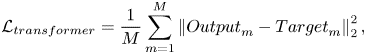 \begin{equation} \mathcal{L}_{transformer}= \frac{1}{M} \sum_{m=1}^M \left\| {Output}_m - {Target}_m \right\|_2^2, \end{equation}
where  $Output$ and $Target$ represent the output from the transformer and ground truth data, respectively, at a specific time step, $m$. Here $M$ represents the size of the training mini-batch, which is set to 64. The adaptive moment estimation (Adam) optimisation algorithm (Kingma & Ba Reference Kingma and Ba2017) is used to update the weights of the model.
2.2. MS-ESRGAN
Generative adversarial networks (Goodfellow et al. Reference Goodfellow, Pouget-Abadie, Mirza, Xu, Warde-Farley, Ozair, Courville and Bengio2014) have shown great success in image transformation and super-resolution problems (Mirza & Osindero Reference Mirza and Osindero2014; Ledig et al. Reference Ledig, Theis, Huszar, Caballero, Cunningham, Acosta, Aitken, Tejani, Totz and Shi2017; Zhu et al. Reference Zhu, Park, Isola and Efros2017; Wang et al. Reference Wang, Yu, Wu, Gu, Liu, Dong, Loy, Qiao and Tang2018). Generative adversarial network-based models have also shown promising results in reconstructing HR turbulent flow fields from coarse data (Fukami et al. Reference Fukami, Fukagata and Taira2019a; Fukami, Fukagata & Taira Reference Fukami, Fukagata and Taira2021; Güemes et al. Reference Güemes, Discetti, Ianiro, Sirmacek, Azizpour and Vinuesa2021; Kim et al. Reference Kim, Kim, Won and Lee2021; Yousif et al. Reference Yousif, Yu and Lim2021, Reference Yousif, Yu and Lim2022b; Yu et al. Reference Yu, Yousif, Zhang, Hoyas, Vinuesa and Lim2022). In a GAN model that is used for image generation, two adversarial neural networks called the generator ( $G$) and the discriminator ( $D$) compete with each other. The $G$ tries to generate artificial images with the same statistical properties as those of the real ones, whereas $D$ tries to distinguish the artificial images from the real ones. After successful training, $G$ should be able to generate artificial images that are difficult to distinguish by $D$. This process can be expressed as a min–max two-player game with a value function $V(D, G)$ such that
 \begin{equation} \substack{min\\G} ~\substack{max\\D} ~V(D,G) = \mathbb{E}_{\boldsymbol{\chi}_r \sim P_{data}(\boldsymbol{\chi}_r)} [ \log D(\boldsymbol{\chi}_r )] + \mathbb{E}_{\boldsymbol{\xi} \sim P_{\boldsymbol{\xi}}(\boldsymbol{\xi}) } [ \log (1-D(G(\boldsymbol{\xi})))], \end{equation}
where  $\boldsymbol{\chi} _r$ is the image from the ground truth data (real image) and $P_{data}(\boldsymbol{\chi} _r )$ is the real image distribution. Here $\mathbb {E}$ represents the operation of calculating the average of all the data in the training mini-batch. In the second right-hand term of (2.5), $\boldsymbol{\xi}$ is a random vector used as an input to $G$ and $D(\boldsymbol{\chi} _r)$ represents the probability that the image is real and not generated by the generator. The output from $G$, i.e. $G(\boldsymbol{\xi} )$, is expected to generate an image that is similar to the real one, such that the value of $D(G(\boldsymbol{\xi} ))$ is close to 1. Meanwhile, $D(\boldsymbol{\chi} _r)$ returns a value close to 1, whereas $D(G(\boldsymbol{\xi} ))$ returns a value close to 0. Thus, in the training process, $G$ is trained in a direction that minimises $V(D,G)$, whereas $D$ is trained in a direction that maximises $V(D,G)$.
In this study, MS-ESRGAN (Yousif et al. Reference Yousif, Yu and Lim2021) is used to perform super-resolution reconstruction of the velocity fields predicted by the transformer. The MS-ESRGAN is based on the enhanced super-resolution GAN (ESRGAN) (Wang et al. Reference Wang, Yu, Wu, Gu, Liu, Dong, Loy, Qiao and Tang2018). Figure 3 shows the architecture of MS-ESRGAN. As shown in figure 3(a),  $G$ consists of a deep CNN represented by residual in residual dense blocks (RRDBs) and multiscale parts (MSP). Note that the input to $G$ is low-resolution data, which are first passed through a convolutional layer and then through a series of RRDBs. The MSP, consisting of three parallel convolutional submodels with different kernel sizes, is applied to the data features extracted by RRDBs. More details for MSP can be found in Yousif et al. (Reference Yousif, Yu and Lim2021, Reference Yousif, Yu and Lim2022b). The outputs of the three submodels are summed and passed through a final convolutional layer to generate HR artificial data $(\boldsymbol{\chi} _a)$. Figure 3(b) shows that the artificial and real data are fed to $D$ and passed through a series of convolutional, batch normalisation and leaky ReLU layers. As a final step, the data are crossed over a convolutional layer. The non-transformed discriminator outputs using the real and artificial data, i.e. $C(\boldsymbol{\chi} _r )$ and $C(\boldsymbol{\chi} _a )$, are used to calculate the relativistic average discriminator value $D_{Ra}$ (Jolicoeur-Martineau Reference Jolicoeur-Martineau2018):
 \begin{gather} D_{Ra} (\boldsymbol{\chi}_r , \boldsymbol{\chi}_a ) = \sigma (C \left(\boldsymbol{\chi}_r ) \right) - \mathbb{E}_{\boldsymbol{\chi}_a} \left[C ( \boldsymbol{\chi}_a) \right], \end{gather}
 \begin{gather}D_{Ra} (\boldsymbol{\chi}_a , \boldsymbol{\chi}_r ) = \sigma (C \left(\boldsymbol{\chi}_a) \right) - \mathbb{E}_{\boldsymbol{\chi}_r} \left[C ( \boldsymbol{\chi}_r) \right], \end{gather}
where  $\sigma$ is the sigmoid function. In (2.6) and (2.7), $D_{Ra}$ represents the probability that the output from $D$ using the real image is relatively more realistic than the output using the artificial image.
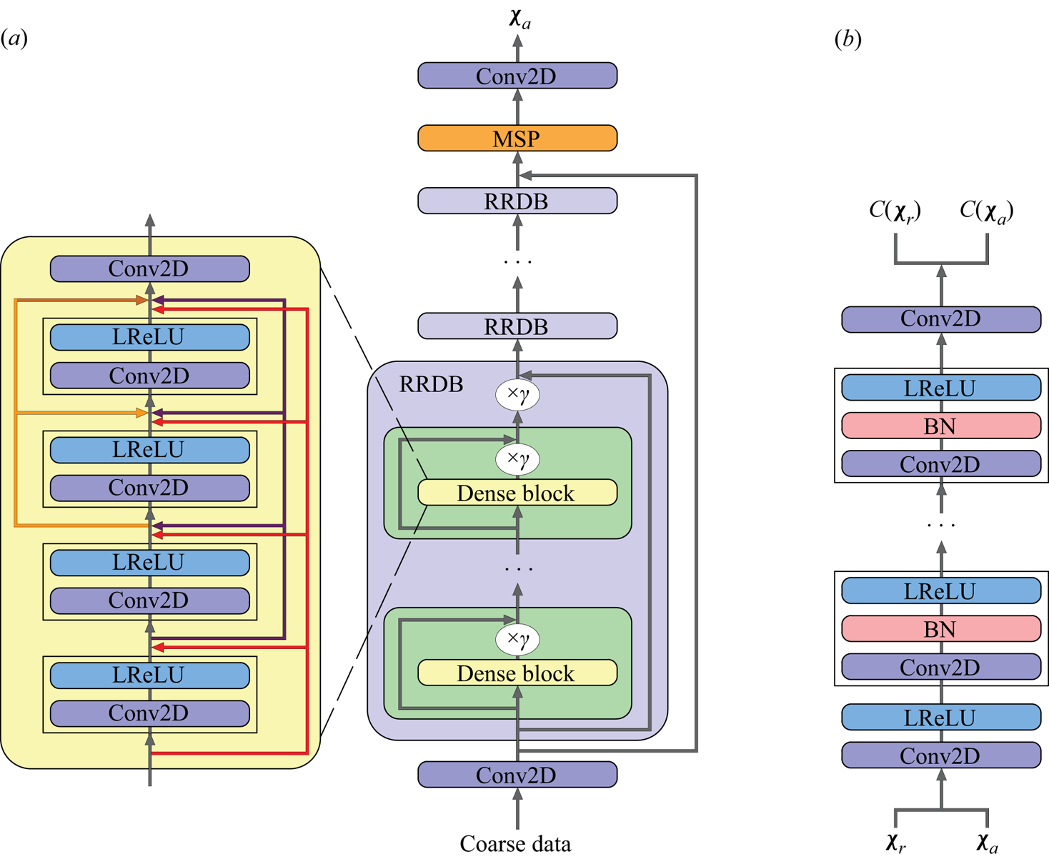
Figure 3. Architecture of MS-ESRGAN. (a) The generator, where  $\gamma$ is the residual scaling parameter which is set to 0.2 in this study, and (b) the discriminator.
Then, the discriminator loss function is defined as follows:
 \begin{equation} \ell_D^{Ra} ={-}\mathbb{E}_{\boldsymbol{\chi}_r} \left[ \log (D_{Ra} (\boldsymbol{\chi}_r , \boldsymbol{\chi}_a)) \right] - \mathbb{E}_{\boldsymbol{\chi}_a} \left[ \log (1 - D_{Ra} (\boldsymbol{\chi}_a, \boldsymbol{\chi}_r )) \right]. \end{equation}
The adversarial loss function of the generator can be expressed in a symmetrical form as follows:
 \begin{equation} \ell_G^{Ra} ={-}\mathbb{E}_{\boldsymbol{\chi}_r} \left[ \log (1 - D_{Ra} (\boldsymbol{\chi}_r , \boldsymbol{\chi}_a )) \right] - \mathbb{E}_{\boldsymbol{\chi}_a} \left[ \log (D_{Ra} (\boldsymbol{\chi}_a , \boldsymbol{\chi}_r )) \right]. \end{equation}
The total loss function of the generator is defined as
 \begin{equation} \mathcal{L}_G = \ell_G^{Ra} + \beta \ell_{pixel} + \ell_{perceptual}, \end{equation}
where  $\ell _{pixel}$ is the error calculated based on the pixel difference of the generated and ground truth data; $\ell _{perceptual}$ represents the difference between features that are extracted from the real and the artificial data. The pretrained CNN VGG-19 (Simonyan & Zisserman Reference Simonyan and Zisserman2014) is used to extract the features using the output of three different layers (Yousif et al. Reference Yousif, Yu and Lim2021). Here, $\beta$ is a weight coefficient and its value is set to be 5000. The square of the $L_2$ norm error is used to calculate $\ell _{pixel}$ and $\ell _{perceptual}$. The size of the mini-batch is set to 32. As in the transformer model, the Adam optimisation algorithm is used to update the weights of the model.
3. Data description and preprocessing
The transitional boundary layer database (Lee & Zaki Reference Lee and Zaki2018) available at the Johns Hopkins turbulence databases (JHTDB) is considered in this study for the training and testing of the DLM. The database was obtained via DNS of incompressible flow over a flat plate with an elliptical leading edge. In the simulation, the half-thickness of the plate  $L$ and the free stream velocity $U_\infty$ are used as a reference length and velocity. In addition, $x$,
$x$,  $y$ and $z$ are defined as the streamwise, wall-normal and spanwise coordinates, respectively, with the corresponding velocity components $u$,
$u$,  $v$ and $w$. Note that the same definitions of the coordinates and velocity components are used in this study.
In the simulation, the length of the plate,  $L_x = 1050L$ measured from the leading edge ( $x$ = 0), the domain height, $L_y = 40L$ and the width of the plate, $L_z = 240L$. The stored database in JHTDB is in the range $x \in [30.2185, 1000.065]L$, $y \in [0.0036, 26.488 ]L$ and $z \in [ 0, 240]L$. The corresponding number of grid points is $N_x \times N_y \times N_z = 3320 \times 224 \times 2048 \approx 1.5 \times 10^9$. The database time step is $\Delta t = 0.25L/U_\infty$. The stored database spans the following range in momentum-thickness-based Reynolds number, $Re_\theta = U_\infty \theta /\nu \in [105.5,1502.0 ]$, where $\theta$ represents the momentum thickness and $\nu$ is the kinematic viscosity. More details for the simulation and database can be found in Lee & Zaki (Reference Lee and Zaki2018) and on the website of JHTDB.
In this study, the datasets within the range of  $Re_\theta \in [ 661.5, 1502.0 ]$ are considered for training and testing the DLM. This range of $Re_\theta$ in the database represents the fully turbulent part of the flow (Lee & Zaki Reference Lee and Zaki2018). Datasets of the velocity components are collected from various $y$–
$y$– $z$ planes along the streamwise direction, with a number of ${\rm snapshots} = 4700$ for every plane. To reduce the computational cost, the original size of each plane, $N_y \times N_z = 224 \times 2048$ is reduced to $112 \times 1024$. Furthermore, to increase the amount of training and testing data, every selected plane is divided into four identical sections ( $y$–
$y$– $z$ planes) along the spanwise direction, resulting in $N_y \times N_z = 112 \times 256$ for each section. To obtain the coarse data, the size of the data is further reduced to $N_y \times N_z = 14 \times 32$, which is obtained by selecting distributed points in the fields. The distribution of the points is obtained in a stretching manner such that more points can be selected near the wall. A time series of 4000 snapshots for each section are used to train the DLM, resulting in a total number of training ${\rm snapshots} = 4000\times 4\times 3=48\,000$. The fluctuations of the velocity fields are used in the training and prediction processes. The input data to the DLM are normalised using the min–max normalisation function to produce values between 0 and 1.
4. Results and discussion
4.1. Results from the DLM trained at various  $Re_\theta$

This section examines the capability of the proposed DLM to generate turbulent inflow data at three different Reynolds numbers for which the network has already been trained,  $Re_\theta = 661.5$, 905.7 and 1362.0. Figures 4–6 show the instantaneous streamwise velocity ( $u^+$) and vorticity ( $\omega _x^+$) fields of the DNS and the predicted data for three different time steps, where the superscript ‘ $+$’ denotes normalisation by viscous inner scale; in the figures, $\delta$ represents the boundary layer thickness. The figures show that the instantaneous flow fields can be predicted using the model with a commendable agreement with the DNS data. Note that the model has shown a capacity to predict the instantaneous flow fields for a long period of time, more than the one required for the flow data to reach a statistically stationary state (reaching fixed first and second-order statistics over time), i.e. for a number of time $\text {steps} = 10\,000$.
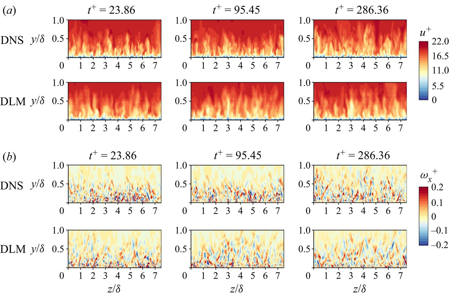
Figure 4. Instantaneous streamwise (a) velocity and (b) vorticity fields at  $Re_\theta = 661.5$, for three different instants. Reference (DNS) and predicted (DLM) data are shown.

Figure 5. Instantaneous streamwise (a) velocity and (b) vorticity fields at  $Re_\theta = 905.7$, for three different instants. Reference (DNS) and predicted (DLM) data are shown.
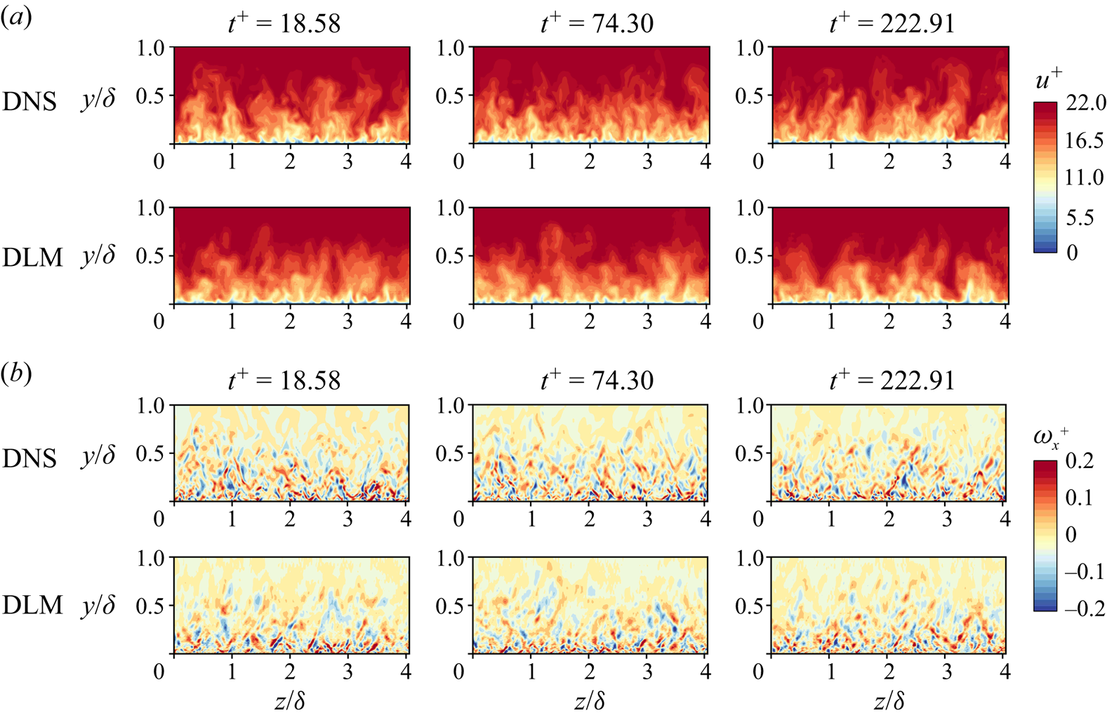
Figure 6. Instantaneous streamwise (a) velocity and (b) vorticity fields at  $Re_\theta = 1362.0$, for three different instants. Reference (DNS) and predicted (DLM) data are shown.
The shape factor (ratio of displacement to momentum thickness of the TBL) values of the DNS and predicted velocity fields are shown in table 1. A slight under-prediction can be seen in all the predicted values with the highest deviation of 2.95 % at  $Re_\theta = 661.5$.
Table 1. Shape factor values of the reference (DNS) and predicted (DLM) data.
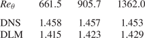
Figure 7 shows the probability density functions (p.d.f.s) of the velocity components ( $u^+$, $v^+$ and $w^+$) plotted against the wall-normal distance ( $y^+$). The figure reveals that the p.d.f. plots of the generated velocity components are in agreement with the p.d.f. plots obtained from the DNS data, indicating the capability of the model in predicting the velocity fields with distributions of the velocity components that are consistent with those of the DNS data.

Figure 7. Probability density functions of the velocity components as a function of the wall-normal distance. The shaded contours represent the results from the DNS data and the dashed ones represent the results from the predicted data. The contour levels are in the range of 20 %–80 % of the maximum p.d.f. with an increment of 20 %: (a–c)  $Re_\theta = 661.5$; (d–f) $Re_\theta = 905.7$; (g–i) $Re_\theta = 1362.0$.
Figures 8–10 compare the turbulence statistics of the generated velocity fields with the turbulence statistics of the DNS data. As shown in the figures, the mean streamwise velocity profile ( $U^+$) for all the three Reynolds numbers shows excellent agreement with the results obtained from the DNS. The comparison of root mean square (r.m.s.) profiles of the velocity components ( $u_{rms}^+$, $v_{rms}^+$ and $w_{rms}^+$) reveals good agreement with the DNS results. However, the profile of the Reynolds shear stress ( $\overline {u'v'}^+$) shows a slight under-prediction in the region between near the wall and the maximum Reynolds shear stress, and the profile values in this region improve as the Reynolds number increases. This might be attributed to the fact that with the increase in the boundary-layer thickness, the effect of zero padding in the convolution processes is decreased in MS-ESRGAN, resulting in a better prediction of the velocity fields in this region of the boundary layer. These results are consistent with the results from table 1.
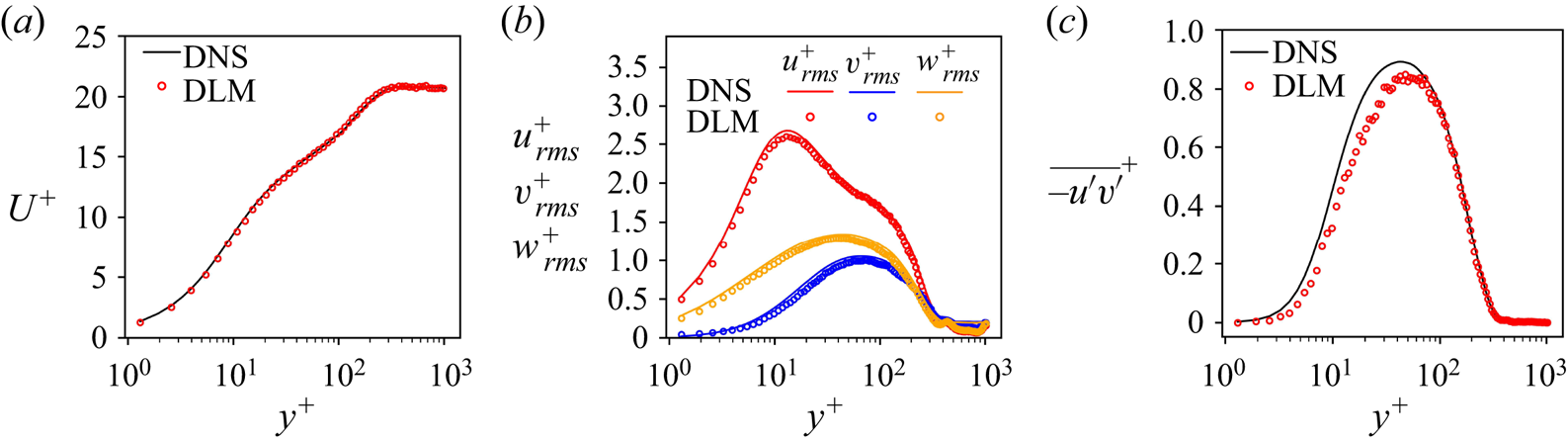
Figure 8. Turbulence statistics of the flow at  $Re_\theta = 661.5$: (a) mean streamwise velocity profile; (b) r.m.s. profiles of the velocity components; (c) Reynolds shear stress profile.

Figure 9. Turbulence statistics of the flow at  $Re_\theta = 905.7$: (a) mean streamwise velocity profile; (b) r.m.s. profiles of the velocity components; (c) Reynolds shear stress profile.

Figure 10. Turbulence statistics of the flow at  $Re_\theta = 1362.0$: (a) mean streamwise velocity profile; (b) r.m.s. profiles of the velocity components; (c) Reynolds shear stress profile.
The capability of the proposed DLM to produce realistic spatial spectra of the velocity fields is investigated by employing the premultiplied spanwise wavenumber spectrum,  $k_z \varPhi _{\alpha \alpha }$, where $\varPhi _{\alpha \alpha }$ represents the spanwise wavenumber spectrum, $\alpha$ represents the velocity component and $k_z$ is the spanwise wavenumber. Figure 11 shows the contour plots of $k_z^+ \varPhi _{\alpha \alpha }^+$ as a function of $y^+$ and the spanwise wavelength, $\lambda _z^+$. The figure shows that the spectra of the velocity components are generally consistent with those obtained from the DNS data with a slight deviation at the high wavenumbers. This indicates that the two-point correlations of the generated velocity components are consistent with those obtained from the DNS data, further supporting the excellent performance of the proposed DLM to properly represent the spatial distribution of the velocity fields. It is worth noting that the ability of the model to reproduce accurate spectra is essential in generating the turbulent inflow conditions to guarantee that the turbulence will be sustained after introducing the synthetic-inflow conditions; otherwise, the generated inflow would require very long distances to reach ‘well-behaved’ turbulent conditions, and these fluctuations could also dissipate.

Figure 11. Premultiplied spanwise wavenumber energy spectra of the velocity components as a function of the wall-normal distance and the spanwise wavelength. The shaded contours represent the results from the DNS data and the dashed ones represent the results from the predicted data. The contour levels are in the range of 10 %–90 % of the maximum  $k_z^+ \varPhi _{\alpha \alpha }^+$ with an increment of 10 %: (a–c) $Re_\theta = 661.5$; (d–f) $Re_\theta = 905.7$; (g–i) $Re_\theta = 1362.0$.
To evaluate the performance of the proposed DLM to generate the velocity fields with accurate dynamics, the frequency spectrum,  $\phi _{\alpha \alpha }^+$, as a function of $y^+$ and the frequency, $f^+$ is represented in figure 12. Note that the spectra obtained from the generated velocity fields show a commendable agreement with those of the DNS data, indicating that the proposed DLM can produce turbulent inflow conditions with a temporal evolution of the velocity fields that is consistent with that of the DNS.

Figure 12. Frequency spectra of the velocity components as a function of the wall-normal distance and the frequency. The shaded contours represent the results from the DNS data and the dashed ones represent the results from the predicted data. The contour levels are in the range of 10 %–90 % of the maximum  $\phi _{\alpha \alpha }^+$ with an increment of 10 %: (a–c) $Re_\theta = 661.5$; (d–f) $Re_\theta = 905.7$; (g–i) $Re_\theta = 1362.0$.
4.2. Interpolation and extrapolation capability of the DLM
This section investigates the performance of the proposed DLM to generate turbulent inflow conditions at Reynolds numbers that are not used in the training process. The velocity fields at  $Re_\theta = 763.8$ and 1155.1 are used as examples of the velocity fields that fall between the Reynolds numbers used in the training process, i.e. the interpolation ability of the model is investigated using the flow fields at these Reynolds numbers.
Figure 13 shows the instantaneous streamwise velocity and vorticity fields for the flow at  $Re_\theta = 763.8$. It is worth noting that the transformer trained for the flow at the nearest $Re_\theta$, i.e. $Re_\theta = 661.5$ is used to predict the temporal evolution of the velocity fields. The figure shows that the main features of the flow fields can be obtained with relatively good precision; however, the details of the predicted velocity fluctuations are not clearly shown. Similar results can be observed in figure 14 for the predicted velocity fields at $Re_\theta = 1155.1$. Here, the current transformers trained for the flow at $Re_\theta = 905.7$ and 1362.0 are used to predict the temporal evolution of the velocity fields.

Figure 13. Instantaneous streamwise (a) velocity and (b) vorticity fields at  $Re_\theta = 763.8$, for three different instants. Reference (DNS) and predicted (DLM) data are shown.

Figure 14. Instantaneous streamwise (a) velocity and (b) vorticity fields at  $Re_\theta = 1155.1$, for three different instants. Cases 1 and 2 represent the prediction using the transformer that is trained for the flow at $Re_\theta = 905.7$ and 1362.0, respectively.
The turbulence statistics of the flow at  $Re_\theta = 763.8$ and 1155.1 are shown in figures 15 and 16, respectively. Although the mean streamwise velocity and the r.m.s. profiles of the spanwise and wall-normal velocity components show an ability of the DLM to predict reasonably well, the r.m.s. profile of the streamwise velocity component and the Reynolds shear stress show an under-prediction due to the lack of detailed information on the velocity fluctuations.

Figure 15. Turbulence statistics of the flow at  $Re_\theta = 763.8$: (a) mean streamwise velocity profile; (b) r.m.s. profiles of the velocity components; (c) Reynolds shear stress profile.

Figure 16. Turbulence statistics of the flow at  $Re_\theta = 1155.1$. Cases 1 and 2 represent the prediction using the transformer model trained for the flow at $Re_\theta = 905.7$ and 1362.0, respectively. (a) Mean streamwise velocity profile; (b) r.m.s. profiles of the velocity components; (c) Reynolds shear stress profile.
The extrapolation ability of the DLM is evaluated using the flow fields at  $Re_\theta = 1502.0$, which is higher than the maximum $Re_\theta$ used to train the transformer and MS-ESRGAN, i.e. $Re_\theta = 1362.0$. The transformer trained for the flow at $Re_\theta = 1362.0$ is used to predict the dynamics of the velocity fields. Figure 17 shows that the generated instantaneous streamwise velocity and vorticity fields generally have similar accuracy to the interpolated flow fields. Meanwhile, the turbulence statistics show a deviation from the DNS statistics, as shown in figure 18. This can be attributed to the lack of details of the velocity fluctuations and the extrapolation process that relies on the flow information at one Reynolds number compared with the interpolation process where the flow falls within the range of the Reynolds numbers that the MS-ESRGAN is trained for.

Figure 17. Instantaneous streamwise (a) velocity and (b) vorticity fields at  $Re_\theta = 1502.0$ for three different instants. Reference (DNS) and predicted (DLM) data are shown.

Figure 18. Turbulence statistics of the flow at  $Re_\theta = 1502.0$. (a) mean streamwise velocity profile; (b) r.m.s. profiles of the velocity components; (c) Reynolds shear stress profile.
Finally, the accuracy of the spectral content of the interpolated and extrapolated velocity components is examined in figure 19 by employing the premultiplied spanwise wavenumber spectrum. These results indicate that the spectra are produced with relatively good accuracy for the low–moderate wavenumbers.

Figure 19. Premultiplied spanwise wavenumber energy spectra of the velocity components as a function of the wall distance and wavelength. The shaded contours represent the results from the DNS data; the dashed-black contours represent the results from the predicted velocity data at  $Re_\theta = 763.8$ and 1502.0; the dashed-brown and grey contours represent the results from the velocity data at $Re_\theta = 1155.1$ predicted using the transformer model trained for the flow at $Re_\theta = 905.7$ and 1362.0, respectively. The contour levels are in the range of 10 %–90 % of the maximum $k_z^+ \varPhi _{\alpha \alpha }^+$ with an increment of 10 %: (a–c) $Re_\theta = 763.8$; (d–f) $Re_\theta =1155.1$; (g–i) $Re_\theta =1502.0$.
4.3. Error analysis, transfer learning and computational cost
The performance of the proposed DLM is further statistically investigated using the  $L_2$ norm error of the predicted data for all the Reynolds numbers used in this study,
 \begin{equation} \varepsilon = \frac{1}{J} \sum_{j=1}^J \frac{\left\| {\alpha}_j^{\mathrm{DNS}} - {\alpha}_j^{\mathrm {DLM}}\right\|_2 }{\left\| {\alpha}_j^{\mathrm {DNS}}\right\|_2}, \end{equation}
where  $\alpha _j^{\mathrm {DNS}}$ and $\alpha _j^{\mathrm {DLM}}$ represent the ground truth (DNS) and the predicted velocity components using the DLM, respectively, and $J$ represents the number of the test snapshots.
Figure 20 shows that as the Reynolds number increases, no significant differences can be seen in the error values of the predicted velocity fields. However, as expected, the error shows higher values for the interpolated and extrapolated velocity fields compared with the error of the predicted velocity fields at the Reynolds numbers that the DLM is trained for. Additionally, in contrast with the aforementioned statistical results, the error values are relatively high for the wall-normal and spanwise velocity fields. This indicates that the DLM has learned to model the structure of the flow with generally accurate turbulence statistics and spatiotemporal correlations, rather than reproducing the time sequence of the flow data. This observation is consistent with the results obtained by Fukami et al. (Reference Fukami, Nabae, Kawai and Fukagata2019b), Kim & Lee (Reference Kim and Lee2020) and Yousif et al. (Reference Yousif, Yu and Lim2022a). Furthermore, using input data of size  $7\times 16$ in the training of the DLM shows a slight reduction in the model performance, indicating the capability of the DLM to generate the turbulent inflow data even if it is trained with extremely coarse input data.

Figure 20. The  $L_2$ norm error of the predicted velocity fields: (a) streamwise velocity; (b) wall-normal velocity; (c) spanwise velocity. Cases 1 and 2 represent the results from the velocity data at $Re_\theta = 1155.1$ predicted using the transformer model trained for the flow at $Re_\theta = 905.7$ and 1362.0, respectively.
It is worth mentioning that the transfer learning (TL) technique is used in this study (Guastoni et al. Reference Guastoni, Guemes, Ianiro, Discetti, Schlatter, Azizpour and Vinuesa2021; Yousif et al. Reference Yousif, Yu and Lim2021, Reference Yousif, Yu and Lim2022a). The weights of the transformer are sequentially transferred for every training  $y$–
$y$– $z$ plane in the flow. First, the transformer is trained for the flow at the lowest Reynolds number, i.e. $Re_\theta = 661.5$. After that, the weights of the model are transferred for the training using the next $Re_\theta$ data and so on. The results from using TL in this study show that with the use of only 25 % of the training data for the transformer model, the computational cost (represented by the training time) can be reduced by 52 % without affecting the prediction accuracy. These results are consistent with the results obtained by Guastoni et al. (Reference Guastoni, Guemes, Ianiro, Discetti, Schlatter, Azizpour and Vinuesa2021) and Yousif et al. (Reference Yousif, Yu and Lim2021, Reference Yousif, Yu and Lim2022a).
The total number of trainable parameters of the DLM is  $356.5 \times 10^6$ ( $305.5 \times 10^6$ for the transformer and $51 \times 10^6$ for the MS-ESRGAN). The training of the transformer model for all the three Reynolds numbers used in this study using a single NVIDIA TITAN RTX GPU with the aid of TL requires approximately 23 hours. Meanwhile, the training of the MS-ESRGAN requires approximately 32 hours. Thus, the total training time of the DLM model is 55 hours, indicating that the computational cost of the model is relatively lower than the cost of the DNS that is required to generate the velocity fields. Furthermore, this computational cost is required only once, i.e. for the training of the model. Since the prediction process is computationally inexpensive and does not need any data for the prediction (except the initial instantaneous fields), the DLM can also be considered efficient in terms of storing and transferring the inflow data.
4.4. Simulation of spatially developing TBL using the turbulent inflow data
In order to examine the feasibility of applying the DLM-based turbulent inflow conditions, the generated data are utilised to perform an inflow–outflow large-eddy simulation (LES) of flat plate TBL spanning  $Re_\theta = 1362\unicode{x2013}1820$. The open-source computational fluid dynamics finite-volume code OpenFOAM-5.0x is used to perform the simulation. The dimensions of the computational domain are 20 $\delta _0$, 1.8 $\delta _0$ and 4 $\delta _0$ in the streamwise, wall-normal and spanwise directions, respectively, where $\delta _0$ represents the boundary layer thickness at the inlet section of the domain. The corresponding grid ${\rm size} = 320 \times 90 \times 150$. The grid points have a uniform distribution in the streamwise and spanwise directions while local grid refinement is applied near the wall using the stretching grid technique in the wall-normal direction. The spatial spacing at the midpoint of the domain is $\Delta x^+ \approx 15.4$, $\Delta y^+_{wall} \approx 0.2$ and $\Delta z^+ \approx 6.5$, where $y^+ _{wall}$ represents the spatial spacing in the wall-normal direction near the wall. A no-slip boundary condition is applied to the wall, while periodic boundary conditions are applied to the spanwise direction. A slip boundary condition is assigned to the top of the domain, whereas an advection boundary condition is applied to the outlet of the domain. The pressure implicit split operator algorithm is employed to solve the coupled pressure momentum system. The dynamic Smagorinsky model (Germano et al. Reference Germano, Piomelli, Moin and Cabot1991) is applied for the subgrid-scale modelling. All the discretisation schemes used in the simulation have second-order accuracy. The generated inflow data are linearly interpolated in time to have a simulation time step $\Delta t = 0.0017 \delta _0/U_\infty$ yielding a maximum Courant number of 0.8. The statistics from the simulation are accumulated over a period of 620 $\delta _0/U_\infty$ after an initial run with a period of 60 $\delta _0/U_\infty$ or 3 flow through.
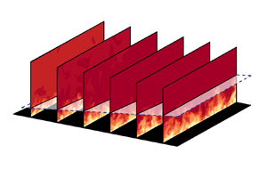
The formation of the instantaneous vortical structures of the flow is visualised by utilising the  $Q$-criterion vortex identification method (Hunt, Wray & Moin Reference Hunt, Wray and Moin1988) in figure 21. Smooth development of the coherent structures represented by the hairpin-vortex-like structures (Adrian Reference Adrian2007) can be observed from the figure with no noticeable formation of artificial turbulence at the inlet section of the domain. This indicates that the inflow data obtained from the DLM could represent most of the flow physics at the inlet section, resulting in a negligible developing distance upstream of the domain.

Figure 21. Isosurfaces of instantaneous vortical structures ( $Q$-criterion $= 0.54U_\infty ^2/\delta _0^2$) from the inflow–outflow simulation coloured by the streamwise velocity.
A comparison of the mean streamwise velocity and Reynolds shear stress profiles at  $Re_\theta = 1400$ with the DNS results are provided in figure 22. The mean streamwise velocity profile is in excellent agreement with the DNS results. Furthermore, the Reynolds shear stress profile is consistent with the DNS results in most of the boundary layer regions.

Figure 22. Turbulence statistics from the inflow–outflow simulation at  $Re_\theta = 1400$ compared with the DNS results: (a) mean streamwise velocity profile; (b) Reynolds shear stress profile.
To further evaluate the accuracy of the inflow conditions, statistics obtained from the simulation are compared with the inflow–outflow LES results of Lund et al. (Reference Lund, Wu and Squires1998) and DNS results of Spalart (Reference Spalart1988). Figure 23 shows the profiles of the mean streamwise velocity and Reynolds shear stress profiles at  $Re_\theta = 1530$. An agreement can be observed with Lund et al. (Reference Lund, Wu and Squires1998) results of the modified Spalart (recycling–rescaling) method and the results of Spalart (Reference Spalart1988) ( $Re_\theta = 1410$) in the inner region of the boundary layer, however, a deviation can be observed in the outer region. This might be attributed to the fact that the original DNS data that are used to train the DLM contain free stream turbulence (Lee & Zaki Reference Lee and Zaki2018).

Figure 23. Turbulence statistics from the inflow–outflow simulation at  $Re_\theta = 1530$ compared with the results of Lund et al. (Reference Lund, Wu and Squires1998) and Spalart (Reference Spalart1988): (a) mean streamwise velocity profile; (b) Reynolds shear stress profile.
The evolution of the shape factor  $H$ is shown in figure 24(a). Here the result from the simulation is generally consistent with the DNS and Spalart (Reference Spalart1988) results, and within $5\,\%$ of the modified Spalart method from Lund et al. (Reference Lund, Wu and Squires1998). The result of the skin-friction coefficient ( $C_f$) in figure 24(b) shows an agreement with the results from Lund et al. (Reference Lund, Wu and Squires1998) and Spalart (Reference Spalart1988) with an over-prediction of approximately $8\,\%$ compared with the DNS results. The change in the shape factor slope and the over-prediction of the skin-friction coefficient compared with the DNS result can be attributed to the numerical set-up of the inflow–outflow simulation. Note that in the work of Lund et al. (Reference Lund, Wu and Squires1998), the inflow data were generated from precursor simulations that have the same $y$–
$y$– $z$ plane size as the inlet section of the inflow-outflow simulations, and no spatial or time interpolation was applied to the inflow data.

Figure 24. Evolution of the shape factor and skin-friction coefficient in the inflow–outflow simulation compared with the results of the DNS (Lund et al. Reference Lund, Wu and Squires1998; Spalart Reference Spalart1988): (a) shape factor; (b) skin-friction coefficient.
The above results suggest that the turbulent inflow data that are generated by the proposed DLM can be practically used as inflow conditions for simulations that do not necessarily have the same spatial and time resolutions as the generated data, which is the case in the simulation described in this section.
5. Conclusions
This study proposed a deep-learning-based method to generate turbulent inflow conditions for spatially developing TBL simulations. A combination of a transformer and MS-ESRGAN was used to build the inflow generator. The transformer was trained to model the temporal evolution of the velocity fields represented by various ( $y$–
$y$– $z$) planes of spatially limited data. Meanwhile, MS-ESRGAN was trained to perform super-resolution reconstruction of the predicted velocity fields.
The generated instantaneous velocity fields showed an excellent agreement with the DNS results for the velocity fields at Reynolds numbers that the DLM was trained for. The model also successfully reproduced the turbulence statistics with commendable accuracy. Furthermore, the model reproduced the spectra of the velocity components with accurate precision, indicating accurate spatial and temporal correlations of the generated velocity components, which further supports the ability of the model to maintain the realistic behaviour of the velocity fields.
The performance of the proposed model was further examined using velocity fields at Reynolds numbers that were not used in the training process. The instantaneous and statistical results showed a reasonable accuracy for the interpolated and extrapolated velocity fields. The spectra of the velocity components revealed a relatively good agreement with the results from the actual velocity data, with a deviation that can be observed at high wavenumbers. These results suggest that the model can generate the turbulent inflow conditions for the flow at Reynolds numbers that are not necessarily used in the training of the model.
The results obtained from the error analysis showed that the increase in the Reynolds number has no significant effect on the error values of the predicted velocity fields, indicating that the model is robust to the increase of the Reynolds number. The use of TL in the training of the transformer revealed a noticeable reduction in the computational cost of the DLM without affecting the precision of the prediction.
The inflow–outflow simulation results showed the feasibility of applying the generated turbulent inflow conditions to turbulent flow simulations as a negligible developing distance upstream of the domain is required for the TBL to reach the target statistics.
This study showed for the first time that a transformer-based model could be effectively used for modelling the dynamics of turbulent flows with the ability to perform parallel computing during the training process, which is not possible in LSTM-based models. It also paves the way for utilising synthetic-inflow generators for large-scale turbulence simulations using deep learning, with significant promise in terms of computational savings.
Funding
This work was supported by the ‘Human Resources Program in Energy Technology’ of the Korea Institute of Energy Technology Evaluation and Planning (KETEP) and granted financial resources from the Ministry of Trade, Industry & Energy, Republic of Korea (no. 20214000000140). In addition, this work was supported by the National Research Foundation of Korea (NRF) with a grant funded by the Korean government (MSIP) (no. 2019R1I1A3A01058576). This work was also supported by the National Supercomputing Center with supercomputing resources including technical support (KSC-2021-CRE-0244). R.V. acknowledges the financial support from the ERC grant no. ‘2021-CoG-101043998, DEEPCONTROL’.
Declaration of interests
The authors report no conflict of interest.


 Open access