


1. Introduction
Interests in stratified Taylor–Couette flows have ranged from understanding the fundamentals of the dynamics in a realizable laboratory flow, its relevance as a canonical example of the interplay between rotation, stable density stratification, velocity shear and horizontal boundaries (all common ingredients of large-scale geophysical flows in oceans and the atmosphere), to its potential in providing insight into accretion disks (Hua, Moore & Le Gentil Reference Hua, Moore and Le Gentil1997b; Yavneh, McWilliams & Molemaker Reference Yavneh, McWilliams and Molemaker2001; Shalybkov & Rüdiger Reference Shalybkov and Rüdiger2005). Unstratified Taylor–Couette flows have been extensively studied (Tagg Reference Tagg1994; Grossmann, Lohse & Sun Reference Grossmann, Lohse and Sun2015). In comparison, the literature on stratified Taylor–Couette flows is more limited.
The richness of the dynamics of Taylor–Couette flow in part stems from the large set of governing parameters. There are three length scales characterizing the geometry: the radii of the inner and outer cylinders,  $R_i$ and $R_o$, and their height $H$; these provide two governing parameters, the radius ratio $\eta =R_i/R_o$ and the aspect ratio $\gamma =H/ {\varDelta _R}$, where $ {\varDelta _R}=R_o-R_i$ is the annular gap. The rotation rates of the cylinders and the top and bottom endwalls, in general, are independent. Typically, the inner cylinder rotation rate $\varOmega$ is used to define a Reynolds number ${\textit {Re}}=\varOmega R_i {\varDelta _R}/\nu$, where $\nu$ is the kinematic viscosity, and a ratio of outer-to-inner cylinder rotation rates, $\mu$, is introduced. Most commonly, a stationary outer cylinder is considered (with $\mu =0$), but the richness associated with $\mu \ne 0$ is extensive (Coles Reference Coles1965; Andereck, Liu & Swinney Reference Andereck, Liu and Swinney1986). The endwalls are usually either co-rotating with one of the cylinders or are both stationary. However, their differential rotation introduces a different dynamics due to the resulting global meridional circulation (Lopez, Marques & Shen Reference Lopez, Marques and Shen2004). Endwalls are often viewed as a nuisance and are often ignored in theoretical and numerical models, and various experimental strategies have been tried to mitigate their impacts on the dynamics (Burin et al. Reference Burin, Ji, Schartman, Cutler, Heitzenroeder, Liu, Morris and Raftopolous2006; Avila Reference Avila2012; Leclercq et al. Reference Leclercq, Partridge, Augier, Dalziel and Kerswell2016c). Stratification introduces additional parameters, principally the Brunt–Väisälä buoyancy frequency, $N$, and the diffusivity of the stratifying agent, $\kappa$. The ratio of the inner cylinder rotation rate and the buoyancy frequency is the Froude number, ${\textit {Fr}}=\varOmega /N$, and the ratio of the kinetic viscosity and the diffusivity is the Prandtl number ${\textit {Pr}}=\nu /\kappa$ if the stratifying agent is temperature. If stratification is due to a dissolved concentration, such as salt, this ratio is called the Schmidt number, ${\textit {Sc}}$ (although the two names are used for either case in the literature). The nature of the stratifying agent has important implications for the boundary conditions. For salt stratification, all boundaries are of zero-flux Neumann type, whereas with temperature stratification, some are zero flux and others are fixed temperature Dirichlet type.
Early theoretical considerations of stratified Taylor–Couette flow date back to Thorpe (Reference Thorpe1966), who determined from highly idealized model equations that stratification resulted in a higher critical inner cylinder rotation rate for instability with a reduced axial wavelength. The analysis only considered flows with a stationary outer cylinder, and the idealizations included restricting the linear stability analysis to only allowing axisymmetric and axially periodic modes. Withjack & Chen (Reference Withjack and Chen1974) conducted some of the first experiments in vertically stratified Taylor–Couette flows. Their annulus had a radius ratio  $\eta =0.2$, various cylinder rotation ratios and linear density gradients. With increasing density gradient, instability was inhibited, with onset occurring at larger inner cylinder rotation rates, and the mode of instability broke the axisymmetry of the basic state, resulting in rotating waves, with a cellular-like structure of significantly shorter axial extent than the Taylor cells typically found in unstratified experiments (see their figures 5 and 6). Their subsequent attempt to explain their experimental observations using linear stability analysis came up short due to various idealization used (Withjack & Chen Reference Withjack and Chen1975); in particular, their analysis was restricted to axisymmetric flow that is periodic in the axial direction. Nevertheless, the general experimental observations that the linear density gradient inhibits onset and that the axial scale of the instability cells is diminished were borne out.
In a series of experiments, linear stability analyses and nonlinear simulations, Boubnov, Gledzer & Hopfinger (Reference Boubnov, Gledzer and Hopfinger1995), Boubnov et al. (Reference Boubnov, Gledzer, Hopfinger and Orlandi1996), Hua, Le Gentil & Orlandi (Reference Hua, Le Gentil and Orlandi1997a) and Caton, Janiaud & Hopfinger (Reference Caton, Janiaud and Hopfinger1999, Reference Caton, Janiaud and Hopfinger2000) explored in detail stratified Taylor–Couette flows over a wide range of the governing parameters, in annuli with  $\eta \sim 0.8$ and $\gamma \sim 50$. They also found experimentally that linear density gradients tend to inhibit instability, that the onset of instability is generally non-axisymmetric, unsteady and with a reduced axial length scale (see figure 6 of Boubnov et al. Reference Boubnov, Gledzer, Hopfinger and Orlandi1996). They noted that pairs of vortices originate at the inner cylinder and propagate toward the outer boundary, mixing fluid between them and that a density interface forms in the central plane of each vortex pair. The vortex pairs on diametrically opposite sides of the inner cylinder are shifted vertically by one vortex size or layer height. They also noted that how these join was not clear and that the whole pattern rotates with a constant velocity less than $\varOmega$. Their modelling efforts were incapable of reproducing these experimental observations (the experimentally observed instability is oscillatory and non-axisymmetric), primarily due to the idealizations used to make the analysis tractable. They took as their basic state the unidirectional circular Couette flow with linear stratification, and only allowed for axisymmetric and axially periodic instability modes. Hua et al. (Reference Hua, Le Gentil and Orlandi1997a) relaxed the axisymmetric constraint and found primary instabilities to modes with azimuthal wavenumbers $m=1$, 2 or 3, depending on the parameter regime. They found that these are not spirals, but instead were reminiscent of the experimentally observed structures in Boubnov et al. (Reference Boubnov, Gledzer, Hopfinger and Orlandi1996). This series of studies suggested that the large Prandtl (or Schmidt) number limit is approached when ${\textit {Pr}}\gtrsim 10$. In the more recent experiments on stratified Taylor–Couette experiments with comparable $\gamma =43.4$ and $\eta =0.877$, Ibanez, Swinney & Rodenborn (Reference Ibanez, Swinney and Rodenborn2016) noted that when the outer cylinder was stationary (for ${\textit {Fr}}=0.48$ and ${\textit {Re}}=169$), ‘the flow pattern is not interpenetrating spirals, but the flow is spatially periodic in the axial direction’ and ‘temporally periodic’.
Interested in further investigating the robustness of the density layers found in the experiments of Boubnov et al. (Reference Boubnov, Gledzer and Hopfinger1995), a series of new experiments were conducted by Oglethorpe, Caulfield & Woods (Reference Oglethorpe, Caulfield and Woods2013) using annuli with smaller  $\eta$ and $\gamma$, larger ${\textit {Re}}$ and considering both discretely and linearly stratified flows. Those experiments were followed by additional experiments with more sophisticated data acquisition techniques, and focused on the linear stratified situation with $\eta \sim 0.4$ and $\gamma \sim 3$ (Leclercq et al. Reference Leclercq, Partridge, Augier, Caulfield, Dalziel and Linden2016b,Reference Leclercq, Partridge, Caulfield, Dalziel and Lindend; Partridge et al. Reference Partridge, Leclercq, Caulfield and Dalziel2016); these reported the intermittent nature of the density interfaces, where the density interface is observed to periodically mix using shadowgraph visualization. Their linear stability analysis of the unidirectional stratified Couette flow failed to reconcile the axial distance between the sharp density gradients observed in the experiment, and their nonlinear simulations assuming periodicity in the axial direction in an infinitely long annulus showed that the onset of instability breaks axisymmetry, and the resulting flows structures have much in common with those reported by Hua et al. (Reference Hua, Le Gentil and Orlandi1997a). Leclercq et al. (Reference Leclercq, Partridge, Augier, Caulfield, Dalziel and Linden2016b) note that the lack of endwalls in their nonlinear simulations may be responsible for the differences between the structures simulated and those observed experimentally. The experiments of Partridge et al. (Reference Partridge, Leclercq, Caulfield and Dalziel2016) suggest that the distance between the density layers does not depend on the gap width between the cylinders, but rather depends on the thickness of the rotating inner cylinder boundary layer. This boundary layer is established by the meridional circulation that is driven by the vortex line bending into the corners where the rotating inner cylinder meets the stationary upper and lower endwalls (Avila et al. Reference Avila, Grimes, Lopez and Marques2008; Lopez Reference Lopez2016; Lopez & Marques Reference Lopez and Marques2020).
The experiments of linearly stratified Taylor–Couette flows in an annulus with  $\eta =0.417$ and $\gamma =3$ (Leclercq et al. Reference Leclercq, Partridge, Augier, Caulfield, Dalziel and Linden2016b,Reference Leclercq, Partridge, Caulfield, Dalziel and Lindend; Partridge et al. Reference Partridge, Leclercq, Caulfield and Dalziel2016) motive our present nonlinear numerical study including the effects of endwalls. The experiments used salt as the stratifying agent, with ${\textit {Sc}}\sim 700$. All of the experiments cited so far used water with salt as the stratifying agent. More recent stratified Taylor–Couette experiments have used thermal stratification (Rüdiger et al. Reference Rüdiger, Seelig, Schultz, Gellert, Egbers and Harlander2017; Meletti et al. Reference Meletti, Abide, Viazzo, Krebs and Harlander2021). There are various advantages to using one or the other stratifying agent; Gellert & Rüdiger (Reference Gellert and Rüdiger2009) make a compelling case for using thermal stratification. The numerical investigation of Leclercq et al. (Reference Leclercq, Partridge, Augier, Caulfield, Dalziel and Linden2016b) with periodicity in the axial direction noted that ‘changing the Schmidt number by a factor of 100 leads to qualitatively similar pictures at ${\textit {Sc}}=7$ and ${\textit {Sc}}=700$’. Leclercq, Nguyen & Kerswell (Reference Leclercq, Nguyen and Kerswell2016a) also report minimal differences between ${\textit {Sc}} = 7$ and ${\textit {Sc}} = 700$ for the few test cases they considered. For our study, we shall consider thermal stratification with ${\textit {Pr}}=6$ (corresponding to water nominally at room temperature). Using thermal stratification has the advantage that the Prandtl number is small enough to avoid the stiffness in the equations associated with the large Schmidt number of salt stratification, so that numerical simulations and experiments can be conducted at the same Prandtl number. More importantly, with salt stratification the physical boundary condition at the endwalls is zero flux and this means that the linear stratified state is not an equilibrium. The experiments clearly report the erosion of the stratification at the endwalls, and that after a very long time the salt is uniform across the entire annulus even in the absence of flow advection.
In the experimental investigation of salt-stratified Taylor–Couette flow with a very small radius ratio  $\eta \approx 0.066$, Flór et al. (Reference Flór, Hirschberg, Oostenrijk and van Heijst2018) found the onset of instability to consist of spiral structures confined to the inner rotating cylinder, with the spiral on the bottom being triggered first. This was a very different regime to that typically studied for stratified Taylor–Couette flow. In Lopez & Marques (Reference Lopez and Marques2020), we reproduced these results and found that endwall effects and centrifugal buoyancy were critical ingredients for understanding the observed onset of instability and the subsequent dynamics. The rotation of the inner cylinder induces radial forces: the denser fluid is centrifuged outwards, while the lighter fluid is centrifuged inwards. These forces are orthogonal to the gravitational buoyancy. The present study includes both endwall and centrifugal buoyancy effects. Most theoretical and numerical studies have considered the axial direction to be unbounded and that the basic state is invariant in the axial and azimuthal directions, and is linearly stratified (even though linear stratification in an unbounded direction parallel to the gravity vector is problematic within the Boussinesq approximation which is typically made). Also, either implicitly or explicitly, a centrifugal approximation is made whereby the angular acceleration is assumed to be negligibly small compared with gravitational acceleration (Meletti et al. Reference Meletti, Abide, Viazzo, Krebs and Harlander2021; Robins, Kersalé & Jones Reference Robins, Kersalé and Jones2020). Shalybkov & Rüdiger (Reference Shalybkov and Rüdiger2005) discuss the possible importance of centrifugal buoyancy, particularly for strong stratification, but do not explore its consequences as ‘the situation becomes much more complicated’. The ‘complication’ is at least partially due to the fact that even if the infinite axial extent idealization is made, with centrifugal buoyancy included the system of equations are no longer axially invariant, the basic state is no longer unidirectional and the usual stability analysis is no longer valid. Centrifugal buoyancy breaks the up–down reflection symmetry, the induced flow being more intense near the colder bottom endwall. Without considering endwalls it is not possible to understand the initial development of the instability, that propagates from the endwalls to the interior of the cylinders.
The paper is organized as follows. Section 2 describes the governing equations, the non-dimensional governing parameters, the boundary conditions and how the system is solved numerically. The symmetry of the problem is described, as is how centrifugal buoyancy weakly breaks the up–down reflection symmetry. Section 3 describes the steady axisymmetric basic state in the finite annulus, and contrasts its features with the often used unidirectional circular Couette flow with linear stratification. Section 4 considers the instability and nonlinear dynamics confined to the axisymmetric subspace, while § 5 removes the axisymmetric constraint and shows that instability sets in at lower  ${\textit {Re}}$ as rotating waves with azimuthal wavenumber $m=1$ whose precession frequency is approximately one third the inner cylinder rotation rate. At higher ${\textit {Re}}$, a very low frequency modulation sets in, but the main features of the flow remain those of the rotating waves. The weakly broken up–down reflection symmetry, induced by the centrifugal buoyancy, is found to play an important role in understanding the spatio-temporal structure of the flows. Section 6 discusses how the present results fit in with previous studies of stratified Taylor–Couette flows in a variety of different parameter regimes.
2. Governing equations
Consider a completely fluid-filled annulus of height  $H$, inner radius $R_i$ and outer radius $R_o$. The outer cylinder, top and bottom walls are stationary and the inner cylinder rotates at constant angular velocity $\varOmega$. The top and bottom endwalls are maintained at fixed temperatures, $T^*_0+\Delta T^*/2$ for the top endwall and $T^*_0-\Delta T^*/2$ for the bottom endwall, while both cylinders are insulated. Here, $T^*_0$ is a reference temperature, and the temperature difference, $\Delta T^*$, between the top and bottom endwalls is positive, so that the vertical temperature gradient is stabilizing. Gravity $g$ points downwards. The kinematic viscosity of the Newtonian fluid is $\nu$, its thermal diffusivity is $\kappa$ and its coefficient of volume expansion is $\alpha$.
Using the annular gap,  $ {\varDelta _R}=R_o-R_i$, as the length scale, the viscous diffusion time across the gap, $\varDelta _R^{2}/\nu$, as the time scale, $\Delta T^*$ as the temperature scale and employing the Boussinesq approximation accounting for centrifugal buoyancy (Lopez, Marques & Avila Reference Lopez, Marques and Avila2013), the non-dimensional governing equations are
 \begin{gather} \partial_t \boldsymbol{u}+(\boldsymbol{u}\boldsymbol{\cdot}\boldsymbol{\nabla})\boldsymbol{u} ={-}\boldsymbol{\nabla} p+\nabla^2\boldsymbol{u} +{\textit{Gr}}\,T\hat{\boldsymbol{z}}+\epsilon\, T(\boldsymbol{u}\boldsymbol{\cdot}\boldsymbol{\nabla})\boldsymbol{u}, \quad \boldsymbol{\nabla}\boldsymbol{\cdot}\boldsymbol{u}=0, \end{gather}
 \begin{gather}\partial_t T +(\boldsymbol{u}\boldsymbol{\cdot}\boldsymbol{\nabla})T = {\textit{Pr}}^{{-}1}\nabla^2T, \end{gather}
where  $\boldsymbol {u}=(u,v,w)$ is the non-dimensional velocity field in the cylindrical polar coordinate system $(r,\theta,z)$, $p$ is the dynamic pressure and $\hat {\boldsymbol {z}}$ is the unit vector in the vertical direction $z$. The term $\epsilon \, T(\boldsymbol {u}\boldsymbol {\cdot }\boldsymbol {\nabla })\boldsymbol {u}$ accounts for centrifugal buoyancy effects. The fluid domain is $r\in [r_i,r_o]=[\eta /(1-\eta ),1/(1-\eta )]$, $\theta \in [0,2\pi )$ and $z\in [-\gamma /2,\gamma /2]$, where $\eta =R_i/R_o$ is the radius ratio and $\gamma =H/ {\varDelta _R}$ is the aspect ratio. We shall fix the annular geometry to $\eta =0.417$ and $\gamma =3$, motivated by recent experiments using these values (Leclercq et al. Reference Leclercq, Partridge, Augier, Caulfield, Dalziel and Linden2016b,Reference Leclercq, Partridge, Caulfield, Dalziel and Lindend; Partridge et al. Reference Partridge, Leclercq, Caulfield and Dalziel2016) as well as other experiments with similar values (Woods et al. Reference Woods, Caulfield, Landel and Kuesters2010; Oglethorpe et al. Reference Oglethorpe, Caulfield and Woods2013).
The boundary conditions for temperature and velocity are
 \begin{gather} r=r_i: \quad \partial_r T=0, \quad u=w=0,\quad v={\textit{Re}}, \end{gather}
 \begin{gather}r=r_o: \quad \partial_r T=0, \quad u=w=v=0, \end{gather}
 \begin{gather}z={-}\gamma/2: \quad T={-}1/2, \quad u=w=0,\quad v={\textit{Re}}\, q(r), \end{gather}
 \begin{gather}z=\gamma/2: \quad T=1/2, \quad u=w=0,\quad v={\textit{Re}}\, q(r), \end{gather}
where the azimuthal velocity at the corners where the rotating inner cylinder meets the stationary top and bottom endwalls has been regularized by using
 \begin{equation} q(r)=\exp[{-}c(r-r_i)], \quad \text{with } c=100. \end{equation}
The radial function  $q(r)$ is almost zero everywhere except in a narrow interval (controlled by $c$) close to the rotating inner cylinder. In this way the boundary condition on $v$ is continuous, avoiding Gibbs phenomena associated with discontinuities in the numerical simulations, and mimics the gap that exists in any real device with the inner cylinder rotating and stationary endwalls. The value of $c$ is chosen such that $q$ decreases from 1 to 0.05 over 3 % of the annular gap.
The non-dimensional groups appearing in the governing equations and boundary conditions are
 \begin{gather} \text{Prandtl number} \quad {\textit{Pr}}=\nu/\kappa, \end{gather}
 \begin{gather}\text{Reynolds number} \quad {\textit{Re}}=\varOmega R_i {\varDelta_R}/\nu, \end{gather}
 \begin{gather}\text{Grashof number} \quad {\textit{Gr}}=\alpha g\Delta T^*\varDelta_R^{3}/\nu^2, \end{gather}
 \begin{gather}\text{relative density variation} \quad \epsilon=\alpha\Delta T^*, \end{gather}
 \begin{gather}\text{radius ratio} \quad \eta=R_i/R_o, \end{gather}
 \begin{gather}\text{aspect ratio} \quad \gamma=H/{\varDelta_R}. \end{gather}
The Prandtl number is a ratio of fluid properties and is constant in a given experiment modelled by the Boussinesq approximation, where small variations in  $\kappa$ and $\nu$ due to temperature variations are neglected. We shall fix the Prandtl number ${\textit {Pr}}=6$, nominally corresponding to water at approximately 25 $^\circ \textrm {C}$.
The Grashof number  ${\textit {Gr}}$ and the relative density variation $\epsilon$ are proportional to the imposed temperature gradient, and their ratio is the Archimedes number
 \begin{equation} {\textit{Ar}}={\textit{Gr}}/\epsilon=g\varDelta_R^{3}/\nu^2. \end{equation}
For a given experimental setting  $g$ and $ {\varDelta _R}$ are fixed, and hence ${\textit {Ar}}$ is essentially constant (but for small temperature variations in $\nu$ which are typically neglected under the Boussinesq approximation). So, $\epsilon ={\textit {Gr}}/{\textit {Ar}}$ is slaved to ${\textit {Gr}}$, and so there are only two independent dynamical parameters in the problem, ${\textit {Re}}$ and ${\textit {Gr}}$. Other non-dimensional numbers used in this and related studies are the ratio of buoyancy and rotation time scales, known as the Froude number ${\textit {Fr}}=\varOmega /{\textit {N}}$, where ${\textit {N}}=\sqrt {\alpha g\Delta T^*/H}$ is the Brunt–Väisälä buoyancy frequency, and $ {R_N}={\textit {N}}\varDelta _R^{2}/\nu$, the non-dimensional buoyancy frequency, which is the ratio of the viscous and buoyancy time scales. These are related to ${\textit {Re}}$ and ${\textit {Gr}}$
 \begin{equation} {\textit{Fr}}=\frac{{\textit{Re}}}{{R_N}}\frac{{\varDelta_R}}{R_i}= \frac{{\textit{Re}}}{{R_N}}\frac{(1-\eta)}{\eta}, \quad {R_N}=\sqrt{\frac{\textit{Gr}} \gamma}. \end{equation}
In some studies, the bulk Richardson number,  ${\textit {Ri}}={\textit {N}}^2/\varOmega ^2=1/{\textit {Fr}}^2$, is used.
With the non-dimensionalization we have used,  ${\textit {Re}}$ and ${\textit {Gr}}$ are the non-dimensional groups that naturally appear in the governing equations and boundary conditions. We shall also fix their ratio such that ${\textit {Fr}}=0.53$. This is motivated by several reasons; this is the value of ${\textit {Fr}}$ used in our very wide-gap study (Lopez & Marques Reference Lopez and Marques2020) that reproduced the experimental observations of Flór et al. (Reference Flór, Hirschberg, Oostenrijk and van Heijst2018). The experiments of Le Bars & Le Gal (Reference Le Bars and Le Gal2007), Leclercq et al. (Reference Leclercq, Partridge, Augier, Caulfield, Dalziel and Linden2016b,Reference Leclercq, Partridge, Caulfield, Dalziel and Lindend) and Partridge et al. (Reference Partridge, Leclercq, Caulfield and Dalziel2016) also feature comparable values of ${\textit {Fr}}$, as do the nonlinear simulations of Gellert & Rüdiger (Reference Gellert and Rüdiger2009).
Neglecting centrifugal buoyancy corresponds to taking the limit  $\epsilon \to 0$ in (2.1). The Archimedes number corresponding to experiments with water at approximately room temperature in annuli with a gap width of approximately 10 cm is large, ${\textit {Ar}}=10^{10}$, and so $\epsilon$ is small, of order $10^{-2}$ for ${\textit {Gr}}\sim 10^{8}$. Fixing ${\textit {Fr}}=0.53$, ${\textit {Ar}}=10^{10}$, $\eta =0.417$ and $\gamma =3$ means that, in our study with varying ${\textit {Re}}$, we have ${\textit {Gr}}=20.8754 {\textit {Re}}^2$ and $\epsilon =2.08754\times 10^{-9}{\textit {Re}}^2$. The results all have these fixed parameter values, and only ${\textit {Re}}$ is varied.
The governing equations are solved using a second-order time-splitting method with consistent boundary conditions for the pressure, as in Lopez & Marques (Reference Lopez and Marques2014, Reference Lopez and Marques2020). Spatial discretization is via a Galerkin–Fourier expansion in  $\theta$ and Chebyshev collocation in $r$ and $z$. The spatial and temporal resolution used was $n_r\times n_z\times n_{\theta }=100\times 300\times 64$ and $\delta t=10^{-7}$ for ${\textit {Re}}\sim 10^{3}$.
The kinetic energies of the azimuthal Fourier modes of the velocity field,
 \begin{equation} E_m=\frac{1}{2}\int_{-\gamma/2}^{\gamma/2}\int_{r_i}^{r_o} \boldsymbol{u}_m \boldsymbol{\cdot} \boldsymbol{u}^*_m\, r\, \textrm{d}r\, \textrm{d}z, \end{equation}
where  $\boldsymbol {u}_m$ is the $m$th Fourier mode of the velocity field and $\boldsymbol {u}^*_m$ is its complex conjugate, provide a convenient way to characterize the non-axisymmetric states.
The domain and boundary conditions have a symmetry group generated by arbitrary rotations  $\mathcal {R}_\beta$ around the annulus axis, and a reflection $\mathcal {K}$ about the mid-height plane. Their actions on the velocity and temperature are
 \begin{gather} \mathcal{R}_\beta:[u,v,w,T](r,\theta,z,t) \mapsto[u,v,w,T](r,\theta-\beta,z,t), \end{gather}
 \begin{gather}\mathcal{K}:[u,v,w,T](r,\theta,z,t) \mapsto[u,v,-w,-T](r,\theta,-z,t), \end{gather}
where  $\beta$ is an arbitrary angle. The rotations $\mathcal {R}_\beta$ generate the group $SO(2)$, and the reflection $\mathcal {K}$ generates the group $Z_2$ since $\mathcal {K}^2$ is the identity; $\mathcal {R}_\beta$ and $\mathcal {K}$ commute ( $\mathcal {K}\,\mathcal {R}_\beta =\mathcal {R}_\beta \,\mathcal {K}$), and together they generate the group ${\mathcal {G}}=SO(2)\times Z_2$.
The temperature and incompressibility equations (2.2) are equivariant with respect to  ${\mathcal {G}}$. However, in the Navier–Stokes equations (2.1), the last term is not equivariant; it changes sign when reflected (applying $\mathcal {K})$. This centrifugal buoyancy term means that the full system is not reflection symmetric. The denser fluid at the bottom endwall is centrifuged outwards, while the lighter fluid near the top endwall is centrifuged inwards, generating a large-scale circulation that breaks $\mathcal {K}$. In summary, if $\epsilon =0$ then ${\mathcal {G}}$ is the symmetry group of the problem, but when $\epsilon \ne 0$ the symmetry group is only $SO(2)$. With the fixed parameters being used, the symmetry-breaking effects of non-zero $\epsilon$ are negligible for small ${\textit {Re}}$; nevertheless, we maintain $\epsilon \ne 0$ as the symmetry breaking may be dynamically important for ${\textit {Re}}\gtrsim \mathcal {O}(10^{3})$.
3. Steady axisymmetric basic state
We begin by considering the steady axisymmetric basic state, denoted  $S_0$. It is convenient to consider it in terms of the streamfunction, $\psi$, azimuthal component of vorticity, $\omega _\theta$, and angular momentum, $\varGamma =rv$. In terms of these quantities, the velocity and vorticity fields are
 \begin{gather} \boldsymbol{u}=(u,v,w)= r^{{-}1}(-\partial_z \psi, \varGamma,\partial_r \psi), \end{gather}
 \begin{gather}\boldsymbol{\nabla}\times\boldsymbol{u}=(\omega_r,\omega_\theta,\omega_z)= r^{{-}1}(-\partial_z \varGamma, r[\partial_z u-\partial_r w],\partial_r \varGamma). \end{gather}
Contours of  $\psi$ and $\varGamma$ in a meridional $(r,z)$-plane give cross-sections of streamsurfaces (streamlines) and vortex surfaces (vortex lines). The governing equations, (2.1) and (2.2), restricted to the axisymmetric subspace ( $\partial _\theta = 0$), are then
 \begin{gather} \partial_t \varGamma +[1-\epsilon T] (u\partial_r\varGamma +w\partial_z\varGamma) =(\partial^2_r-r^{{-}1}\partial_r + \partial^2_z)\varGamma, \end{gather}
 \begin{gather}\partial_t T +(u\partial_r +w\partial_z)T= {\textit{Pr}}^{{-}1}(\partial^2_r-r^{{-}1}\partial_r +\partial^2_z)T, \\ \partial_t \omega_\theta +[1-\epsilon T](u\partial_r \omega_\theta -r^{{-}1}u\omega_\theta +w\partial_z \omega_\theta -r^{{-}3}\partial_z\varGamma^2) \nonumber\\ \hspace{2.2pc}-\epsilon(u\partial_r u +w\partial_z u -r^{{-}3}\varGamma)\partial_z T +\epsilon(u\partial_r w + w\partial_z w)\partial_r T \nonumber \end{gather}
 \begin{gather}\hspace{-20pt} ={-}{\textit{Gr}}\partial_r T +(\partial^2_r +r^{{-}1}\partial_r -r^{{-}2}+ \partial^2_z)\omega_\theta. \end{gather}
In the idealized situation of an infinitely long annulus without endwalls and ignoring centrifugal buoyancy by taking  $\epsilon =0$, the unidirectional linearly stratified circular Couette flow with $\varGamma =\eta {\textit {Re}}(r_o^2-r^2)/(1+\eta )$, $\omega _\theta =0$, $\psi =0$ and $T=z/\gamma$ is an equilibrium solution of (3.3)–(3.5). If $\epsilon \ne 0$, the unidirectional flow is not an equilibrium due to the term $\epsilon r^{-3}\varGamma \partial _z T$ in (3.5), which is a source term for the azimuthal vorticity. It becomes negligible if $\epsilon \to 0$ i.e. negligible centrifugal buoyancy. Furthermore, once endwalls are considered, even if they are infinitely far apart and one ignores centrifugal buoyancy, the unidirectional flow is not a solution. For the situation currently under consideration, with the inner cylinder rotating and the outer cylinder and endwalls stationary, the vortex lines are tangential to the stationary endwalls; they all enter and leave the annulus at the corners where the rotating inner cylinder meets the endwalls. The bending of the vortex lines into these corners results in a meridional flow via the $-r^{-3}\partial _z \varGamma ^2=-2r^{-1}v\partial _z v$ term in (3.5) (Lopez Reference Lopez1998), setting up the endwall boundary layers (often called Ekman layers) with flow nearest the endwalls directed radially in towards the inner cylinder. This meridional flow advects the isotherms leading to horizontal temperature gradients near the corners and further contributes to the meridional flow via the $\partial _r T$ baroclinic torque term in (3.5).
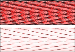
Figure 1 illustrates the role of the endwalls in driving the meridional flow. The plots in the figure are oriented such that the rotating inner cylinder is the left boundary and gravity points downwards. The vortex lines are plotted with levels  $\varGamma \in [0,r_i{\textit {Re}}]$; they appear to be invariant with ${\textit {Re}}$. Instead of isotherms, we have plotted contours of the axial temperature gradient $\partial _z T$, which is a constant $\partial _z T=1/\gamma$ for ${\textit {Re}}=0$, and it clearly highlights the deviations from the initially imposed linear temperature stratification for ${\textit {Re}}\ne 0$. These deviations appear near the corners where the rotating inner cylinder meets the endwalls. For very small ${\textit {Re}}\sim 1$, $\partial _zT$ remains essentially constant and the meridional flow is solely driven by vortex line bending. When the meridional flow is sufficiently strong it is able to modify the temperature stratification, resulting in its baroclinic interaction with the meridional flow. The $(r,z)$-dependence of $\partial _zT$ becomes evident for ${\textit {Re}}\gtrsim 100$, as the meridional flow is focused at the corners. Whereas the azimuthal flow scales as $v\sim {\textit {Re}}$, the meridional flow scales as $(u,w)\sim {\textit {Re}}^{3/2}$, and for ${\textit {Re}}\gtrsim 10$ the meridional flow clearly forms endwall boundary layers whose thickness scales with ${\textit {Re}}^{-1/2}$, as illustrated by the streamlines. These layers are of Bödewadt type, as in isothermal Taylor–Couette flows with stationary endwalls (Avila et al. Reference Avila, Grimes, Lopez and Marques2008).

Figure 1. Contours of  $\varGamma$, $\partial _z T$ and $\psi$ of the steady axisymmetric basic state $S_{0}$ at ${\textit {Re}}$ as indicated. The contour levels (red positive and yellow negative) are $\varGamma \in [0,r_i{\textit {Re}}]$, $\partial _z T \in [0,0.33+4 \times 10^{-4}{\textit {Re}}\,a]$ and $\psi \in [-a,a]$, where $a=0.005+1.3\times 10^{-5}{\textit {Re}}^{3/2}$. Contours are in a meridional plane, $(r,z)\in [r_i,r_o]\times [-\gamma /2,\gamma /2]$.
Often, the basic state is taken to be a unidirectional azimuthal  $z$-independent flow whose $r$ dependence corresponds to the scaled azimuthal velocity of the circular Couette flow between two infinitely long cylinders, together with a linear (in $z$) temperature (density) profile. When the inner cylinder rotates at non-dimensional rate ${\textit {Re}}$ and the outer cylinder is stationary, the circular Couette flow profile is (Taylor Reference Taylor1923)
 \begin{equation} \frac{v(r)}{{\textit{Re}}}= \frac{\eta}{1-\eta^2}\left(\frac{r_o}{r}-\frac{r}{r_o}\right). \end{equation}
Figure 2 compares the radial profiles of the scaled azimuthal velocity  $v/{\textit {Re}}$ at mid-height $z=0$ of the steady axisymmetric state $S_0$ for $\gamma =3$ and ${\textit {Fr}}=0.53$ (for ${\textit {Re}}<500$, this scaled profile at $z=0$ is independent of ${\textit {Re}}$), and of the scaled circular Couette flow (which is independent of ${\textit {Re}}$), both with radius ratio $\eta =0.417$. For the given geometry ( $\eta$ and $\gamma$), the two $v(r)$ profiles are very different. For example, the azimuthal velocities at mid-gap differ by approximately 30 %. This is a well-known consequence of endwall effects (Coles & van Atta Reference Coles and van Atta1966). For much larger aspect ratios, $\gamma \sim \mathcal {O}(10 - 100)$, it is generally expected that the two radial profiles of $v$ are in better agreement, allowing the use of the unidirectional stratified circular Couette flow in linear stability analysis (Boubnov et al. Reference Boubnov, Gledzer and Hopfinger1995, Reference Boubnov, Gledzer, Hopfinger and Orlandi1996; Caton et al. Reference Caton, Janiaud and Hopfinger2000; Molemaker, McWilliams & Yavneh Reference Molemaker, McWilliams and Yavneh2001; Yavneh et al. Reference Yavneh, McWilliams and Molemaker2001; Shalybkov & Rüdiger Reference Shalybkov and Rüdiger2005; Park & Billant Reference Park and Billant2013; Leclercq et al. Reference Leclercq, Nguyen and Kerswell2016a; Robins et al. Reference Robins, Kersalé and Jones2020). However, for short aspect ratios like that studied here, endwall effects drive meridional flows and, as with unstratified Taylor–Couette flows in short aspect ratios, the resulting instabilities can differ significantly (Benjamin & Mullin Reference Benjamin and Mullin1981; Cliffe, Kobine & Mullin Reference Cliffe, Kobine and Mullin1992; Lopez & Marques Reference Lopez and Marques2003; Abshagen et al. Reference Abshagen, Lopez, Marques and Pfister2005a,Reference Abshagen, Lopez, Marques and Pfisterb; Lopez & Marques Reference Lopez and Marques2005; Marques & Lopez Reference Marques and Lopez2006; Abshagen et al. Reference Abshagen, Lopez, Marques and Pfister2008; Lopez Reference Lopez2016).

Figure 2. Radial profiles of the scaled azimuthal velocity  $v/{\textit {Re}}$ at mid-height $z=0$ of the steady axisymmetric state $S_0$ for ${\textit {Re}}\le 500$, $\gamma =3$ and ${\textit {Fr}}=0.53$, and of the scaled azimuthal velocity of the unidirectional circular Couette flow, both for radius ratio $\eta =0.417$.
From figure 1, it is apparent that the steady axisymmetric basic state  $S_0$ is essentially $\mathcal {K}$ symmetric, even though the terms in the governing equations with $\epsilon$ as a factor break the symmetry. As noted earlier, with the choice of fixed parameters under consideration, $\epsilon \propto {\textit {Re}}^2$ with a very small constant of proportionality. As a quantitative measure of the $\mathcal {K}$ symmetry breaking in the flow, we introduce the symmetry measure
 \begin{equation} S_{\mathcal{K}}={\|\boldsymbol{u}-\mathcal{K}\boldsymbol{u}\|_2}/{\|\boldsymbol{u}\|_2}, \end{equation}
where
 \begin{equation} \|({\cdot})\|_2=\sqrt{\int_{-\gamma/2}^{\gamma/2} \int_0^{2\pi} \int_{r_i}^{r_o} ({\cdot})^2 r\,\text{d}r\,\text{d}\theta \,\text{d}z}. \end{equation}
Figure 3 shows that for small  ${\textit {Re}}$, $S_{\mathcal {K}}\sim {\textit {Re}}^4$. For ${\textit {Re}}\lesssim 10$, $S_{\mathcal {K}}$ is essentially machine noise, and for ${\textit {Re}}\gtrsim 100$, $S_{\mathcal {K}}$ grows faster than ${\textit {Re}}^4$, but remains too small for any asymmetry to be evident in figure 1.

Figure 3. Variation of  $S_{\mathcal {K}}$ with ${\textit {Re}}$ for the axisymmetric steady state $S_0$ (blue symbols). For the axisymmetric limit cycle state $L_0$ (green symbols), the time-averaged $S_{\mathcal {K}}$ is shown.
4. Instability of the basic state in the axisymmetric subspace
When the meridional flow is sufficiently large ( $u,w\gtrsim 0.025v$), $S_0$ loses stability via a Hopf bifurcation at ${\textit {Re}}\approx 575$, and a limit cycle state $L_0$ is spawned when the dynamics is restricted to the axisymmetric subspace. Figure 4(a) shows how the kinetic energy in $S_0$ and $L_0$ varies with ${\textit {Re}}$ (for $L_0$ the time-averaged kinetic energy is shown). For $S_0$, $E_0/ {\textit {Re}}^2 \approx 0.52$ whereas for $L_0$ the time-averaged scaled kinetic energy drops with increasing ${\textit {Re}}$. The amplitude of the oscillations in $L_0$ is quantified by the standard deviation in the time series of the kinetic energy, scaled by ${\textit {Re}}^2$; this is shown in figure 4(b). There is near linear growth in the amplitude with increasing ${\textit {Re}}$, starting from zero amplitude at ${\textit {Re}}\approx 590$; this is typical of a supercritical Hopf bifurcation. The frequency of the oscillations, scaled by ${\textit {Re}}$, only varies slightly with ${\textit {Re}}$; this is also typical of a supercritical Hopf bifurcation. This frequency, $\omega _0\approx 0.36{\textit {Re}}$, indicates that the flow oscillates at a frequency that is approximately one third the frequency at which the inner cylinder rotates.

Figure 4. (a) Kinetic energy of solutions computed in the axisymmetric  $m=0$ subspace $E_0$, scaled by ${\textit {Re}}^2$, vs ${\textit {Re}}$. The basic state $S_0$ is steady, and $L_0$ is time periodic (for $L_0$ the time average is plotted). (b) The standard deviation in $E_0$, scaled by ${\textit {Re}}^2$, for $L_0$ and (c) the corresponding frequency $\omega _0$ scaled by ${\textit {Re}}$, vs ${\textit {Re}}$.
Figure 5 shows vortex lines, axial temperature gradient contours and streamlines of  $L_0$ averaged over one period $\tau _0=2\pi /\omega _0$ at various ${\textit {Re}}$, from near onset at ${\textit {Re}}=600$ to ${\textit {Re}}=900$. Near onset, the time-average $\bar {L}_0$ is very similar to the basic state $S_0$ (compare with $S_0$ at ${\textit {Re}}=500$ shown in figure 1); the main difference being that there are cellular structures near the inner cylinder that are most intense near the top and bottom endwall corners and diminishing towards the mid-height region. The time-averaged meridional flow and the deviations away from constant in the time-averaged axial temperature gradients are concentrated in the endwall boundary layers, and in particular near the corners where the endwalls meet the inner cylinder. With increasing ${\textit {Re}}$, the mean meridional flow intensifies, and by ${\textit {Re}}=900$ there is evidence of cellular structure in the interior between the endwalls. The deviations in $\partial _z\bar {T}$ are localized near the inner cylinder, whereas the mean meridional flow extends across the gap between the inner and outer cylinders. This more intense mean meridional flow results in axial oscillations in the mean axial angular momentum $\bar {\varGamma }=r\bar {v}$. For all ${\textit {Re}}$, the mean flow $\bar {L}_0$ is essentially $\mathcal {K}$ invariant, although very small deviations from $\mathcal {K}$ symmetry are evident, particularly in the streamlines at ${\textit {Re}}=800$ and 900 near the mid-height region.

Figure 5. Contours of  $\varGamma$, $\partial _z T$ and $\psi$ of the time-averaged $L_0$ at ${\textit {Re}}$ as indicated. The contour levels (red positive and yellow negative) are $\varGamma \in [0,r_i{\textit {Re}}]$, $\partial _z T\in [0,a]$, where $({\textit {Re}},a)=(600, 0.700)$, (700, 0.627), (800, 0.739), (900, 1.032) and $\psi \in [-b,b]$, where $({\textit {Re}},b)=(600,0.309)$, (700, 0.510), (800, 0.604), (900, 0.627).
Figure 6(a,b) shows space–time plots of the angular momentum  $\varGamma =rv$ and the axial temperature gradient $\partial _z T$ over four periods of $L_0$ at ${\textit {Re}}=600$; the oscillation period is $\tau _0=2\pi /\omega _0\approx 15.93{\textit {Re}}$. Figure 6(c,d) shows snapshots of $\varGamma$ and $\partial _z T$ at eight equispaced times in one period, indicated by the vertical dashed blue lines in the space–time plots. The instantaneous $L_0$ has a well-defined interior cellular structure (see snapshots at $t_0$), but this cellular structure becomes weaker and almost disappears after a quarter period (see snapshots at $t_0+\tau _0/4$), and reappears again after another quarter period (see snapshots at $t_0+\tau _0/2$), but with the cellular structure being the $\mathcal {K}$-symmetric conjugate of the cellular structure at $t_0$. This cycle repeats with period $\tau _0$. This is the reason why the number of cellular structures in the time-average $\bar {L}_0$ (figure 5) is twice the number of cells in $L_{0}$ (figure 6d): the cells at $t_0$ superimposed with the $z$-reflected cells at $t_0+\tau _0/2$ results in doubling the number of cells in the time average. The space–time plots show that the cells are formed at the endwalls and move towards the interior, meeting at the mid-height level. Figure 6 clearly shows that the $\mathcal {K}$ symmetry at any given time is broken. However, there is an almost perfect half-period-flip symmetry: the snapshots after half a period $t+\tau _0/2$ coincide with the $\mathcal {K}$-conjugate snapshots at $t$ (for any $t$), as discussed earlier. A Hopf bifurcation caused by a pair of complex conjugate antisymmetric eigenvectors typically/generically leads to a limit cycle which has this half-period-flip symmetry. Strictly speaking, since the centrifugal term breaks the $\mathcal {K}$ symmetry, there are slight differences that cannot be appreciated in the figure because the breaking of the $\mathcal {K}$ symmetry at this low Reynolds number ( ${\textit {Re}}=600$) is extremely small ( $S_{\mathcal {K}} \sim 10^{-7}$, as shown in figure 3).

Figure 6. The limit cycle  $L_0$ at ${\textit {Re}}=600$: space–time $(t,z)$ contour plots of (a) $\varGamma$ and (b) $\partial _z T$ at $\theta =0$ and $r=r_i+0.1$; four periods are shown, where $\tau _0=2\pi /\omega _0\approx 15.92/{\textit {Re}}$ is the period of $L_0$. The corresponding meridional snapshots at indicated times corresponding to the eight equispaced vertical dashed blue lines in (a,b) are shown in (c,d). Supplementary movie 1 animates the $\varGamma$ and $\partial _z T$ contours in the meridional plane over one period.
Figure 7 shows the corresponding plots from figure 6 for  $L_0$ at ${\textit {Re}}=800$. It is evident that instead of having an approximate half-period-flip symmetry (i.e. setwise $\mathcal {K}$ invariance), the flow at this ${\textit {Re}}$ is pointwise-in-time $\mathcal {K}$ invariant. This type of switching between stable limit cycles bifurcating from a basic state with $\mathcal {K}$ symmetry to periodic states that either have pointwise-in-time $\mathcal {K}$ symmetry ( $L_0$ at ${\textit {Re}}=800$) or setwise-in-time (half-period-flip) symmetry ( $L_0$ at ${\textit {Re}}=600$) is commonly observed in $\mathcal {K}$ (or related $Z_2$) symmetric systems (e.g. Marques & Lopez Reference Marques and Lopez2015; Yalim, Welfert & Lopez Reference Yalim, Welfert and Lopez2019; Grayer et al. Reference Grayer, Yalim, Welfert and Lopez2020). Strictly speaking, in the present problem the $\mathcal {K}$ symmetry is broken due to the centrifugal buoyancy, as has already been discussed. This symmetry breaking is very weak, but at ${\textit {Re}}=800$, a close inspection of some of the snapshots in figure 7(d) near the mid-height shows clear evidence of the symmetry breaking. The cellular structures at ${\textit {Re}}=800$ are more pronounced than at ${\textit {Re}}=600$ as $L_0$ is further away from onset.

Figure 7. The limit cycle  $L_0$ at ${\textit {Re}}=800$: space–time $(t,z)$ contour plots of (a) $\varGamma$ and (b) $\partial _z T$ at $\theta =0$ and $r=r_i+0.1$; four periods are shown, where $\tau _0=2\pi /\omega _0\approx 17.67/{\textit {Re}}$ is the period of $L_0$. The corresponding meridional snapshots at indicated times corresponding to the eight equispaced vertical dashed blue lines in (a,b) are shown in (c,d). Supplementary movie 1 animates the $\varGamma$ and $\partial _z T$ contours in the meridional plane over one period.
While the snapshots in figures 6 and 7 are instructive, the animations of the fields (see supplementary movie 1 available at https://doi.org/10.1017/jfm.2021.893) illustrate the dynamics better. Twice every period, a new cell is formed at each of the corners where the endwalls meet the inner cylinder. The new cells propagate axially into the interior, pushing the existing cells further toward the mid-plane  $z=0$, resulting in the annihilation of the angular momentum jets and cells. The jets reappear in other places, with either the same or a different number of cells, depending on the symmetry of $L_0$. Jets of angular momentum, which are characteristic of the centrifugal instability due to the inner cylinder rotation, are clearly observed. During a period, these jets intensify, become weaker, disappear and then reappear with their radial direction inverted, i.e. the outgoing jets become ingoing jets and vice versa (see, for example, the snapshots in figure 7c at times $t_0+\tau _0/4$ and $t_0+3\tau _0/4$). There is a pair of counter-rotating Taylor vortices between two adjacent outgoing jets, forming a Taylor cell, as illustrated in figure 8(d,e), showing the meridional velocity field of $L_0$ at ${\textit {Re}}=800$, at the two times $t_0+\tau _0/4$ and $t_0+3\tau _0/4$, when the jets are most intense. Instantaneous streamlines, axial temperature gradient and angular momentum contours are also shown in the figure, and movie 1 animates these over one period.

Figure 8. The limit cycle  $L_0$ at ${\textit {Re}}=800$, showing $\varGamma$, $\partial _z T$, $\psi$ and velocity vectors projected onto a meridional plane at two times, (a,b,c,d) and (h,g,f,e), half a period apart, during which the outgoing radial jets are strongest.
The Taylor cell boundaries (i.e. the outgoing jets) are indicated by red lines in figure 8. These boundaries are flat, except near the endwalls where the intense Ekman layers with strong velocities near the corners at the inner cylinder distort the adjacent cell boundaries. Each Taylor cell consists of a pair of counter-rotating Taylor vortices. The axial wavelength  $\lambda$ (i.e. the axial height of the Taylor cell relative to the annular gap) is invariant along the cylinder (except very near the Ekman layers), and it remains unchanged in time, even following the switching between ingoing and outgoing jets. This wavelength is much smaller than the wavelength of Taylor cells in unstratified Taylor-vortex flow, which typically have $\lambda _{TVF}\sim 2$ (the Taylor vortices tend to have a square cross-section). Since the flow is divergence free, the strong radial flows in the cells must have axial components to complete the circuits, but the stratification tends to inhibit axial flow, and so the axial flow is constrained to the boundary layers on the inner and outer cylinders. The axial flow on the inner cylinder, together with the radial flow there, leads to the isotherms being advected to the borders of the cells such that where the axial flow converges at these borders, the isotherms are concentrated axially, resulting in a step-like layering. For $L_0$ at ${\textit {Re}}=800$, $\lambda \approx 0.415$; the stratification inhibits the axial motions and reduces the axial span of the cells to approximately $1/5$ of $\lambda _{TVF}$.
The outgoing jets are associated with intense axial temperature gradients, as shown in figure 8. Figure 7(b) shows a space–time plot of  $\partial _z T$; the white ovals are regions of constant temperature ( $\partial _z T=0$), separated by narrow axial regions of large axial temperature gradients, corresponding to the narrow radial ‘jets’ of $\partial _z T$ in figure 8. The temperature has a ‘staircase’ structure (step-like layering) near the inner cylinder (between the inner cylinder and the mid-gap), with regions of constant temperature (the Taylor cells) separated by narrow regions of large axial temperature gradient coinciding with the centres of the outgoing jets. The stratification changes periodically with time and the layering appears and disappears periodically in different axial locations. These step-like layers are confined near the cylinder; this is the region where the centrifugal instability mechanism is most active. The layering does not have time to propagate radially out to the outer cylinder due to the temporal oscillations of the jets. During the short time intervals when the angular momentum jets disappear, the temperature stratification becomes mostly uniform in the axial direction, as shown in figure 7.
The switching between ingoing and outgoing jets results in a different number of Taylor cells, changing between 5 and 6 cells for  $L_0$ at ${\textit {Re}}=800$. The cell boundaries are indicated by red lines in figure 8. The axial size of the cells, $\lambda$, does not vary during the switching: the Ekman vortices at the endwalls change size in order to accommodate a different number of cells. The size of the Ekman vortices is indicated in green in figure 8. When the Ekman vortex is large, it develops an outgoing jet of angular momentum in its interior that propagates axially from the endwall, resulting in the switching between different number of cells.
When the Ekman layer is small (figure 8e) the radial velocity at the endwalls is inwards. This is what has been called in many studies of Taylor–Couette flow a normal mode (Benjamin & Mullin Reference Benjamin and Mullin1981; Cliffe et al. Reference Cliffe, Kobine and Mullin1992; Watanabe, Furukawa & Nakamura Reference Watanabe, Furukawa and Nakamura2002; Lopez & Marques Reference Lopez and Marques2005; Marques & Lopez Reference Marques and Lopez2006). When the Ekman layer is large (figure 8d) the radial velocity at the endwalls is outwards, as in a so-called anomalous mode. This switching is typical of many Taylor–Couette flows of finite axial extent. For  $L_0$ at ${\textit {Re}}=800$, the switching between normal and anomalous mode types occurs twice every oscillation period. It is worth mentioning that even during the anomalous mode phase, there is still a small corner vortex near the inner cylinder so that the radial velocity is locally inwards (figure 8d).
We have described the flow of  $L_0$ at ${\textit {Re}}=800$ in more detail than that of $L_0$ at ${\textit {Re}}=600$ because the jets, cellular structures and staircase temperature profiles are much more evident. In figure 9 for $L_0$ at ${\textit {Re}}=600$ we observe similar cellular structures, and jets of angular momentum as at ${\textit {Re}}=800$. However, due to the different symmetry of the flow, the behaviour of the Ekman cells is different. In the ${\textit {Re}}=800$ case, with $\mathcal {K}$ symmetry, both Ekman layers have the same size and when their size changes, the number of cells also changes. In the ${\textit {Re}}=600$ case, when one of the Ekman layers grows, the other shrinks, and as a result the number of cells does not change. The cells become weaker, disappear, and then reappear with the radial direction of the jets inverted, as in the ${\textit {Re}}=800$ case. For ${\textit {Re}}=600$, there is just an axial oscillation of the cells, combined with their formation/vanishing. The wavelength is constant all the time, $\lambda \approx 0.423$. Compared with the ${\textit {Re}}=800$ case ( $\lambda \approx 0.415$) we see that the cell size does not change very much with ${\textit {Re}}$, there is a small decrease in $\lambda$ with increasing ${\textit {Re}}$. Also, for the half-period-flip symmetric $L_0$ at ${\textit {Re}}=600$, one Ekman layer is in the normal mode phase while the other is in the anomalous mode phase. There is still a pair of persistent corner vortices maintaining the radial flows into the corner on both endwalls.

Figure 9. The limit cycle  $L_0$ at ${\textit {Re}}=600$ showing $\varGamma$, $\partial _z T$, $\psi$ and velocity vectors projected onto a meridional plane at two times, (a,b,c,d) and (h,g,f,e), half a period apart, during which the outgoing radial jets are strongest.
5. Three-dimensional instability of the basic state
In the previous section, the primary instability of the basic state  $S_0$ was explored by restricting the flow to the axisymmetric subspace. Without making such a restriction, $S_0$ loses stability at a lower ${\textit {Re}}\approx 320$ via a Hopf bifurcation breaking the $SO(2)$ symmetry, leading to a rotating wave with azimuthal wavenumber $m=1$, denoted $R_1$. Figure 10(a) shows how the modal kinetic energy in $m=1$, scaled by ${\textit {Re}}^2$, increases linearly from zero at onset and saturates nonlinearly by ${\textit {Re}}\approx 700$. For ${\textit {Re}}\gtrsim 1000$, the rotating wave has a low-amplitude long-period irregular modulation (this modulated rotating wave, $MR_1$, is described below). For $MR_1$, the reported modal energies are time averaged. Figure 10(b) shows the scaled modal kinetic energy in the axisymmetric component of the flow, $E_0/{\textit {Re}}^2$. It is two orders of magnitude larger than $E_1/{\textit {Re}}^2$. For the rotating waves, $E_1/{\textit {Re}}^2$ is a measure of their amplitude, just as the scaled standard deviation in $E_0$ was a measure of the oscillation amplitude of $L_0$ (figure 4b); these two amplitudes are of comparable magnitude. Figure 10(c) shows the precession frequency of the rotating wave scaled by ${\textit {Re}}$, $\omega _p/{\textit {Re}}$. It decreases slowly with increasing ${\textit {Re}}$, but remains close to one third of the rotation frequency of the inner cylinder. This is similar to the behaviour of the oscillation frequency $\omega _0$ of $L_0$ (see figure 4c), but $\omega _p$ is a little smaller than $\omega _0$ overall.

Figure 10. Variation with  ${\textit {Re}}$ of the scaled modal kinetic energies in azimuthal wavenumber (a) $m=1$, $E_1/{\textit {Re}}^2$ and (b) $m=0$, $E_0/{\textit {Re}}^2$, (c) the scaled precession frequency $\omega _p/{\textit {Re}}$ of the rotating wave $R_1$ (red symbols) and modulated rotating waves $MR_1$ (yellow symbols), all for ${\textit {Fr}}\approx 0.53$. (d) The symmetry measures $S_{\mathcal {K}}$ and $S_{\mathcal {C}}$ of these states, and (e) axial wavelength, $\lambda$, measured at $r=r_i+0.1$ near mid-height $z=0$.
For the small  ${\textit {Re}}$ at which the Hopf bifurcation spawning $R_1$ occurs when ${\textit {Fr}}\approx 0.53$, the imperfection in the $\mathcal {K}$ symmetry about the axial mid-plane is essentially negligible; $S_{\mathcal {K}}=2.9\times 10^{-11}$ for the base state $S_0$ at ${\textit {Re}}=340$. Along with the $SO(2)$ symmetry, the $\mathcal {K}$ symmetry is also broken at the bifurcation leading to a rotating wave $R_1$ that has centrosymmetry (albeit imperfect due to $\epsilon \approx 2.4\times 10^{-4}$ being small but not zero). The action of centrosymmetry, $\mathcal {C}=\mathcal {R}_\pi \mathcal {K}=\mathcal {K}\mathcal {R}_\pi$, is
 \begin{equation} \mathcal{C}:[u,v,w,T](r,\theta,z,t)\mapsto[u,v,-w,-T](r,\theta-\pi,-z,t), \end{equation}
and for a rotating wave with azimuthal wavenumber  $m=1$ and precession frequency $\omega _1$,
 \begin{equation} [u,v,w,T](r,\theta-\phi,z,t)=[u,v,w,T](r,\theta,z,t+\phi/\omega_1). \end{equation}
For a rotating wave, the centrosymmetry  $\mathcal {C}$ is the same as the half-period-flip symmetry because a rotation of $\pi$ is the same as advancing half a period in time. As a quantitative measure of the $\mathcal {C}$ centrosymmetry, we introduce the symmetry measure
 \begin{equation} S_{\mathcal{C}}={\|\boldsymbol{u}-\mathcal{C}\boldsymbol{u}\|_2}/{\|\boldsymbol{u}\|_2}. \end{equation}
Figure 10(d) shows the symmetry measures  $S_{\mathcal {K}}$ and $S_{\mathcal {C}}$ of $R_1$ and $MR_1$. For the rotating waves at ${\textit {Re}}\leq 1000$, one or the other symmetry measure is very small (of order $10^{-6}$) while the other grows from near zero to 0.2 with increasing ${\textit {Re}}$. The rotating wave $R_1$ comes in two flavours, one $\mathcal {C}$ symmetric and the other $\mathcal {K}$ symmetric, and alternates between the two cases as ${\textit {Re}}$ is increased. This is analogous to switching between setwise and pointwise-in-time $\mathcal {K}$ invariance for the axisymmetric limit cycle $L_0$. The $\mathcal {C}$ symmetry is the purely spatial version of the half-period-flip symmetry. It is very likely that the underlying mechanisms for the symmetry-type switching with increasing ${\textit {Re}}$ in $L_0$ and $R_0$ are the same, and tied to the underlying $\mathcal {K}$ symmetry of the basic state $S_0$.
Figure 10(e) shows the variation of the axial wavelength  $\lambda$ of the Taylor cells. It is measured as the distance between the peaks of azimuthal temperature gradient $\partial _zT$ closest to mid-height $z=0$ (i.e. away from the endwalls and the distorting effects of the Ekman vortices), near the inner cylinder (at $r=r_i+0.1$). Figure 8 shows a typical example for $L_0$, illustrating where $\lambda$ has been measured. The wavelength $\lambda$ steadily decreases linearly with ${\textit {Re}}$ for $R_1$ (except for the first point very near the bifurcation ${\textit {Re}}\approx 340$, where the Taylor cells are weak and $\lambda$ is difficult to measure). In contrast, for ${\textit {Re}}>1000$ the wavelength of the modulated rotating waves $MR_1$ remains almost independent of ${\textit {Re}}$ with $\lambda \sim 0.4$.
Figure 11(a,b) shows space–time plots of  $\varGamma$ and $\partial _z T$ along an axial line at $(r,\theta,z)=(r_i+0.1,0,z)$ over four precession periods of $R_1$ at ${\textit {Re}}=500$; the precession period is $\tau _p=2\pi /\omega _p\approx 17.85{\textit {Re}}$. These space–time plots can also be viewed as $(\theta,z)$ plots because $R_1$ is a rotating wave (the time $t\in [t_0,t_0+4\tau _p]$ being replaced with $\theta \in [0,8\pi ]$). The figure shows the same features as in the space–time plots for $L_0$: there are regions of constant temperature (white regions in figure 11a) bounded in $z$ by regions of large axial temperature gradient – the staircase temperature profiles described earlier for $L_0$. Figure 11(c,d) shows snapshots, in the meridional plane $\theta =0$, of $\varGamma$ and $\partial _z T$ at eight equispaced times over one period (or equivalently, in eight equispaced meridional planes with $\theta \in [0,2\pi ]$, all at the same instant in time), indicated by the vertical dashed blue lines in the space–time plots. The rotating wave $R_1$ at ${\textit {Re}}=500$ is essentially $\mathcal {C}$ symmetric ( $S_{\mathcal {C}}=4.14 \times 10^{-6}\approx 0$ and $S_{\mathcal {K}}=0.105\ne 0$). The outgoing jets of angular momentum, coinciding with the regions of large axial temperature variation, are clearly evident. Over one period in a particular meridional plane, these jets become weaker, disappear and then reappear with the direction of their radial velocity reversed. However, for $R_1$ these structures remain invariant in time and simply rotate continuously in azimuth. In contrast, for $L_0$ the formation and destruction of the jets and sharp axial temperature gradients occurs globally in azimuth and periodically in time. The $R_1$ jets are essentially $\theta$-invariant for $\theta _0\lesssim \theta \lesssim \theta _0+\pi$ and for $\theta _0+\pi \lesssim \theta \lesssim \theta _0+2\pi$, but displaced axially by $\lambda /2$ in the two azimuthal halves, with narrow bands of ‘defects’ connecting the jets in the two halves.

Figure 11. The rotating wave  $R_1$ at ${\textit {Re}}=500$: space–time $(t,z)$ contour plots of (a) $\varGamma$ and (b) $\partial _z T$ at $\theta =0$ and $r=r_i+0.1$; four precession periods are shown, where $\tau _p=2\pi /\omega _p\approx 17.85/{\textit {Re}}$ is the precession period of $R_1$. The corresponding meridional snapshots at indicated times corresponding to the eight equispaced vertical dashed blue lines in (a,b) are shown in (c,d).
Figure 12(a,b) shows space–time plots of  $\varGamma$ and $\partial _z T$ over four precession periods of $R_1$ at ${\textit {Re}}=800$; the precession period is $\tau _p=2\pi /\omega _p\approx 18.65{\textit {Re}}$. Figure 12(c,d) shows snapshots of $\varGamma$ and $\partial _z T$ at eight equispaced times in one period, indicated by the vertical dashed blue lines in the space–time plots. The value of $R_1$ at ${\textit {Re}}=800$ is essentially $\mathcal {K}$ symmetric ( $S_{\mathcal {K}}=2.14\times 10^{-5}\approx 0$ and $S_{\mathcal {C}}=0.163 \ne 0$). The same considerations as for $R_1$ at ${\textit {Re}}=500$ apply here, the only difference being the different symmetry of the solution. Figure 13 shows snapshots of $\varGamma$ and $\partial _zT$ isosurface, one quarter period apart, illustrating the three-dimensional structure of $R_1$ at ${\textit {Re}}=500$ and 800. Supplementary movie 2 shows animations of these over one precession period; these animations provide clearer insights into the flow structures.

Figure 12. The rotating wave  $R_1$ at ${\textit {Re}}=800$: space–time $(t,z)$ contour plots of (a) $\varGamma$ and (b) $\partial _z T$ at $\theta =0$ and $r=r_i+0.1$; four precession periods are shown, where $\tau _p=2\pi /\omega _p\approx 18.65/{\textit {Re}}$ is the period of $R_1$. The corresponding meridional snapshots at indicated times corresponding to the eight equispaced vertical dashed blue lines in (a,b) are shown in (c,d).

Figure 13. Isosurfaces of  $\varGamma$ and $\partial _z T$ of $R_1$ at ${\textit {Re}}=500$ and 800, at two different times a quarter precession period apart. The isolevels are $\varGamma =0.4r_i{\textit {Re}}$ and $\partial _z T=0.493$ (which is $30\,\%$ of the maximum axial temperature gradient) for $\textit{Re} =500$ and $\partial _z T=0.625$ (which is $22\,\%$ of the maximum axial temperature gradient) for ${\textit {Re}}=800$. Supplementary movie 2 includes an animation of these over one precession period.
Figure 14 shows vortex lines, axial temperature gradient contours and streamlines of  $R_1$ averaged over one period $\tau _0=2\pi /\omega _0$ (or equivalently, averaged with respect to $\theta$) at various ${\textit {Re}}$, from near onset at ${\textit {Re}}=340$ to ${\textit {Re}}=1000$. The plots are very similar to those in figure 5 for the time-averaged $L_0$. The only significant difference is that the cellular structures are more intense and the jets of angular momentum (and the associated staircase structures in the temperature) penetrate radially further in from the inner cylinder for $R_1$ than they do for $L_0$.

Figure 14. Contours of  $\varGamma$, $\partial _z T$ and $\psi$ of the time-averaged $R_1$ at ${\textit {Re}}$ as indicated. The contour levels (red positive and yellow negative) are $\varGamma \in [0,r_i{\textit {Re}}]$, $\partial _z T\in [0,0.2+7.5\times 10^{-4}{\textit {Re}}]$ and $\psi \in [-b,b]$, where $b=-0.09+2.3\times 10^{-5}{\textit {Re}}^{3/2}$.
For  ${\textit {Re}}>1000$, centrifugal buoyancy effects are stronger, leading to greater asymmetry between the two rotating waves associated with the upper and lower corners. They now have slightly different precession frequencies, resulting in a quasiperiodic modulated rotating wave, $MR_1$. The modulation is a very low frequency beating on the underlying rotating wave. Figure 15 shows time series of the modal kinetic energy $E_1$ scaled by ${\textit {Re}}^2$ and the corresponding power spectral densities for $R_1$ at ${\textit {Re}}=1000$ and $MR_1$ at a selection of larger ${\textit {Re}}$. They clearly show the appearance of a very low frequency $\omega _2$. More importantly, the primary peak is associated with the precession frequency of the underlying rotating wave, $\omega _p\approx 0.32$ with a very small decrease with increasing ${\textit {Re}}$; the power in this primary peak is almost two orders of magnitude larger than the power in the very low frequency modulation peak. As such, the modulations are weak and manifest over hundreds of inner cylinder rotations.

Figure 15. Time series (a) of the modal kinetic energy  $E_1/{\textit {Re}}^2$, and (b) power spectral density (PSD) of the azimuthal component of velocity at a point $(r,\theta,z)=(r_i+0.1,0,0.25\gamma )$, for ${\textit {Fr}}\approx 0.53$ and ${\textit {Re}}$ as indicated.
Figure 16 shows space–time plots of  $\varGamma$ and $\partial _z T$ over four precession periods for $R_1$ at ${\textit {Re}}=1000$ and $MR_1$ at a selection of larger ${\textit {Re}}$. The main feature of these spatio-temporal structures is the presence of the staircase structures, with very narrow regions of fast variation of temperature, separated by regions of almost constant temperature, as shown in the second column of figure 16. These structures, and the associated outgoing jets of angular momentum, are distorted with increasing ${\textit {Re}}$, and the $\mathcal {C}$ and $\mathcal {K}$ symmetries are completely broken. The propagation towards the interior of the perturbations generated at each endwall is clearly evident. Some of the plots show that the waves propagating from the top endwall fill most of the interior (as in figure 16b for ${\textit {Re}}=1250$), and others show the opposite (as in figure 16c for ${\textit {Re}}=1500$). In fact, the dominance of one or other of the endwalls changes very slowly in time, corresponding to the very low frequency $\omega _2$ of $MR_1$. This is due to the detuning between the oscillation frequencies of the Ekman vortices at the endwalls. This type of behaviour was also observed in Lopez & Marques (Reference Lopez and Marques2020), with smaller radius ratio and larger stratification. The spatio-temporal plots in figure 16 are also very similar to those reported from experiments using salt stratification in a Taylor–Couette apparatus with very similar radius and aspect ratios (Partridge et al. Reference Partridge, Leclercq, Caulfield and Dalziel2016), as well as in experiments using temperature stratification with oil and quite larger radius ratio $\eta \approx 0.52$ and aspect ratio $\gamma \approx 10$ (Meletti et al. Reference Meletti, Abide, Viazzo, Krebs and Harlander2021). This suggests that the Prandtl number (which varies from approximately 700 for salt stratification, approximately 57 for the oil, to approximately 6 for temperature stratification in water) does not play a critical role in the layering pattern selection process.

Figure 16. Space–time contour plots  $(t,z)$ of $\varGamma$ (left) and $\partial _z T$ (right) at $\theta =0$ and $r=r_i+0.1$ over four precession periods for $R_1$ and $MR_1$ at ${\textit {Re}}$ as indicated. Three (eight) contour levels between 0 and the maximum value for $\partial _z T$ ( $\varGamma$).
Figure 17 illustrates the changes in flow structure associated with the very low frequency  $\omega _2\approx \omega _p/20$ for $MR_1$ at ${\textit {Re}}=1250$. It includes time series of the axial velocity $w$ at three points in a meridional plane, $\theta =0$, very close to the inner cylinder, $r=r_i+0.01$, at three heights, $z=0$ and $z=\pm 0.5\gamma$, as well as time series of the symmetry measures $S_{\mathcal {C}}$ and $S_{\mathcal {K}}$. The time series are shown over one viscous time, which is approximately three times $2\pi /\omega _2$. Over most of each $2\pi /\omega _2$ period, the flow has a regular almost periodic behaviour during which it is approximately $\mathcal {K}$-symmetric ( $S_{\mathcal {K}}\approx 0$). As a consequence, the axial velocity $w$ at $z=0$ is approximately zero and $w|_{z=0.5\gamma }\approx -w|_{z=-0.5\gamma }$. This regular, nearly $\mathcal {K}$-symmetric phase is followed by an irregular shorter phase during which the reflection symmetry measure $S_{\mathcal {K}}$ increases to be approximately a fifth of $S_{\mathcal {C}}$; $S_{\mathcal {C}}$ also increases ever so slightly during this phase. The yellow symbols in the time series in figure 17 are strobed with the precession frequency $\omega _p$, and the isosurfaces of $\partial _zT$ at these strobed times are shown in supplementary movie 3. Fifteen equispaced snapshots (five per period $2\pi /\omega _2$) are shown in figure 17(f). The first three snapshots in each row (each row covers one $2\pi /\omega _2$ period) show very little variation, corresponding to the regular phase of $MR_1$, with almost $\omega _p$-periodic behaviour. The last two snapshots correspond to the irregular phase, with rapid changes in the flow. The (strobed) position of the defect at mid-height remains constant during the regular phase, while it experiences a jump during the irregular phase; this jump coincides with $\mathcal {K}$-symmetry breaking. This behaviour is a ‘snapping’ of the defect; it was also observed in very wide-gap stratified Taylor–Couette flow (Lopez & Marques Reference Lopez and Marques2020), in which both curvature and centrifugal buoyancy effects were much stronger than in the present problem. There, the ‘snapping’ was related to the detuning of the frequencies associated with the centrifugal instabilities near the endwalls. This effect was large in that study, and affected the first instability of the flow. In the present problem, centrifugal buoyancy effects begin to manifest well beyond the onset of instability (for ${\textit {Re}}>1000$ compared with onset at ${\textit {Re}}\approx 320$), and result in the transition to modulated rotating waves $MR_1$. Further increases in ${\textit {Re}}$ above ${\textit {Re}}\approx 2000$ results in complex spatio-temporal behaviour, as the time series and power spectral densities in figure 15 indicate.

Figure 17. The modulated rotating wave  $MR_1$ at ${\textit {Re}}=1250$: (a–c) time series of the axial velocity $w$ at $(r,\theta )=(r_i+0.05,0)$ and $z$ as indicated, over one viscous time covering three periods of $\omega _2$; (d,e) time series of the symmetry measures $S_{\mathcal {C}}$ and $S_{\mathcal {K}}$. The yellow symbols are strobed at the precession frequency $\omega _p$, and correspond to the frames in movie 3. (f) Frames selected from movie 3, showing isosurfaces of $\partial _z T$ at times indicated by red symbols in (a) to (e).
6. Discussion and conclusions
We have presented a detailed study of the onset of instability of stratified Taylor–Couette flow in an annulus with medium radius ratio,  $\eta =0.417$, and short aspect ratio, $\gamma =3$, inspired by a series of experiments (Oglethorpe et al. Reference Oglethorpe, Caulfield and Woods2013; Leclercq et al. Reference Leclercq, Partridge, Augier, Caulfield, Dalziel and Linden2016b,Reference Leclercq, Partridge, Caulfield, Dalziel and Lindend; Partridge et al. Reference Partridge, Leclercq, Caulfield and Dalziel2016). This is a very different geometry to that usually studied, where the aspect ratio is large to minimize endwall effects and the radius ratio is large ( $\eta \sim 1$) to minimize curvature effects (e.g. Boubnov et al. Reference Boubnov, Gledzer and Hopfinger1995; Le Bars & Le Gal Reference Le Bars and Le Gal2007; Ibanez et al. Reference Ibanez, Swinney and Rodenborn2016). As in unstratified Taylor–Couette flow in a finite annulus, the instability initiates at the corners where the inner rotating cylinder meets the stationary endwalls. From there, it propagates axially into the interior along the inner cylinder. This process is (up-down) $\mathcal {K}$ symmetric in the absence of stratification. However, with stratification the centrifugal buoyancy breaks the $\mathcal {K}$ symmetry, albeit weakly near onset of instability for the parameter regimes considered in this study.
In similar stratified Taylor–Couette flows with smaller radius ratio,  $\eta \approx 0.07$, and stronger stratification (Flór et al. Reference Flór, Hirschberg, Oostenrijk and van Heijst2018; Lopez & Marques Reference Lopez and Marques2020), the corner vortices emit spiral waves with small inclination towards the interior. The frequencies of these spiral waves emitted from the top and bottom endwalls are slightly different due to the imperfect $\mathcal {K}$ symmetry, although the frequencies lock near the bifurcation point resulting is single frequency periodic flow. In the present problem, with larger $\eta =0.417$, the spiral waves are not present, and the instability takes the form of what may loosely be described as flat Taylor vortices with small axial wavelength that are not axisymmetric; they are broken in half azimuthally and the halves are axially displaced approximately half a wavelength (this is reminiscent of the experimental observations by Boubnov et al. (Reference Boubnov, Gledzer, Hopfinger and Orlandi1996)). So, like the helical waves in the small $\eta$ flows, they have azimuthal wavenumber $m=1$, but they are not smooth helical waves.
In both the small  $\eta$ study (Lopez & Marques Reference Lopez and Marques2020) and the present medium $\eta$ study, the ratio of rotation to buoyancy frequency was ${\textit {Fr}}=0.53$. However, in the much smaller $\eta$ case the helical waves from the instability remain localized to the rotating inner cylinder, and their onset is at ${\textit {Re}}\sim 6\times 10^{3}$. This critical ${\textit {Re}}$ is twenty times larger than for the medium $\eta =0.417$ studied here. As a consequence, the effects of centrifugal buoyancy near onset are much weaker in the present study. In the small $\eta$ experiments (Flór et al. Reference Flór, Hirschberg, Oostenrijk and van Heijst2018) and numerical simulations (Lopez & Marques Reference Lopez and Marques2020), centrifugal buoyancy leads to the lower corner losing stability at a lower ${\textit {Re}}$ than the top corner, and these localized perturbations have slightly different frequencies. However, in the present medium $\eta$ study, it appears that due to viscous effects together with the small value of $\epsilon \sim 10^{-4}$ (quantifying the strength of the centrifugal buoyancy), the two instability wave frequencies lock and the whole flow is a single frequency periodic flow (a rotating wave) over a wide range of ${\textit {Re}}$, from onset at ${\textit {Re}}\approx 340$ up to ${\textit {Re}}=1000$. In laboratory experiments, which often use salt stratification in an annulus with a no-slip bottom and an open top, the up–down $\mathcal {K}$ symmetry is further broken. The details of how the symmetry is broken lead to a very complicated dynamics in a very small neighbourhood of the onset of instability, but further beyond onset the symmetry-broken dynamics becomes less dependent on the details (Pacheco, Lopez & Marques Reference Pacheco, Lopez and Marques2011; Marques et al. Reference Marques, Meseguer, Lopez, Pacheco and Lopez2013).
Perhaps more important than accounting for centrifugal buoyancy effects is to account for the presence of endwalls in the short aspect ratio,  $\gamma =3$, flows. Endwalls are ignored when studying the linear stability so that a basic unidirectional basic state can be considered; we have shown how different the basic state is in the short finite length annulus. When considering the nonlinear dynamics ignoring endwalls, nonlinear flows are assumed to be axially periodic (with the axial period often being assigned to be the wavelength of the most unstable mode or some integer multiple of that wavelength). The axially periodic system has $SO(2)\times O(2)$ symmetry, where $SO(2)$ corresponds to invariance to rotations about the axis and $O(2)=SO(2)\rtimes Z_2$ corresponds to arbitrary axial translations, $SO(2)$, and reflections about any axial level, $Z_2$. In the finite annulus, ignoring centrifugal buoyancy, the system has $SO(2)\times Z_2$ symmetry, with $Z_2$ being the mid-height reflection. With the idealized $O(2)$ symmetry, the primary non-axisymmetric instability in stratified Taylor–Couette flows is to spiral waves of opposite chirality, called ribbons, or if the axial symmetry is broken then mixed-ribbons or cross-spirals result (Leclercq et al. Reference Leclercq, Partridge, Augier, Caulfield, Dalziel and Linden2016b). Without endwalls, these nonlinear states can have a non-zero net axial mass flux. The presence of endwalls (or even if the top surface is open) enforces a zero net axial mass flux. For very large aspect ratios, this can be enforced numerically by allowing a finite axial pressure gradient which recovers the correct global recirculation in the capped annulus (Marques & Lopez Reference Marques and Lopez1997), but for short aspect ratio annuli, it is easier and more correct to directly model the endwalls, as is done in the present study. Furthermore, stratified flow in an axially infinite annulus is conceptually problematic, particularly within the Boussinesq approximation.
One of the more spectacular features of the stratified Taylor–Couette flows studied here is the formation of layers immediately following the onset of instability. These layers – regions of uniform density separated by much thinner regions of large axial density gradient – are observed in many stratified shear flows, but there is no general consensus on how they come about nor on how their length scales are set (see Thorpe (Reference Thorpe2016), for a discussion of various candidate mechanisms). There continues to be great interest in addressing these open questions (Caulfield Reference Caulfield2020, Reference Caulfield2021), as is reflected in a recent research program (Diamond et al. Reference Diamond, Garaud, Hughes and Sutherland2021), where the  $\eta =0.417$, $\gamma =3$ stratified Taylor–Couette flow was held up as an example laboratory experiment in which this layering is observed. There remain open questions, such as whether linear instability sets the layering scales. The results of our simulations of this flow at least establish that the primary instability – resulting from the competition between a Rayleigh unstable angular momentum distribution, stable stratification inhibiting axial variations and viscous damping – does account for the spatio-temporal layered structures. The large density gradients occur precisely where the strong radial jets of angular momentum leaving the inner cylinder boundary layer form. Near onset, the axial spacing between these jets is $\lambda \approx 0.6$, corresponding to five jets in the $\eta =0.417$, $\gamma =3$ annulus, and the number of jets increase with ${\textit {Re}}$. The jets are not axisymmetric, they have azimuthal wavenumber $m=1$ but are not smooth in azimuth. They precess in azimuth at approximately one third the rotation rate of the inner cylinder, with this precession rate a slowly decreasing function of ${\textit {Re}}$.
Supplementary movies
Supplementary movies are available at https://doi.org/10.1017/jfm.2021.893.
Funding
This work was supported by the Spanish Ministry of Education and Science/FEDER grants FIS2017-85794-P and PRX18/00179.
Declaration of interests
The authors report no conflict of interest.


 Open access