


1. Introduction
1.1. Jet screech
It has long been observed that shock-containing supersonic jets resonate at a distinct fundamental tone with accompanying harmonics in a phenomenon known as jet screech. This phenomenon is underpinned by a resonance feedback loop involving waves that propagate both upstream and downstream (Powell Reference Powell1953; Edgington-Mitchell Reference Edgington-Mitchell2019). Four processes are involved in the feedback loop. The loop is initialised by a downstream propagation of energy, usually in the form of a hydrodynamic disturbance. This is followed by a mechanism in which energy associated with the downstream-propagating disturbance is converted to an upstream-propagating disturbance, typically generating the acoustic tone. The upstream propagation perturbs a sensitive point in the base flow, forcing it to produce new downstream-propagating waves and, therefore, closing the feedback loop.
Within the context of a single jet, variation in Mach number leads to two interlinked phenomena: discontinuous changes in frequency referred to as ‘staging’ and different azimuthal modes (Edgington-Mitchell Reference Edgington-Mitchell2019). The frequency staging has multiple acoustic branches labelled A1, A2, B, C and D; A1 and A2 correspond to axisymmetric ( $m = 0$) modes, while B, C and D modes correspond to flapping or helical ( $m = 1$). With the addition of a second jet – a twin-jet configuration – jet screech is strongly amplified, with levels significantly higher than the doubling expected from a linear superposition (Seiner, Manning & Ponton Reference Seiner, Manning and Ponton1988; Raman et al. Reference Raman, Panda, Zaman, Raman, Panda and Zaman1997). The resonance exceeding a twofold increase implies a coupling behaviour between jet plumes (Raman, Panickar & Chelliah Reference Raman, Panickar and Chelliah2012; Bell et al. Reference Bell, Soria, Honnery and Edgington-Mitchell2018).
1.2. Screech in twin round jets
Four symmetries can manifest in a twin-jet system, and the notation of Rodríguez, Jotkar & Gennaro (Reference Rodríguez, Jotkar and Gennaro2018) can be used to classify these symmetries. In this two-letter notation, the first and second letters describe the coupling symmetry in the planes normal ( $z$) and parallel ( $y$) to the centreline of the twin-jet system. Symmetries for a given plane can be either symmetric (S), where the wavepackets in both twin jets are in-phase, or antisymmetric (A), where they are 180 $^{\circ }$ out-of-phase. For example, SA refers to symmetric coupling in the normal $z$ plane and antisymmetric coupling in the parallel $y$ plane. Isolated jets are known to screech in the $m=0$ mode in the ideally expanded jet Mach number range of $1 < M_j \lesssim 1.2$; across a range of nozzle spacings, this behaviour is preserved in twin-jet systems. When the individual jets are characterised by $m=0$ modes, only SS and SA symmetries can manifest.
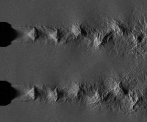
The coupling behaviour is dependent on the nozzle spacing between the two jets,  $s/D$, and Mach number (Knast et al. Reference Knast, Bell, Wong, Leb, Soria, Honnery and Edgington-Mitchell2018), which in a purely converging nozzle is dependent only on the nozzle pressure ratio (NPR). The two examples of coupling symmetries in the parallel $y$ plane are provided in figure 1, which shows schlieren snapshots at $s/D = 2,\ {\rm NPR} = 3.86$ and $s/D=4,\ {\rm NPR} = 3.86$. Here $s$ is the distance between the nozzle centres, $D$ is the nozzle inner diameter, and NPR is the ratio between the ambient pressure at the exhaust to the stagnation pressure at the nozzle exit (Raman et al. Reference Raman, Panickar and Chelliah2012). Both SS and SA coupling of $m=1$ equivalent modes in a twin-axisymmetric-jet system are observed at these conditions.

Figure 1. Schlieren image of (a)  $s/D = 2$, ${\rm NPR} = 3.86$ SS and (b) $s/D = 4$, ${\rm NPR} = 3.86$ SA coupling. Knife-edge oriented such that the density fluctuations in the streamwise direction are captured.
The resonance that occurs in twin-jet systems is both of significantly higher amplitude than that observed in isolated jets and also appears to be more prevalent in full-scale engines; while screech in isolated jets seldom occurs outside the laboratory, fatigue-induced failure associated with screech in twin jets has been observed in a number of aircrafts (Berndt Reference Berndt1984). The flapping mode in a twin-jet system appears to be more strongly amplified than the axisymmetric mode (Kuo, Cluts & Samimy Reference Kuo, Cluts and Samimy2017). Knast et al. (Reference Knast, Bell, Wong, Leb, Soria, Honnery and Edgington-Mitchell2018) used schlieren data from two perspectives to investigate the relationship between operating condition, coupling symmetry and the azimuthal modes of twin round jets. While the interpretation of some operating conditions was difficult due to the limitations of the experimental technique, the authors nonetheless demonstrated that twin-jet systems both experience modal staging in a manner reminiscent of an isolated jet, but can also undergo changes in symmetry not associated with a discontinuous change in frequency. Some of the modal staging was associated with a change in the match between the wavelengths of the shock and the standing wave, which are now known to indicate changes in the region of the quasi-periodic shock structure that is generating the guided-jet mode (Edgington-Mitchell et al. Reference Edgington-Mitchell, Li, Liu, He, Wong, Mackenzie and Nogueira2022). However, some modal staging behaviour was not explicable via this mechanism, suggesting additional physics at play in the twin-jet system.
1.3. Screech in twin non-circular jets
The screech phenomenon is not limited to twin round jets but is also observed in twin rectangular jets (Raman & Taghavi Reference Raman and Taghavi1998; Jeun, Wu & Lele Reference Jeun, Wu and Lele2020; Karnam, Baier & Gutmark Reference Karnam, Baier and Gutmark2020; Ghassemi Isfahani, Webb & Samimy Reference Ghassemi Isfahani, Webb and Samimy2021a; Jeun et al. Reference Jeun, Karnam, Jun Wu, Lele, Baier and Gutmark2022). Akin to round jets, symmetric coupling between rectangular jets produces maximum pressure in the internozzle region, whereas antisymmetric coupling produces minimum pressure (Raman & Taghavi Reference Raman and Taghavi1998). The coupling behaviour of rectangular twin jets, similar to round jets, is a function of both nozzle spacing and NPR. From a study conducted by Raman & Taghavi (Reference Raman and Taghavi1998), mode switching was characterised through a parameter  $\alpha$, which determined a ‘null’ phase region where the two jets overlapped or did not. When separate, antisymmetric coupling occurred and if the ‘null’ region overlapped then jets coupled symmetrically. Moreover, the transition from antisymmetric to symmetric coupling leads to a transition of the effective sound source location from the third shock cell to the fourth shock cell. The turbulence levels in the shear layer vary depending on the mode of the rectangular jets; a flapping mode induced by screech led to higher turbulence levels in the inner shear layers due to a large dissipation rate caused by the flapping motion (Karnam et al. Reference Karnam, Baier and Gutmark2020).
1.4. Intermittency in the coupling of twin-jet systems
At specific nozzle spacings and Mach numbers, the coupling behaviour can become erratic, leading to periods where the jet can switch between symmetric or antisymmetric modes or uncouple entirely (Bell et al. Reference Bell, Cluts, Samimy, Soria and Edgington-Mitchell2021). This has been suggested to be the result of a competition between global modes of the flow, which is supported by the fact that different coupling symmetries exhibit similar growth rates and wavenumbers for the Kelvin–Helmholtz instability (Nogueira & Edgington-Mitchell Reference Nogueira and Edgington-Mitchell2021). The development of better experimental and high-fidelity numerical tools has facilitated the quantification of intermittency in a number of jet flows, including subsonic (Grizzi & Camussi Reference Grizzi and Camussi2012) and supersonic regimes (Sasidharan Nair, Agostini & Gaitonde Reference Sasidharan Nair, Agostini and Gaitonde2015; Meloni & Jawahar Reference Meloni and Jawahar2022). In these isolated jets intermittency is characterised either by interruptions in near-field pressure fluctuations or far-field noise. For twin jets and the processes involved in each jet, interruptions in the coupling between the jets provide an additional mechanism for intermittency. The aforementioned study by Bell et al. (Reference Bell, Cluts, Samimy, Soria and Edgington-Mitchell2021) on twin round jets used modal decomposition of particle image velocimetry (PIV) data alongside time-frequency analysis of acoustic data to demonstrate that at some operating conditions the coupling between jets was steady, and at other conditions was highly intermittent. In rectangular twin jets intermittency has been observed both experimentally (Ghassemi Isfahani, Webb & Samimy Reference Ghassemi Isfahani, Webb and Samimy2021b) and numerically (Jeun, Wu & Lele Reference Jeun, Wu and Lele2021a; Jeun et al. Reference Jeun, Karnam, Jun Wu, Lele, Baier and Gutmark2022). In these studies, the nozzle was converging–diverging, and different degrees of intermittency were observed depending on whether the jets were in the overexpanded or underexpanded state. It is important to note that twin jets, like other resonant aeroacoustic systems, are characterised by a high degree of facility sensitivity. In the aforementioned studies on rectangular jets, though both systems were intermittent, the nature of the intermittency was qualitatively different. In Bell et al. (Reference Bell, Cluts, Samimy, Soria and Edgington-Mitchell2021) similar round nozzles were studied in two facilities; while both facilities produced identifiable regions of steady and unsteady coupling, the transitions between these regions occurred at different NPR values. The results of any study of resonant coupling between twin jets will thus be specific to the boundary conditions of the simulation or experiment in question. What is clear from the extant literature, however, is that intermittency in these systems appears to be a general phenomenon. The exact mechanism underpinning intermittency in twin-jet systems remains unclear; both Bell et al. (Reference Bell, Cluts, Samimy, Soria and Edgington-Mitchell2021) and Jeun et al. (Reference Jeun, Wu and Lele2021a) suggested a competition between global modes of the flow associated with different symmetries. Jeun et al. (Reference Jeun, Wu and Lele2021a) suggested that this competition might manifest as a competition between different resonances; self-excitation by individual jets as opposed to cross-excitation between the jets.
1.5. Modal decomposition techniques for the study of intermittency
Educing the coupling mode of the jets typically requires some form of modal decomposition, such as proper orthogonal decomposition (POD, Sirovich Reference Sirovich1987) or its spectral form (SPOD, Lumley Reference Lumley1967; Towne, Schmidt & Colonius Reference Towne, Schmidt and Colonius2018). Bell et al. (Reference Bell, Cluts, Samimy, Soria and Edgington-Mitchell2021) employed POD on PIV data when investigating two different operating conditions in twin round jets:  $s/D=3$, ${\rm NPR}=4.6$ and 5.0. For ${\rm NPR}=5.0$, a symmetric coupling signature was observed in the POD spatial modes. A difficulty arose for the unsteady, intermittent ${\rm NPR} = 4.6$ case, where the application of POD, without any transformations to the data, led to POD modes with a $90^\circ$ offset between the two jet plumes and no clear evidence of a modal pair representing a travelling wave structure (Taira et al. Reference Taira, Brunton, Dawson, Rowley, Colonius, McKeon, Schmidt, Gordeyev, Theofilis and Ukeiley2017). By subsectioning the top and bottom plumes and applying POD on conditionally sampled data, the authors were able to demonstrate that the jet has periods where neither, one or both jets are oscillating. A limitation in Bell et al. (Reference Bell, Cluts, Samimy, Soria and Edgington-Mitchell2021) was that the PIV data were not time resolved, leading to the inability to visualise the precise temporal behaviour of the jets – whether they are uncoupled, coupled or switching between coupling. Time-resolved data are amenable to a range of further decomposition techniques that can provide information regarding the time-varying behaviour of the flow, which is critical when quantifying intermittency. Sasidharan Nair et al. (Reference Sasidharan Nair, Agostini and Gaitonde2015) used short-time Fourier transforms and empirical-mode decomposition to investigate the intermittency of wavepackets in the near field of a supersonic jet. Wavelet analysis offers a robust means of quantifying intermittency and is increasingly used in the study of high-speed jets (Grizzi & Camussi Reference Grizzi and Camussi2012; Jeun et al. Reference Jeun, Wu and Lele2021a, Reference Jeun, Karnam, Jun Wu, Lele, Baier and Gutmark2022; Meloni & Jawahar Reference Meloni and Jawahar2022).
1.6. Summary
In the work of Bell et al. (Reference Bell, Cluts, Samimy, Soria and Edgington-Mitchell2021), our group investigated coupling intermittency in the highly underexpanded regime, at  ${\rm NPR} = 4.6$ and ${\rm NPR} = 5.0$. At the higher Mach numbers associated with these pressures, the jets are characterised by $m=1$ azimuthal modes, resulting in four possible coupling symmetries (Morris Reference Morris1990). At lower Mach numbers, the jets screech in the $m=0$ mode, which reduces the number of possible coupling symmetries to two (Stavropoulos et al. Reference Stavropoulos, Mancinelli, Jordan, Jaunet, Edgington-Mitchell and Nogueira2021), which are easy to differentiate between using flow visualisation. As correctly identifying the coupling symmetry (or lack thereof) is critical to our assessment of intermittency, in this work we restrict our attention to the Mach numbers associated with the A1 and A2 branches of jet screech in the low supersonic regime. The assessment of intermittency in Bell et al. (Reference Bell, Cluts, Samimy, Soria and Edgington-Mitchell2021) relied on acoustic measurements and non-time-resolved PIV data, here we extend this approach through the application of time-frequency analysis to high-speed schlieren data for twin round jet systems. A combination of POD, SPOD and wavelet analysis is applied to visualisations of twin jets operating at a range of internozzle spacings and NPRs. The paper is set out as follows. Section 2 will outline the experimental twin-jet set-up and, in § 3, the analysis tools used to characterise the coupling behaviour. Section 4 presents an overview of the parameter space studied before providing a deeper examination of several possible coupling states: steady coupling, competitive coupling and unsteady coupling. Lastly, § 5 summarises the key findings of the paper.
2. Experimental set-up
Experiments were undertaken at the Laboratory for Turbulence Research in Aerospace and Combustion (LTRAC) at Monash University. The laboratory is temperature controlled with temperature fluctuations of the order of 0.1 K across the three days; such fluctuations in temperature and humidity can be expected to not affect measurements. The experimental set-up is similar to that described in Knast et al. (Reference Knast, Bell, Wong, Leb, Soria, Honnery and Edgington-Mitchell2018), and the reader is referred to that study for details of the design. The supersonic twin jets are imaged using a Toepler Z-Type schlieren system using twin parabolic mirrors, each with a focal length of 2032 mm (Settles Reference Settles2001). Illumination is provided via pulsed LED (Willert, Mitchell & Soria Reference Willert, Mitchell and Soria2012) with a pulse width of 1  $\mathrm {\mu }$s. The data are collected on a Photron FASTCAM SA-Z 2100 K camera. The experimental set-up and coordinate planes are defined in figure 2. A high-pressure air supply accelerates the jets to the supersonic regime. Prior to entry into the plenum chamber, the flow passes through a regulator and the stagnation pressure is measured in the plenum using an RS-461 pressure transducer. Both jets share the same plenum. The transducer is rated to have a range of 0 $-$10 bars with an accuracy of ${\pm }0.25\,\%$. Only path-integrated streamwise density fluctuations ( ${\partial \rho }/{\partial x}$) will be presented, and pictures are taken only in the ( $x,y$) plane (see figures 2(a) and 2(b)) – and thereby only one plane of the twin-jet coupling corresponding to SS and SA symmetries will be presented. We refer to the jets in the positive and negative $y$ half-planes as the top and bottom jets, respectively. A parameter sweep was performed at nozzle spacings of $s/D = 2, 3, 4$ and 6 at an NPR ranging from 2.02 to 2.41 – covering the A1 and A2 screech frequency branches in increments of approximately 0.05 NPR. To capture $s/D=6$ within the imaging frame, a $384\times 384$ resolution was used compared with the $256\times 384$ resolution for the other spacings. This change in resolution also meant that $s/D=2$, 3 and 4 were taken at an acquisition speed of 150 000 Hz, whereas for $s/D=6$, it was 100 000 Hz. Frequency is non-dimensionalised as Strouhal number, $St={fD}/{U_j}$, where $f$ is the frequency and $U_j$ is the ideally expanded jet velocity. When applicable, time is non-dimensionalised by the screech period based on the top jet, $t^*=tf_t$, where $t$ is the time of the recording in seconds and $f_t$ is the fundamental screech tone of the top jet. The choice of jet whose screech frequency is used to define $t^*$ is arbitrary, but the differences between the two jets are small enough not to impact the interpretation of the results.

Figure 2. Twin-jet configuration in  $(x,y)$ plane (a), experimental set-up (b) and internal geometry of nozzles, with dimensions given in millimetres (c).
3. Analysis techniques
An ensemble of data decomposition techniques is used to determine potential temporal symmetric and antisymmetric switching in the jet as well as the duration for which the jets uncouple. Each technique will be briefly reviewed in this section.
3.1. Proper orthogonal decomposition
Proper orthogonal decomposition decomposes the flow field into optimally energy-ranked spatially coherent modes. Proper orthogonal decomposition has been applied across a wide range of fields, and it has been especially effective in extracting the coherent structures in screeching jets (Berry, Magstadt & Glauser Reference Berry, Magstadt and Glauser2017; Bell et al. Reference Bell, Cluts, Samimy, Soria and Edgington-Mitchell2021; Edgington-Mitchell et al. Reference Edgington-Mitchell, Wang, Nogueira, Schmidt, Jaunet, Duke, Jordan and Towne2021; Nogueira & Edgington-Mitchell Reference Nogueira and Edgington-Mitchell2021). First introduced by Lumley (Reference Lumley1967) and popularised in its standard form by Sirovich (Reference Sirovich1987), POD formulates its mean subtracted flow field as
 \begin{equation} \boldsymbol{q}(\boldsymbol{x} ,t)-\boldsymbol{\bar{q}}(\boldsymbol{x}) = \sum_{j}a_j(t)\boldsymbol{\phi}_j(\boldsymbol{x}), \end{equation}
where  $\boldsymbol {\phi _j}$ are the spatial modes and $a_j(t)$ are their respective temporal coefficients. The POD modes are obtained here using the method of snapshots (Sirovich Reference Sirovich1987) via
 \begin{gather} \boldsymbol{\mathsf{Q}}^{\rm T}\boldsymbol{\mathsf{Q}}\boldsymbol{\psi}_j=\lambda_j\boldsymbol{\psi}_j, \end{gather}
 \begin{gather}\boldsymbol{\phi}_j=\boldsymbol{\mathsf{Q}}\boldsymbol{\psi}_j\frac{1}{\sqrt{\lambda_j}}, \end{gather}
where  $\boldsymbol{\mathsf{Q}}=[\boldsymbol {q}_1,\boldsymbol {q}_2,\ldots,\boldsymbol {q}_N]$ and $q$ contain the light intensities of the snapshot and is acting as a proxy for path-integrated density fluctuations – across all space and time. Here $\lambda _j$ is the modal energy of the $j$th mode.
3.2. Spectral POD
Spectral POD is a modal decomposition technique that extracts frequency-dependent spatially coherent modes of the flow, assuming that the flow data are statically stationary (Lumley Reference Lumley1967; Glauser, Leib & George Reference Glauser, Leib and George1987; Delville et al. Reference Delville, Ukeiley, Cordier, Bonnet and Glauser1999; Gordeyev & Thomas Reference Gordeyev and Thomas2000; Towne et al. Reference Towne, Schmidt and Colonius2018). Spectral POD has seen numerous applications in many flow fields where it is pertinent to extract out the spatial modes of large coherent structures at a certain frequency (Schmidt et al. Reference Schmidt, Towne, Rigas, Colonius and Brès2018; Sano et al. Reference Sano, Abreu, Cavalieri and Wolf2019; Ghate, Towne & Lele Reference Ghate, Towne and Lele2020; Jeun et al. Reference Jeun, Wu, Lele, Karnam, Baier and Gutmark2021b; Morra et al. Reference Morra, Nogueira, Cavalieri and Henningson2021; Nekkanti & Schmidt Reference Nekkanti and Schmidt2021). The SPOD modes are defined in terms of the eigenvalue problem
 \begin{equation} \hat{\boldsymbol{\mathsf{C}}}\boldsymbol{\mathsf{W}}\hat{\boldsymbol{\phi}}= \hat{\boldsymbol{\phi}}\hat{\varLambda}, \end{equation}
where  $\hat {\boldsymbol{\mathsf{C}}}$ is the cross-spectral density matrix, $\hat {\boldsymbol {\phi }}$ is the matrix containing the SPOD modes, $\hat {\varLambda }$ is the diagonal modal energy matrix and $\boldsymbol{\mathsf{W}}$ is a weight matrix that defines the norm in which the modes are optimal. The reader is referred to Schmidt & Colonius (Reference Schmidt and Colonius2020) for further details on SPOD. All SPOD results were generated using a uniform weighting matrix, Hanning window, 50 % overlap and $N_{FFT}=4800$ unless stated otherwise. Due to the difference in image resolution between $s/D=2,3,4$ and $s/D=6$, as well as computational limitations, $N= 50\,000$ is used for the former spacings and $N=40\,000$ is used for the latter, where $N$ denotes the number of schlieren snapshots.
3.3. Continuous wavelet transform
Time-frequency information is extracted via the continuous wavelet transform (CWT) (Farge Reference Farge1992). The CWT convolves a given signal with a wavelet across a range of scales, a, and time shifts, b, to yield a wavelet coefficient,
 \begin{equation} T(a,b)=\frac{1}{\sqrt{a}}\int_{-\infty}^{\infty}q(t)\psi^*\left(\frac{t-b}{a}\right){\rm d} t, \end{equation}
where  $q$ represents the signal and $\psi$ is a chosen mother wavelet that is shifted and dilated across the signal. The scales provide the frequency information about the signal, and the time shift yields the temporal information. A complex Morlet wavelet
 \begin{equation} \psi_m(t)=\frac{1}{B_c\sqrt{2{\rm \pi}}}\exp\left({-\frac{t^2}{2B_c^2}}\right) \exp({j2{\rm \pi} f_ct}),\quad B_c=\frac{c}{k_{sd}f_c}, \end{equation}
is chosen as the mother wavelet for the purpose of twin-jet analysis due to its suitability for fluids in general (Li et al. Reference Li, Liu, Xing and Guo2018). Here  $f_c$ is the central frequency, $B_c$ is the time spread parameter, $c$ is the number of cycles of the wavelet and $k_{sd}$ is the standard deviations of the Gaussian envelope. The standard deviation $k_{sd}$ is chosen to be 5, a suitable design choice for analyses of this type (Moca et al. Reference Moca, Bârzan, Nagy-Dăbâcan and Mureşan2021). As wavelet coefficients are complex, they are often analysed in terms of their time and scale-dependent power,
 \begin{equation} P(a,b)=T(a,b)\times T^*(a,b)=|T(a,b)|^2. \end{equation}
The power is then typically visualised on a scalogram, i.e. contours of  $P(a,b)$ as a function of time and frequency. For our study of twin jets, large values of $P(a,b)$ indicate a large resonance amplitude at the given time and frequency. Frequency can be recovered from the scale using the relation $a = f_c / f$.
The CWT is useful because the system is intermittent, and the transform can identify periods during which the jet resides in each state. A notable parameter is the number of cycles,  $c$, which can be varied to achieve the desired frequency resolution, with a larger $c$ corresponding to a finer resolution. However, higher frequency resolution leads to lower temporal resolution as dictated by the Heisenberg–Gabor uncertainty principle (Gabor Reference Gabor1946), which states that if there is precise certainty of when a wave is localised in time, there is a resulting compromise in large uncertainty in its frequency.
Therefore, if the twin-jet system is rapidly switching between two close frequencies, CWT will not be able to properly resolve the frequencies. Nonetheless, our results indicate that adequate time-frequency localisation is obtained through the appropriate use of a high frequency resolution ( $c=600$) and high temporal resolution ( $c=3$).
3.4. Exploiting symmetries
Although significant information can be gleaned from the application of these analysis techniques on the mean-subtracted schlieren snapshots, further insight can be extracted through a preliminary transformation of the snapshots. Two such transforms are considered. First, each snapshot can be segregated into two halves, isolating the top and bottom jets. This can be mathematically expressed as
 \begin{gather} \boldsymbol{\mathsf{Q}}_{\boldsymbol{\mathsf{t}}}(x,y) = \boldsymbol{\mathsf{Q}}(x,y),\quad \textrm{where}\ y\in T, \end{gather}
 \begin{gather}\boldsymbol{\mathsf{Q}}_{\boldsymbol{\mathsf{b}}}(x,y) = \boldsymbol{\mathsf{Q}}(x,y),\quad \textrm{where}\ y \in B, \end{gather}
where  $\boldsymbol{\mathsf{Q}}_{\boldsymbol{\mathsf{t}}}$ and $\boldsymbol{\mathsf{Q}}_{\boldsymbol{\mathsf{b}}}$ represent the light intensities of only the top and bottom jets, respectively, and $T$ and $B$ are sets that only include the top and bottom half of the light intensities of a snapshot (see figure 2a). This transformation aims to keep only one jet in the frame for a given snapshot so that analysis can be conducted either on the top or bottom jet only. Therefore, from this half-domain (HD) transform, one jet can be focused on at a time, allowing for the extraction of similarities and differences in the behaviour of each jet.
Second, the top–bottom symmetry of the physical set-up can be imposed on the data. Symmetry imposition (SI) follows Nogueira & Edgington-Mitchell (Reference Nogueira and Edgington-Mitchell2021) whereby the schlieren light intensity data are transformed into snapshots that only show potential symmetric,  $\boldsymbol{\mathsf{Q}}_{\boldsymbol{\mathsf{e}}}$, or antisymmetric, $\boldsymbol{\mathsf{Q}}_{\boldsymbol{\mathsf{o}}}$, coupling.
 \begin{gather} \boldsymbol{\mathsf{Q}}_{\boldsymbol{\mathsf{e}}}(x,y)= \frac{\boldsymbol{\mathsf{Q}}(x,y)+\boldsymbol{\mathsf{Q}}(x,-y)}{2}, \end{gather}
 \begin{gather}\boldsymbol{\mathsf{Q}}_{\boldsymbol{\mathsf{o}}}(x,y)=\frac{\boldsymbol{\mathsf{Q}}(x,y)- \boldsymbol{\mathsf{Q}}(x,-y)}{2}. \end{gather}
If no transformation is applied, that will be referred to as full domain (FD) snapshots.
Direct application of CWT on the raw schlieren data often leads to noisy and unintelligible scalograms, hindering any useful insight into the temporal-frequency behaviour of the twin jet. However, this can be overcome by leveraging POD's strength as a noise-filtering algorithm. Proper orthogonal decomposition has similar capabilities to SPOD as both are based on spatial correlations of the coherent structures in the flow field. Moreover, POD output temporal coefficients combined with time-frequency analysis through wavelets form a powerful combination to glean key insights into twin-jet behaviour. Although the POD modes are computed via an ensemble average across the snapshots, these temporal coefficients are instantaneous quantities that can be used to understand when the structures are active in the flow. In this framework, the most energetic modes will be given as input for CWT to denoise the scalogram and gain insight into the temporal-frequency information of coherent structures in the twin jet. Moreover, the application of the aforementioned data decomposition techniques on the transformed data allows for extensive mapping of the behaviour of the twin-jet system in the temporal, frequency and spatial domains. For instance, applying a HD transformation before applying POD and CWT on the temporal coefficients (scaled by its respective modal energy) can determine how the fundamental frequency of each jet varies across time. This is visualised by the wavelet power
 \begin{equation} P_{j_{HD}}=|T_{j_{HD}}|^2,\quad T_{j_{HD}}=\frac{1}{\sqrt{a}} \int_{-\infty}^{\infty} \lambda_{j_{HD}} a_{j_{HD}}\psi^*\left(\frac{t-b}{a}\right){\rm d} t, \end{equation}
where  $T_{j_{HD}}$ and $P_{j_{HD}}$ are the wavelet coefficient and power, respectively, for the $j$th mode and $a_{j_{HD}}$ is the associated temporal coefficients in the HD. The HD denotes either the top or bottom jet. Proper orthogonal decomposition typically decomposes the jet flow in mode pairs for jet screech as there are a small number of very dominant waves. These mode pairs form a travelling wave; therefore, a more appropriate wavelet power to plot would be the sum of the wavelet powers of the two modes in a pair. However, proper identification of the mode pairs can prove difficult for some cases, as seen in § 4 and in Appendix B. Moreover, the summation of mode pairs leads to negligible differences in the scalogram. Instead, all scalograms in this paper correspond to the temporal coefficients of the leading POD mode.
An expression analogous to (3.12) can be written for the SI temporal coefficients,  $a_{j_{SI}}$, to allow for visualization of which symmetries are dominant over a given period. Lastly, although an HD or SI transformation can be applied before SPOD is conducted, much of that information is already elucidated by CWT on the POD temporal coefficients. Therefore, standard SPOD will be applied to the FD schlieren data to extract the modal energy and spatial modes of the flow field. A summary of the relevant techniques applied to the twin-jet data, along with their use cases and limitations, are provided in table 1.
Table 1. Data decomposition techniques applied on the twin-jet system

4. Results
4.1. Coupling behaviour across the parameter space
A survey of the resonant frequency of the twin-jet system is produced by computing the SPOD spectra of the optimal mode across the parameter space, shown in figure 3. Quantification of SS- and SA-dominated conditions are outlined in Appendix A. For the sake of comparison, the SPOD spectra for a single jet are also provided in figure 3(a). For details of the single-jet data, the reader is referred to the Monash University dataset in Edgington-Mitchell et al. (Reference Edgington-Mitchell, Li, Liu, He, Wong, Mackenzie and Nogueira2022). The peak frequencies across all twin-jet spacings are similar, with screech beginning at  ${\rm NPR}=2.07$ with the A1 acoustic branch spanning to ${\rm NPR} = 2.17$ and the A2 acoustic branch spanning ${\rm NPR}=2.22$ to $2.36$. For the twin jet, modal staging between A1 and A2 occurs from ${\rm NPR} = 2.17$ to $2.22$, and the A2 to B staging is present at the ${\rm NPR} = 2.31$ and $2.36$ region, with some spacings featuring the presence of both frequencies at these NPRs. This is the same behaviour as observed in the single jet, though at ${\rm NPR} = 2.1$, there is more evidence of competition between the A1 and A2 modes for the single jet. This result is consistent with the acoustic data presented in Knast et al. (Reference Knast, Bell, Wong, Leb, Soria, Honnery and Edgington-Mitchell2018), who also observed that the A1-A2-B modal staging was similar in twin and single jets.

Figure 3. Spectra associated with the first SPOD mode from schlieren images as well as coupling states for  $s/D=2,3,4$ and $6$. Purple and red points indicate a relatively strong SA and SS symmetry, respectively. Black indicates either the same strength in SS and SA or uncoupling. (a) Single jet; (b) $s/D=2$; (c) $s/D=3$; (d) $s/D=4$; (e) $s/D=6$.
Some additional features are evident in the twin-jet configuration at the operating conditions where transitions between modal stages occur. For instance, dual peaks associated with the A2 mode are evident for  $s/D=6$ at ${\rm NPR} = 2.22$ and $2.36$. It will be demonstrated in § 4.3 that this is indicative that the jets have uncoupled from each other at these conditions. Though not clearly demarcated as individual peaks, the broad peak associated with the B mode at ${\rm NPR} = 2.36$ for $s/D = 2,3$ is likely indicative of similar physics.
Figure 3 also surveys the various coupling and symmetry states of the twin-jet system. Each condition is characterised by two parameters: the steadiness of the coupling and the relative strength of the symmetries. When the coupling is steady, it is associated with a single symmetry. In the cases where there is competition or switching between symmetries, one symmetry may still be relatively dominant, or the system may exhibit no strong preference for either SS or SA symmetry. As alluded to earlier, an additional possibility is that the jets can uncouple, in which case they no longer exhibit symmetry. As well as competition between symmetries, for operating conditions where modal staging transitions occur, there can also be competition between the A1/A2/B branches. These have been studied previously for single jets (Mancinelli et al. Reference Mancinelli, Jaunet, Jordan and Towne2019), but in the present work are omitted for brevity.
As is evident in figure 3, a broad range of behaviours are observed even in this relatively constrained parameter space. For example, at a single spacing of  $s/D=3$, there are four distinct forms of coupling observed over the six data points studied. In the A2 branch, steady coupling is observed for each operating condition, but the dominant symmetry switches between SS and SA. An exemplar of this steady coupling is explored in § 4.2. At ${\rm NPR} = 2.07$, there is evidence of competition between the symmetries, but the SA symmetry manifests significantly more often. By ${\rm NPR} = 2.12$, this preference for SA symmetry is no longer apparent, and the system is switching between the two states on relatively short time scales; competition between symmetries of this kind is explored in § 4.4. There are also the aforementioned conditions at $s/D=6$ where the jets uncouple. This uncoupling can take the form of intermittency, such as at ${\rm NPR} = 2.26$, where the red symbol diamond indicates that there is competition between the SS symmetry and an uncoupled state; coupling of this kind is discussed further in § 4.5. Finally, the jets can entirely uncouple, as evident at ${\rm NPR} = 2.22$, as discussed in § 4.3.
Some trends with NPR are apparent across all spacings. In the early part of the A1 branch ( ${\rm NPR}=2.07$ and $2.12$), there is competition between symmetries, though the system nonetheless generally exhibits a preference for the SA symmetry at five out of the eight data points considered. The first exception is at $s/D=3, {\rm NPR} = 2.12$, where the system switches between SS and SA in roughly equal measure. The other exception is at $s/D = 4,\ {\rm NPR} = 2.07$, where there is still competition, but with the SS symmetry appearing dominant. At ${\rm NPR} = 2.17$, the dominant symmetry is less clear; SA at $s/D=2$, SS for $s/D = 3,6$ and no clear dominance for $s/D = 4$.
In the A2 branch  $2.22 \leq {\rm NPR} \leq 2.36$, the dominant symmetry switches to SS; seven of the ten data points classified in the A2 branches correspond to an SS symmetry. The exceptions are at $s/D=3$, where two of the conditions demonstrate steady SA coupling, and the first point of the A2 branch for $s/D=6$, where the jets uncouple completely. As will be demonstrated in § 4.3, the jets are not truly identical; manufacturing tolerances result in a disparity of 0.03 % in the fundamental screech tone of each jet. However, at most operating conditions explored in this paper, the jets are observed to couple together, and the system closely approximates symmetry within the precision of the schlieren visualizations. The degree of unsteadiness is also dependent on $s/D$; the least unsteadiness is observed for the A2 branch at the closer spacings ( $s/D=2$ and $3$), the most unsteadiness is observed for $s/D=6$. Even at $s/D=6$, steady coupling is still evident in the SS symmetry at two data points, though at several other operating conditions, the jets exhibit intermittent or total uncoupling. It should be emphasised that the classifications presented here are for recordings of length $t=0.5$ s; there may be low frequency variation in the supply pressure, or other external effects, which are not captured in the present analysis. However, this record length represents $O(10^3)$ screech cycles and, thus, should accurately represent processes in the jets themselves.
The A1-to-A2 modal staging appears to have a strong effect on the coupling state; all four spacings exhibit some change in the dominant coupling symmetry when the mode transition occurs. Here  $s/D = 2$ switches from SA to SS coupling, $s/D = 3$ exhibits the opposite effect and switches from SS to SA instead. Modal staging results in the jets uncoupling, rather than switching symmetries, for $s/D = 6$. The final data point on the A2 branch for $s/D = 2$ and $s/D = 4$ exhibited intermittent switching between the A2 and B modes; as the focus of this work is on the $m=0$ modes, no further classification of these data was attempted.
With the overview of the parameter space completed, we will now undertake a more detailed discussion of a range of exemplar cases. Examination of these exemplar cases is intended to demonstrate the various forms that intermittency might take in a twin-jet system, as well as to clarify the interpretation of the various analysis techniques mentioned in § 3. However, due to facility sensitivity, we do not suggest that the behaviours observed here would be exactly replicated in another experiment; we expect any facility will exhibit regions of steady or unsteady coupling as a function of nozzle separation and operating condition, but the specific values will depend on the boundary conditions of the experiment. In producing figure 3 we have, of necessity, compressed a great deal of complexity into a small number of categories. But in the following sections we will not only explore the differences between the various categories identified thus far but also differentiate between cases in nominally the same category, based on degree and frequency of intermittency.
4.2. Steady coupled jets
At some operating conditions, the twin-jet system presents steady behaviour, locking to a single symmetry for the length of the observation period. Interpretation of the modal decomposition techniques at these steady coupling conditions is relatively straightforward, so these conditions are a logical starting point for discussion. One such case where SA coupling dominates is  $s/D=2$, ${\rm NPR}=2.17$. To begin analysis on the coherent structures of the twin jet at this condition, POD is applied on the HD ( $\boldsymbol{\mathsf{Q}}_{\boldsymbol{\mathsf{t}}}$ and $\boldsymbol{\mathsf{Q}}_{\boldsymbol{\mathsf{b}}}$) and symmetry imposed ( $\boldsymbol{\mathsf{Q}}_{\boldsymbol{\mathsf{e}}}$ and $\boldsymbol{\mathsf{Q}}_{\boldsymbol{\mathsf{o}}}$) fields; the modal energies, temporal coefficients and spatial structure of the leading POD modes are shown in figure 4. For a more in-depth discussion of the POD analysis for this case and subsequent operating conditions, the reader is referred to Appendix B. For the modal energies presented in figure 4, the ordinate axis represents the percentage energy contribution of the top and bottom jets for HD and even and odd transformations for SI. It must be noted that POD (and SPOD) ‘energy’ is not clearly defined, being based on light intensity acting as a proxy for the path-integrated density-gradient fluctuations. Absolute values of energy are essentially meaningless, as is comparing energies between different cases; however, the technique is nonetheless robust for identifying structures in screeching jets. Two leading modes are evident in the top and bottom jet and odd fields, indicative of structures associated with a single resonant process at a fixed frequency. Comparison between the top and bottom jet mode energies shows that the fluctuations in the two jets are of similar amplitude. At this condition, the jets exhibit an SA symmetry, demonstrated by the disparity between even and odd SI modal energies; there is a leading modal pair for the odd decomposition and none for even. The temporal coefficients of the leading POD mode are given in figures 4(b) and 4(d) for the first 15 screech cycles. These temporal coefficients echo the same conclusions suggested by the modal energy distribution through inspection of the relative amplitudes; that there is a similar resonance between the two jets and dominance in SA coupling. Visual confirmation is shown through the presence of both jets in an SA configuration in the spatial structure of the leading POD mode pair (figures 4(e) and 4(f)). While the two POD analyses presented thus far suggest a strong preference for SA coupling, time-frequency analysis can provide a more robust data interrogation.

Figure 4. The POD modal energy of  $\boldsymbol{\mathsf{Q}}_{\boldsymbol{\mathsf{t}}}$ and $\boldsymbol{\mathsf{Q}}_{\boldsymbol{\mathsf{b}}}$ (a); $\boldsymbol{\mathsf{Q}}_{\boldsymbol{\mathsf{e}}}$ and $\boldsymbol{\mathsf{Q}}_{\boldsymbol{\mathsf{o}}}$ (b). Temporal coefficients of $\boldsymbol{\mathsf{Q}}_{\boldsymbol{\mathsf{t}}}$ and $\boldsymbol{\mathsf{Q}}_{\boldsymbol{\mathsf{b}}}$ (c); $\boldsymbol{\mathsf{Q}}_{\boldsymbol{\mathsf{e}}}$ and $\boldsymbol{\mathsf{Q}}_{\boldsymbol{\mathsf{o}}}$ (d). Spatial structure of modes 1 (e) and 2 (f) of $\boldsymbol{\mathsf{Q}}_{\boldsymbol{\mathsf{FD}}}$. The system is operating at $s/D = 2$, ${\rm NPR}=2.17$.
The time-frequency information is extracted by performing CWT on the temporal coefficients, yielding the HD-POD-CWT and SI-POD-CWT scalograms shown in figure 5. Figures 5(b) and 5(c) show the scalograms for HD-POD-CWT, that is, for the top and bottom jet, respectively. The abscissa denotes the number of screech cycles, the ordinate axis shows  $St$ and the contour level indicates the wavelet power. In a configuration where the twin-jet system is strongly coupled, the scalograms for the top and bottom jets should be very similar; this is evident in figures 5(b) and 5(c) and corroborates the POD modal energy distribution in the HD field. Here, each jet is screeching at the same frequency, which varies slightly across time. The small difference in wavelet power between the two jets could be due to imperfections in the optical set-up: uneven focus or illumination in different parts of the domain. Figure 5(a) represents the scalogram of the SI field, $\boldsymbol{\mathsf{P}}_{\boldsymbol{\mathsf{1}}_{\boldsymbol{\mathsf{e}}}}$ and $\boldsymbol{\mathsf{P}}_{\boldsymbol{\mathsf{1}}_{\boldsymbol{\mathsf{o}}}}$, with the even and odd power separated by contour colour. The relative strength of each power indicates whether the system is coupled in an SS or SA manner. Cases featuring a dominant single symmetry are characterised by a strong resonance in either even or odd scalograms but not both; typically, the power in the dominant symmetry is at least an order of magnitude higher than its counterpart. The present case is one such example, with the antisymmetric coupling (SA) dominant over the entire time series. The band at $St = 0.636$ in all scalograms indicates that the twin-jet system is resonating at the aforementioned frequency, and small fluctuations in frequency are likely due to fluctuations in supply pressure. The weak wavelet power in the even scalogram aligns well with the low modal energy seen in figure 4(c), reinforcing the notion that there is an absence of SS coupling at this condition.

Figure 5. Scalograms of  $\boldsymbol{\mathsf{P}}_{\boldsymbol{\mathsf{1}}}$ for SI (a), top jet (b) and bottom jet (c) fields. The system is operating at $s/D = 2$, ${\rm NPR}=2.17$.
In summary, the similarity between the HD analyses indicates that the jets are always coupled, and the relative power of the symmetry-enforced analyses indicates that this coupling is of the SA family.
The previous analyses only considered half the domain, whether by omission or symmetry enforcement. An assessment of the spatio-temporal structure of the entire domain is best performed using SPOD. The optimal SPOD mode,  $\boldsymbol {\varLambda _{1}}$, shown in figure 6(b), indicates an antisymmetric coupled signature, characterised by $180^{\circ }$ phase offset between the top and bottom jets. This optimal mode also contributes the majority of the energy (or, in this case, light intensity) in the system, demonstrated by a strong SPOD peak at $St = 0.636$ (figure 6a), at least two orders of magnitude larger than the suboptimals. As a side note, the peak Strouhal number for the SPOD, compared with CWT, may be very slightly different as the former is dependent on $N_{FFT}$ and the latter is dependent on scale; frequencies in the CWT were also shown to vary slightly in time, and that could be causing the SPOD peak to have a non-negligible width. Nonetheless, the frequencies and indicated symmetry in the SPOD align well with the high and low $\boldsymbol{\mathsf{P}}_{\boldsymbol{\mathsf{1}}_{\boldsymbol{\mathsf{o}}}}$ and $\boldsymbol{\mathsf{P}}_{\boldsymbol{\mathsf{1}}_{\boldsymbol{\mathsf{e}}}}$ in the wavelet analysis.

Figure 6. The SPOD modal energy spectrum ( $\boldsymbol {\varLambda _{1}}>\boldsymbol {\varLambda _{2}}>\cdots >\boldsymbol {\varLambda _{N_{b}}}$) (a) and optimal SPOD mode at $St$ = 0.636 (b) ( $\circ$). Here $N_b$ denotes the number of SPOD blocks. The jet is operating at $s/D = 2$, ${\rm NPR} = 2.17$.
4.3. Uncoupled jets
Despite the twin jets being manufactured as identically as possible, the jets have been observed to uncouple and oscillate independently of each other. An exemplary case of this phenomenon is given in  $s/D=6$, ${\rm NPR} = 2.22$ and will serve as a sample case study of uncoupled jets in this section. Modal decompositions of completely uncoupled jets feature several key characteristics that allow us to identify their behaviour as shown in figures 7–10. Application of POD to $\boldsymbol{\mathsf{Q}}_{\boldsymbol{\mathsf{t}}}$ and $\boldsymbol{\mathsf{Q}}_{\boldsymbol{\mathsf{b}}}$ and $\boldsymbol{\mathsf{Q}}_{\boldsymbol{\mathsf{e}}}$ and $\boldsymbol{\mathsf{Q}}_{\boldsymbol{\mathsf{o}}}$ yields similarities for the HD field and notable differences in the SI field shown in figure 7 compared with coupled twin jets. The POD energies for the top and bottom fields are similar, even though the jets are not coupled, as both should be resonating with similar gains. On the other hand, the POD modal energies for the symmetry-enforced field show two leading modes in both even and odd fields. Without the aid of CWT, it could be easy to conclude from the results that this mode features both SS and SA coupling.

Figure 7. The POD modal energy of HD (a) and SI (b) fields. The system is operating at  $s/D = 6$, ${\rm NPR}=2.22$.

Figure 8. Scalograms of  $\boldsymbol{\mathsf{P}}_{\boldsymbol{\mathsf{1}}}$ for even (a), odd (b), top jet (c) and bottom jet (d) fields. The system is operating at $s/D = 6$, ${\rm NPR}=2.22$.

Figure 9. High temporal resolution scalograms of  $P_1$ at $s/D=6$, ${\rm NPR}=2.22$ for the SI field (a). Accompanied by PSD across time at the peak St of the (b) even and (c) odd wavelet powers. Here $\circ$ and $\triangle$ symbols indicate St = 0.00346 and 0.00398, respectively.

Figure 10. The SPOD modal energy spectrum ( $\boldsymbol {\varLambda _{1}}>\boldsymbol {\varLambda _{2}}>\cdots >\boldsymbol {\varLambda _{N_{b}}}$) (a) and optimal mode at (b) $St =0.689$ ( $\circ$) (c) and $St=0.693$ ( $\triangle$). The system is operating at $s/D = 6$, ${\rm NPR}=2.22$.
Upon applying HD-POD-CWT and SI-POD-CWT, the HD scalograms of figures 8(c) and 8(d) for  $s/D = 6$, ${\rm NPR} = 2.22$, which consider each jet separately, display slightly different dominant frequencies. The most plausible reason for this mismatch is that, although the two nozzles used in the twin-jet system are designed to be identical, machining tolerances dictate that there could be some differences in the nozzle profile, and this could lead to differences in the fundamental screech tone of each jet. Note that the mismatch is expected to be very small; here, the screech tones are different by approximately $0.3\,\%$. In the scalograms from the symmetry-enforced analysis, both frequencies are evident for each imposed symmetry, as per figures 8(a) and 8(b). Here the even and odd contours are individually separated. At first glance, the results of the symmetry imposed analysis might suggest that there is still strong coupling between the jets, as both symmetry and anti-symmetry still show relatively high wavelet power. However, the interpretation of modal decompositions of the data can be fraught with danger in intermittent flows, and this is one such case where the scalograms indicate coupling (here at two frequencies) but is in actuality not the case. This illusory coupling arises due to the two waves in each jet, each with slightly different frequencies, periodically falling in-phase and $180^\circ$ out-of-phase. Appendix C provides a comprehensive analysis of this illusory coupling using synthetic waves. The scalograms presented in figure 8 were produced with high resolution in frequency, but low resolution in time, using a value of $c=600$ for the CWT, to highlight the differences in frequency of the underlying resonant phenomena.
Illusory coupling is better explained by applying a high temporal, low frequency resolution CWT shown in figure 9(a). The time series is truncated to only show up to  $t^*=2500$ as the pattern remains the same throughout the entire time series. Immediately evident is a consistent beating pattern across the time series for a given symmetry. As established in Appendix C, this beating is characteristic of two off-frequency waves falling in-phase and $180^{\circ }$ out-of-phase, which gives the effect of periodic symmetric and antisymmetric coupling – a hallmark of illusory coupling. Linking back to the results in figures 8(c) and 8(d), the two waves responsible for this beating are due to the top and bottom jets. This interpretation is further validated through the calculation of a temporal power spectral density (PSD) at the $St$ corresponding to the maximum $P_1$ when summed across time ( $St = 0.692$ shown by the magenta line) to obtain the frequency of the beating. This is performed on the even and odd fields separately. The correspondence to the difference in frequency between the top and bottom jets, ${\rm \Delta} St=0.0036$, which is verified by the dominant peak in figures 9(b) and 9(c), reinforce the notion of two independent jets. These combined analyses confirm that these jets are uncoupled across the entire measurement window; any appearance of symmetry from the application of other decomposition techniques is an illusion.
The uncoupled nature of the jets at  $s/D=6, {\rm NPR}=2.22$ is also well captured by the SPOD analysis of the FD. The spectrum and optimal modes are shown in figure 10. The modal energy spectra (figure 10a) show two peaks at $St = 0.689$ and 0.693, corresponding closely to the resonant frequencies from CWT. Inspection of the leading modes (figures 10(b) and 10(c)) at these frequencies shows primarily a single jet with the bottom jet at the lower frequency and the top jet at the higher frequency, suggesting that the two jets are not spatially correlated at these frequencies and that they are resonating independently. In both cases, there does appear to be a weak signature of resonance in the other jet, which may be caused by some form of cross-forcing between the two jets.
Although these results point clearly to the twin jets featuring no coupling at this condition, it remains unclear what determines the selection of coupled and uncoupled states. Nonetheless, the correspondence of the SI-POD-CWT, as well as the SPOD spectrum and spatial modes between the sample problem and the actual jet, suggests that there can be long periods where the jets oscillate independently of each other. Note that the claim is not that the jets never recouple but to highlight that near-identical jets have the potential to uncouple. Although not observed over the screech cycles recorded – of order  $O(10^{3})$ – for $s/D = 6,\ {\rm NPR} = 2.22$, and due to the chaotic nature of the system, the potential for recoupling is possible, as alluded to later in § 4.5.
4.4. Competition between symmetries
As illustrated in figure 3, at some conditions, the twin-jet system exhibits a tendency to switch rapidly between the two symmetry families, indicating a competition between the global modes associated with each symmetry state at these conditions. This switching between symmetries can occur on relatively short periods, i.e. a few hundred screech cycles, or on much longer periods, with a single switch observed during a given measurement. This section will investigate in detail the various ways competition can manifest between twin jets.
4.4.1. Fast and slow symmetry switching
The case  $s/D = 3,\ {\rm NPR} = 2.12$ exhibits both fast and slow symmetry switching; POD-CWT scalograms are shown in figure 11. Standard analysis using POD is found in Appendix B, and the analysis will start from the usual wavelet transforms on the data. Figure 11(a) indicates that within this measurement domain there are two periods of relative steadiness, where the system exhibits SA symmetry ( $t^* = 1$ to 1700) or SS symmetry ( $t^* >3700$). There is a slight change in the fundamental frequency in the different symmetries, $St = 0.672$ for SA and $St = 0.670$ for SS. This slight change in screech frequency with symmetry is consistent with the predictions of screech frequency based on stability theory (Stavropoulos et al. Reference Stavropoulos, Mancinelli, Jordan, Jaunet, Edgington-Mitchell and Nogueira2022). That the system exhibits no strong preference for either symmetry is also supported by the application of SPOD, as per figure 12. The SPOD spectrum reveals two dominant peaks at $St = 0.670$ and $0.673$, closely aligning with the results from the wavelet analysis. The spatial modes at the lower frequency (figure 12b) demonstrate an SS symmetry whereas the higher frequency (figure 12c) indicates an SA symmetry. Both analyses indicate that, at this condition, the twin-jet system can adopt either symmetry.

Figure 11. Scalograms of  $\boldsymbol{\mathsf{P}}_{\boldsymbol{\mathsf{1}}}$ for SI (a), top jet (b) and bottom jet (c) fields. The system is operating at $s/D=3$, ${\rm NPR}=2.12$.

Figure 12. The SPOD modal energy spectrum ( $\boldsymbol {\varLambda _{1}}>\boldsymbol {\varLambda _{2}}>\cdots >\boldsymbol {\varLambda _{N_{b}}}$) (a) and optimal SS spatial mode at $St = 0.670$ ( $\circ$) (b) and SA at $St = 0.673$ ( $\triangle$) (c). The system is operating at $s/D=3$, ${\rm NPR}=2.12$.
In addition to the two periods of steady coupling, there is also a region that appears to represent relatively rapid switching between the two symmetries, evident in the HD jet scalograms (figures 11(b) and 11(c)) as oscillating between low and high frequency across  $t^* = 1700$ to $3000$. Analysis of this region using SPOD is futile as there are insufficient snapshots in the intermittent region to adequately converge modes with sufficient frequency resolution. To avoid convergence issues, the scalograms from the wavelet analysis are used as a basis to conditionally sample the data in this intermittent region. Snapshot POD is then applied separately to the samples associated with the two frequencies identified in the wavelet scalograms. The resultant POD modes for this conditionally sampled data are shown in figure 13. For each subset of data, there is a leading pair of POD modes, displaying an SS symmetry for $St = 0.670$ and an SA symmetry for $St = 0.672$, confirming rapid switching between coupling symmetries.

Figure 13. The POD modal energies (a,b) and optimal spatial modes (c,d) for SS and SA coupling regions, respectively, over the frequency switching region. The system is operating at  $s/D=3$, ${\rm NPR}=2.12$.
However, the time series does not capture a switch back from SS to SA coupling, which highlights the unsteadiness associated with the coupling for this condition. Nevertheless, analysis of  $s/D=3$, ${\rm NPR} = 2.12$ has shown that the experimental twin-jet system is highly sensitive to small frequency changes and must be analysed carefully.
4.4.2. Consistent symmetry switching
Although it has been established that there is a symmetry competition regime, results also indicate that such competition can be constant throughout the entire time series rather than a single switch, as seen previously. One such case is  $s/D = 4,\ {\rm NPR} = 2.17$, for which the SI scalograms (figure 14a) indicate an SA coupling at $St = 0.636$, that is interrupted by SS coupling at $St=0.632$ scattered throughout the recorded duration. Similar to $s/D = 3,\ {\rm NPR} = 2.12$, the frequency associated with SS coupling is lower than for the SA coupling. The SA coupling is clearly dominant, indicated by its wider span in time and a higher wavelet power. Competition continues regularly from $t^* = 0$ to $6000$, but $t^* > 6000$ shows that the antisymmetric coupling can lose its dominance, leading to a more equal balance between the symmetries.

Figure 14. Scalograms of  $\boldsymbol{\mathsf{P}}_{\boldsymbol{\mathsf{1}}}$ for SI (a), top jet (b) and bottom jet (c) fields. The system is operating at $s/D = 4$, ${\rm NPR}=2.17$.
The SPOD modal energy spectra and selected spatial modes are shown in figure 15. To resolve the narrow range of frequencies that SS and SA coupling covers,  $N_{FFT}=9600$ is used for this condition. Similar to $s/D = 3$, ${\rm NPR} = 2.17$, the SPOD modes at the frequencies that host a dominant symmetry ( $St = 0.632$ and 0.636) feature symmetric and antisymmetric coupling (figures 15(b) and 15(c)), as expected from analysis of the scalograms. Furthermore, there is a considerable mode two energy around $St = 0.634$, which is a frequency spanned when the jets transition from one symmetry to the other. This high suboptimal mode energy is likely due to the competing symmetries during transitions. Although we attempted to glean insight into the spatial modes at these frequencies with a high suboptimal modal energy, the results were ambiguous and are included in Appendix D.

Figure 15. The SPOD modal energy spectrum ( $\boldsymbol {\varLambda _{1}}>\boldsymbol {\varLambda _{2}}>\cdots >\boldsymbol {\varLambda _{N_{b}}}$) (a). Optimal SS modes at $St = 0.632$ ( $\diamond$) (b) and SA at $St = 0.636$ ( $\circ$) (c). The system is operating at $s/D = 4$, ${\rm NPR}=2.17$.
A final note for the competing case is that, as NPR increases, the dominance of symmetric coupling also increases, as noted in § 4.1, which can lead to constant competition between symmetries. This is seen for the neighbouring NPR case ( $s/D=4$, ${\rm NPR}=2.22$) for which the SI scalogram is given in figure 16. The phenomenon previously seen in $s/D = 4$, ${\rm NPR} = 2.17$ is accentuated and the recorded duration is punctuated with short bursts of symmetric and antisymmetric coupling at $St = 0.690$ and 0.691, respectively.

Figure 16. Scalogram of  $\boldsymbol{\mathsf{P}}_{\boldsymbol{\mathsf{1}}}$ for the SI field. The system is operating at $s/D = 4$, ${\rm NPR}=2.22$.
Therefore, analysis shows that competition can be present in either a combination of slow-frequency switching that is accompanied by fast-frequency switching or consistent frequency symmetry switching. For the former, SPOD can be used to capture the energy and spatial modes during steady coupling in the time series, whereas conditionally sampled POD can capture the fast-frequency switching behaviour. The sensitive nature of the twin-jet system makes ascertaining the source of this intermittency difficult as it can have multiple causes including pressure fluctuations in the supply or a competition between two global modes, as discussed in Appendix E.
4.5. Intermittent uncoupling
It has been seen in  $s/D = 6,\ {\rm NPR} = 2.22$ in figure 8 that the jets, although twin in design, can uncouple. However, $s/D = 6,\ {\rm NPR} = 2.26$ demonstrates that the twin-jet system can re-establish coupling from an uncoupled regime. This is shown in figure 17. Over $t^* = 1400$ to 2500 in figure 17(a), the jet features the same uncoupling signature seen in $s/D = 6$, ${\rm NPR} = 2.22$ (figure 8), with the bottom jet resonating strongly at $St = 0.656$ (figure 17c) and the top jet resonating at $St = 0.659$ (figure 17b).

Figure 17. Scalograms of  $\boldsymbol{\mathsf{P}}_{\boldsymbol{\mathsf{1}}}$ for SI (a), top jet (b) and bottom jet (c) fields. The system is operating at $s/D = 6$, ${\rm NPR}=2.26$.
Whilst this condition points to uncoupling over this region, for the full recording, SS coupling seems to be the main preference and analysis will start there through the application of SPOD across the time series. This is shown in figure 18 where one main peak is observed at  $St=0.659$, and the accompanied SPOD optimal mode indicates an SS coupling. The intermittent uncoupling behaviour can be obtained through applying SPOD over $t^* = 1400$ to 2500 and by inspecting the spatial modes at the fundamental frequencies ( $St = 0.656$ and 0.660, as shown in figure 19). Due to the limited number of snapshots, an $N_{FFT}=2400$ was used. Visualizing the SPOD spatial modes at these two frequencies uncovers a decomposition only containing a single jet; for the top jet at $St = 0.660$ and bottom jet at $St = 0.655$, which is characteristic of uncoupled jets as previously established.

Figure 18. The SPOD modal energy spectrum ( $\boldsymbol {\varLambda _{1}}>\boldsymbol {\varLambda _{2}}>\cdots >\boldsymbol {\varLambda _{N_{b}}}$) (a) and the SPOD optimal mode at $St = 0.659$ ( $\triangle$) (b). The system is operating at $s/D = 6$, ${\rm NPR}=2.26$.

Figure 19. The SPOD modal energy spectrum for the uncoupled region (a), and the SPOD optimal modes for  $St = 0.660$ ( $\triangle$) (b) and $St = 0.655$ ( $\circ$) (c). The system is operating at $s/D = 6$, ${\rm NPR}=2.26$.
As alluded to in § 4.1, a plausible reason for the jet coupling, compared with seemingly complete uncoupling in  $s/D=6,\ {\rm NPR}=2.17$, is the twin-jet system has an increased proclivity to couple in an SS manner with increasing NPR. It is also noted that jets recoupled at the frequency of the top jet. Therefore, another characteristic of intermittency is the switching between coupling and uncoupling in twin supersonic round jets.
5. Conclusion
This study has investigated the intermittency in twin round jets across a range of nozzle spacings at low Mach numbers where the A1 and A2 screech frequencies dominate with an axisymmetric ( $m=0$) mode. Although the conventional antisymmetric (SA) and symmetric (SS) coupling was observed, the application of the wavelet transform on the POD temporal coefficients revealed complexity in coupling at a range of NPR along the A1 and A2 tones. Compared with a single jet, the twin-jet system studied here features a high level of unsteadiness in its frequency response due to interactions between the two jets. For the conditions $s/D=3$, ${\rm NPR}=2.12$ and $s/D=4$, ${\rm NPR}=2.17$, intermittency is observed. In the former condition, the system displays a combination of slow and fast symmetry switching between SA and SS coupling; in the latter, it features persistent frequency competition between the two symmetries. For $s/D=3$, ${\rm NPR}=2.12$, switching from one dominant symmetry to another is accompanied, prior to the switch, by a relatively rapid oscillation between the coupling symmetries. For $s/D=4$, ${\rm NPR}=2.17$, competition between the two symmetries, even if one symmetry dominates, is characterised by a relatively large suboptimal SPOD energy near the fundamental frequency. Although these observations are particular to this facility and may differ in other facilities (Bell et al. Reference Bell, Cluts, Samimy, Soria and Edgington-Mitchell2021), it is important to highlight that intermittency in these jets is a general phenomenon and similar trends may be observed in other facilities or simulations. The jets can also completely uncouple, each jet resonating at its own individual fundamental frequency, and this phenomenon occurs exclusively at a nozzle spacing of $s/D = 6$. This can be attributed to the large jet separation approaching the single-jet limit as well as modal staging reducing the dominance of a single global mode in the twin-jet system; in fact, the different coupling symmetries and the uncoupled behaviour may form attractors of similar strengths in the turbulent phase space at these conditions. Thus, the flow may easily switch from one condition to another due to the characteristic intermittency of the turbulent jets. Nonetheless, the jets can re-establish coupling after a period of uncoupling.
These results suggest that twin jets are highly sensitive systems, especially considering the amount of possible global modes that could be supported by the flow. Therefore, only by means of the application of the appropriate tools can one correctly characterise their behaviour. Here, we have explored how POD, SPOD and CWT may assist such an analysis, especially if symmetry (via SI methods) or selected regions of the domain (HD methods) are considered. This combination of tools may be applied in any system that shares the same sensitivity characteristics as twin jets.
Funding
This work was supported by the Australian Research Council under the Discovery Project Scheme: DP190102220. M. N. S. and J. R. B. are supported through Australian Government Research Training Program Scholarships. Computational facilities supporting this project include the Multi-modal Australian ScienceS Imaging and Visualisation Environment (MASSIVE).
Declaration of interests
The authors report no conflict of interest.
Appendix A. Symmetry characterisation
The technique to characterise whether a twin-jet condition is dominated by an SS or SA coupling is through manipulation of  $\boldsymbol{\mathsf{P}}_{\boldsymbol{\mathsf{1}}_{\boldsymbol{\mathsf{e}}}}$ and $\boldsymbol{\mathsf{P}}_{\boldsymbol{\mathsf{1}}_{\boldsymbol{\mathsf{o}}}}$. As these quantities contain information about the degree of symmetry, the relative magnitude between $\boldsymbol{\mathsf{P}}_{\boldsymbol{\mathsf{1}}_{\boldsymbol{\mathsf{e}}}}$ and $\boldsymbol{\mathsf{P}}_{\boldsymbol{\mathsf{1}}_{\boldsymbol{\mathsf{o}}}}$ is a sufficient proxy to quantify the degree of presence of given symmetry. Quantification of symmetry is expressed by
 \begin{equation} PR = \frac{\displaystyle\sum_{i\in F} \boldsymbol{|P_{1_{e,i}}}|^2}{\displaystyle\sum_{i\in F} \boldsymbol{|P_{1_{o,i}}}|^2}, \end{equation}
where  $PR$ is the ratio between the sum of the magnitude of $\boldsymbol{\mathsf{P}}_{\boldsymbol{\mathsf{1}}_{\boldsymbol{\mathsf{e}}}}$ and $\boldsymbol{\mathsf{P}}_{\boldsymbol{\mathsf{1}}_{\boldsymbol{\mathsf{o}}}}$ indexed by all notable fundamental screech tones at the jet condition, and $F$ represents the set of fundamental frequencies. For most cases, $F$ should contain only one fundamental frequency, though it may include the distinct fundamental frequencies in each jet for uncoupled cases. Therefore, a large and small $PR$ indicate potential SS and SA coupling, respectively. In this paper, strong coupling for the SS or SA symmetry is defined such that over an interval of time where the SPOD modes are resolved, $PR>2$ denotes strong SS coupling and $PR<0.5$ strong SA coupling. The thresholding of $PR$ is aided by inspection of the SPOD spatial modes of the condition to visually confirm coupling.
Appendix B. POD analysis
This section provides additional analysis of the sample cases using POD to supplement the discussion in § 4.
B.1. Steady coupled jets
Figure 20 shows the POD modal energy for  $s/D=2$, ${\rm NPR}=2.17$. With two leading modes dominating this condition in the FD, coupled with the results in figure 4, the notion of a clear SA coupling is reinforced.

Figure 20. The POD modal energies (a) for the FD across the entire time series. The system is operating at  $s/D = 2$, ${\rm NPR}=2.17$.
Figure 21 shows the mode pairs in the FD, the even field, as well as the scalogram of the FD (similar to HD-POD-CWT but applied on the untransformed schlieren data). Omitted is the pairing for the HD, as it shows a strong pairing similar to that observed for modes 1 and 2 for the FD. However, the weak presence of the even field is reflected in little pairing in the temporal coefficients of the even field. The FD-POD-CWT scalogram is similar to that of figure 5(a), showing a steady temporal resonance at  $St$ = 0.636. As FD-POD-CWT scalograms tend not to add any more insight in twin-jet coupling, they are omitted for the remaining cases.

Figure 21. Scalograms of  $P_{1_{FD}}$ of the first POD mode (a). Plot of the temporal coefficients of mode 1 against mode 2 for the FD (b) and the even field (c). The system is operating at $s/D = 2$, ${\rm NPR}=2.17$.
B.2. Uncoupled jets
Figure 22 shows the POD modal energy and the first four spatial modes for  $s/D=6$, ${\rm NPR}=2.22$. In contrast to the coupled case, uncoupled jets have four leading modes, which are similar to the signature of the synthetic waves in figure 30. The first two spatial modes indicate an SS configuration, whereas the third and fourth reveal an SA configuration. Again, the potentially misleading interpretation due to illusory coupling arises as, without the SPOD and CWT analysis conducted in Appendix C, these spatial modes imply that this condition features both SS and SA coupling. A similar signature can be reproduced using synthetic waves by setting $f_1=975$ and $f_2=1000$ Hz while keeping all other parameters the same as per Appendix C, confirming that POD has difficulty resolving the two waves even with a known uncoupling. This is shown in figure 23, suggesting that the spatial POD modes for the uncoupled case can manifest in a variety of ways: in the configuration presented here or the configuration seen in figure 34.

Figure 22. The POD modal energies (a) and spatial structure of modes 1–4 (b–e) for the FD across the entire time series. The system is operating at  $s/D = 6$, ${\rm NPR}=2.22$.

Figure 23. The POD modal energies (a) and spatial structure of modes 1–4 (b–e) for synthetic waves of frequency 975 and 1000 Hz.
With the exception of the HD, the relationship between suspected mode pairs in the FD or SI fields does not show clear pairing, as shown in figure 24. This is likely due to the difference in frequencies at which the twin jets are independently resonating, which may obfuscate the pairing between likely mode pairs and will be explored further in the next section.

Figure 24. Plot of the temporal coefficients of mode 1 against mode 2 (a) for the FD. Plot of temporal coefficients of mode 1 against mode 2 for the top (b) and even (c) fields. The system is operating at  $s/D = 6$, ${\rm NPR}=2.22$.
B.3. Competition between symmetries
Proper orthogonal decomposition analyses of  $s/D=3$, ${\rm NPR}=2.12$ are presented, and $s/D=4$, ${\rm NPR}=2.17$ is omitted as the POD results are similar for both cases. Figure 25 shows the modal energies for this case, featuring four leading modes seen in the FD and SI plots akin to the uncoupled case. As will be seen, the first two modes form a pair and likewise for the third and fourth modes. The HD modal energies are omitted as no new information can be gleaned aside from similar gains in both jets. As seen previously, the high energy SI mode, with no further analysis, may either indicate uncoupling or symmetry switching, and CWT on the SI-POD temporal coefficients is required to differentiate between the two possibilities. Application of this yields that the latter phenomenon is featured in figure 11. Note also that the difference in the two mode pairs for the FD energies corresponds to the difference in the SI mode pair, with the first pair corresponding to an SS coupling and the second corresponding to an SA coupling. This concordance should not be surprising, as the even and odd fields should collectively recover the same information in the FD.

Figure 25. The FD (a) and SI (b) POD modal energies for  $s/D=3$, ${\rm NPR}=2.12$. Here POD is applied on the entire time series.
Validation of this coupling trend is seen in the POD spatial modes in figure 26: the first and second mode pair approximate to an SS and SA coupling, respectively. However, the modes do not show a clear  $0^{\circ }$ and $180^{\circ }$ phase but are slightly offset, leading to ambiguity in the interpretation. Whether this is indicative of an unconverged spatial mode as depicted in figure 34 or the presence of both symmetries simultaneously is unclear.

Figure 26. Spatial POD modes for  $s/D=3$, ${\rm NPR}=2.12$ for modes 1–4 (a–d). Here POD is applied on the entire time series.
The pairing structure of the leading POD modes for even symmetry is provided in figure 27. Omitted are the odd symmetry, FD and HD pairing due to similarities to this odd field and the uncoupled case. In these cases, the pairing is enigmatic as there is no strong  $90^{\circ }$ phase difference between the two modes. The unclear pairing is due to the varying degree of symmetry across the time series, and clarity can be brought forth conditionally sampling the time series where there is a steadily resonating frequency. For $s/D=3$, ${\rm NPR}=2.12$, figure 11(a) showed that there is a strong, steady SS coupling over $t^*=4300$ to 5300. Plotting the temporal coefficients of the leading POD modes over this period reveals a clear pairing between the modes seen in figure 27(b).

Figure 27. Even POD modal mode pairs for  $s/D=3$, ${\rm NPR}=2.12$ over the entire time series (a) and conditionally sampled from $t^* = 4300$ to 5300 (b).
B.4. Uncoupling and coupling
The POD output for  $s/D=6$, ${\rm NPR}=2.26$ is provided in figure 28. The condition is dominated by four modes (figure 28a), with the first pair of leading modes according to SS and the second pair of leading modes with an SA coupling. Modes associated with the SA coupling are noticeably lower in magnitude than SS, which is reflected in figure 17(a). Notably, from the spatial modes, the POD has not captured any of the uncoupling behaviour at this condition, potentially because the uncoupling phenomenon occurs over a relatively shorter section of the time series.

Figure 28. Symmetry imposition POD modal energies (a) and spatial structure of modes 1–4 (b–e) for the FD across the entire time series. The system is operating at  $s/D=6$, ${\rm NPR}=2.26$.
Appendix C. Illusory coupling phenomenon
The interpretation of modally decomposed data for steady coupling is relatively straightforward, whereas when the coupling is intermittent or unsteady, the interpretation can be more ambiguous. In particular, uncoupled twin jets operating at different but near-identical frequencies can produce an illusion of coupling, depending on the modal decomposition technique applied. A sample problem demonstrating this illusory coupling is presented. The illusory coupling phenomenon can be elucidated by first considering two waves of slightly different frequencies,
 \begin{equation} \left.\begin{gathered} g_1(x,t)=A \sin(kx-\omega_1 t) + \epsilon_1, \\ g_2(x,t)=A \sin(kx-\omega_2 t) + \epsilon_2, \end{gathered}\right\} \end{equation}
where  $A$ is the wave amplitude, and frequency ( $f$) and wavenumber ( $\bar {\nu }$) relate to $k$ and $\omega$ via $k=2{\rm \pi} \bar {\nu }$ and $\omega = 2{\rm \pi} f$. The variable $\epsilon$ represents Gaussian white noise added to the signal to mimic turbulence in the flow field. As the waves propagate through time, due to the small difference in frequency, the offset phase between the two waves periodically switches between $0^{\circ }$ and $180^{\circ }$. A cycle illustrating this periodicity in phase offset is given in figure 29. It is this periodicity where the illusion of symmetry and antisymmetry arises as the instants where the waves are in-phase give the impression that they are in a symmetric configuration and $180^\circ$ out-of-phase corresponding to an apparent antisymmetric configuration.

Figure 29. Propagation of two waves with different frequencies. Top left shows when the two waves are in-phase, top right is a progression from the in-phase instant. Bottom right shows a  $180^{\circ }$ phase difference, and bottom left is a progression from that instant and back to the in-phase configuration.
The aforementioned decomposition methods can be applied to these waves to serve as a reference signature to better explain the coupling behaviour of the twin-jet system, especially when it is uncoupled. To showcase uncoupling, waves of frequency  $f_1 = 55$ and $f_2 = 60$ Hz with $A = 1$ and $\bar {\nu } = 112.5\,\textrm {m}^{-1}$ are chosen. In order to avoid issues with insufficient sampling rate or duration, we use a sampling frequency of 3600 Hz for 10 s. Snapshots of the synthetic waves $\boldsymbol{\mathsf{Q}}_{\boldsymbol{\mathsf{s}} (\boldsymbol{\mathsf{t}}_{\boldsymbol{\mathsf{i}}})}=[\boldsymbol {g_1}(t_i,\boldsymbol {x}) \boldsymbol {g_2}(t_i,\boldsymbol {x})]^\textrm {T}$ are then constructed.
The robustness of POD when exposed to two slightly off-frequency waves is examined through its application to POD on  $\boldsymbol{\mathsf{Q}}_{\boldsymbol{\mathsf{s}}}$ in figure 30. The modal energies show four leading modes, and the Gaussian noise that was added to the signal is represented primarily by the suboptimal modes. Inspection of the spatial modes reveals that POD has separated the two waves with $g_1$ in modes 1 and 3 and $g_2$ in modes 2 and 4. Though POD has not decomposed the waves perfectly, with a weak signature of the other wave in the leading modes. This is an interesting result given that $\boldsymbol{\mathsf{Q}}_{\boldsymbol{\mathsf{s}}}$ contains ideal waves oscillating at a specified frequency; by construction, these waves are theoretically completely uncorrelated and, thus, POD should perfectly isolate the two waves. Therefore, any failure to do so would be a result of incomplete convergence. Although POD is largely converged for this case, subsequent analysis will reveal that POD will have issues with convergence as the frequency difference between the waves approaches 0. The variation of the amplitude of the white noise did not particularly affect the spatial modes.

Figure 30. The POD modal energies (a) and spatial structure of modes 1–4 (b–e) for synthetic waves of frequency 55 and 60 Hz. The top wave is at 55 Hz and bottom wave is at 60 Hz.
Figure 31 shows the modal energy spectrum and optimal spatial modes when SPOD is applied to  $\boldsymbol{\mathsf{Q}}_{\boldsymbol{\mathsf{s}}}$. The parameters used led to a frequency discretization at a tenth of the frequency difference of the two waves, resulting in $df=0.5$ Hz. A 50 % overlap is used. The SPOD spectrum shows two clear peaks at 55 and 60 Hz, which correspond to $g_1$ and $g_2$, respectively, albeit with small degrees of spectral leakage that overall does not affect the results. Critically, at these frequencies, SPOD has decomposed $\boldsymbol{\mathsf{Q}}_{\boldsymbol{\mathsf{s}}}$ perfectly, compared with POD, with the optimal modes only showing their respective waves (figures 31(b) and 31(c)). The suboptimal modes contain information of the residual white noise and are omitted for the sake of brevity. These results suggest that while both POD and SPOD should theoretically separate these two waves, SPOD is the more effective tool in practice for decomposing wavepacket structures oscillating at almost identical frequencies.

Figure 31. The SPOD modal energy spectrum ( $\boldsymbol {\varLambda _{1}}>\boldsymbol {\varLambda _{2}}>\cdots >\boldsymbol {\varLambda _{N_{b}}}$) (a) and optimal spatial mode at $f=55$ Hz ( $\circ$) (b) and $f=60$ Hz ( $\triangle$) (c).
We also use the synthetic waves to evaluate the SI-POD-CWT approach and, in particular, to identify the signature of illusory coupling within time-frequency analysis. To capture the time series when the synthetic signals are in-phase and out-of-phase, figure 32(a) shows the scalograms for  $c=3$, corresponding to a high temporal resolution and low frequency resolution. Although the low frequency resolution makes it hard to glean insight into the individual behaviour of each wave, it is rather the interactions between the two jets that are of interest; therefore, the high temporal resolution serves as a better tool to educe this information. Immediately evident in figure 32(a) is the regular beating pattern that continues throughout the time series with an offset between the even and odd scalograms (the scalogram shown is truncated to 2 s as the beating pattern does not change throughout the time series). This corresponds to the apparent symmetry switching between the two waves, with the even scalogram capturing the periods when two waves are in-phase and the odd scalogram capturing the $180^{\circ }$ out-of-phase behaviour. It must again be emphasised that this conclusion is only clear because we have prior knowledge that these results stem from two slightly offset frequency waves rather than physical coupling. If we were to naively interpret this result similarly to the analysis of $s/D = 2$, $\textrm {NPR} = 2.17$, then we would have wrongly concluded that the two jets are switching between SS and SA coupling. Therefore, this signature in the scalograms gives the illusion of coupling.

Figure 32. High temporal resolution SI-POD-CWT on  $\boldsymbol{\mathsf{Q}}_{\boldsymbol{\mathsf{s}}}$ for the optimal mode. Accompanied by PSD across time at the average of the frequencies of $g_1$ and $g_2$ for even (c) and odd (d) scalograms. Here $\circ$ indicates $f=5$ Hz.
Although the beating serves as a clear sign of illusory coupling, a litmus test for this phenomenon is to verify that the frequency of this beating – the rate at which the waves coincide to either in-phase or  $180^{\circ }$ out-of-phase – corresponds to the difference between the two frequencies. To validate this, a PSD is applied temporally across the even and odd scalogram at the mean of the two wave frequencies given in figures 32(b) and 323(c). This results in a singular peak in both plots at 5 Hz, which corresponds precisely to the frequency difference between the two waves, confirming that this beating behaviour is due to independently oscillating waves.
For the sake of comparison, a low temporal, high frequency resolution SI-POD-CWT is applied on  $\boldsymbol{\mathsf{Q}}_{\boldsymbol{\mathsf{s}}}$ using $c=600$. This is the frequency resolution that is more commonly used to determine the temporal-frequency behaviour of the jet. Figure 33 shows the scalograms at this frequency resolution. The interpretation of the physics in the scalogram – if they are treated as analogues to the waves in two jets – is less obvious as the even and odd scalograms show the respective frequencies of the two waves. Nonetheless, several insights clarify the interpretation of the output. Firstly, the beating pattern does not manifest as the temporal resolution is too coarse to capture a beating at 5 Hz. The presence of the two frequencies is clear from a mathematical perspective, as the symmetry imposed snapshots ( $\boldsymbol{\mathsf{Q}}_{\boldsymbol{\mathsf{s}}_{\boldsymbol{\mathsf{e}}}}$ and $\boldsymbol{\mathsf{Q}}_{\boldsymbol{\mathsf{s}}_{\boldsymbol{\mathsf{o}}}}$) represent $1/2(g_1 + g_2)$ and $1/2(g_1-g_2)$, respectively. If a Fourier transform is applied on $\boldsymbol{\mathsf{Q}}_{\boldsymbol{\mathsf{s}}_{\boldsymbol{\mathsf{e}}}}$ and $\boldsymbol{\mathsf{Q}}_{\boldsymbol{\mathsf{s}}_{\boldsymbol{\mathsf{o}}}}$, then, from the previous formulation, the individual frequencies of the two waves will be captured. As CWT, at increasing frequency resolution, converges to the frequency resolution of the Fourier transform, it is unsurprising that two frequencies are educed in these scalograms.

Figure 33. High frequency resolution SI-POD-CWT on  $\boldsymbol{\mathsf{Q}}_{\boldsymbol{\mathsf{s}}}$ for the optimal mode. Scalogram for the even (a) and odd (b) fields.
Uncoupling and symmetry switching often occurs over very slight changes in frequencies, which poses some challenges to both SPOD and POD. For SPOD, the limitation is self-evident from its construction; a small frequency difference will require a higher  $N_{FFT}$ to resolve the spatial modes and energies at those scales leading to fewer modes and, therefore, risking unconverged results. Although not as obvious, POD also suffers from convergence issues when the frequency difference becomes too small. This can be shown by decreasing the frequency difference between $g_1$ and $g_2$. Suppose the frequency of $g_1$ is changed to 59.75 Hz, leading to a new frequency difference of 0.25 Hz while keeping all parameters the same. Figure 34 shows POD being applied onto this new parameter set. Whilst still featuring four leading modes, it is clear that the spatial modes are unconverged: both waves appear in each of the leading modes, and the phase between the modes is not consistent with a single travelling wave. This suggests that, for very close frequencies, POD requires a large recording duration to converge; this will be a useful result to compare against in subsequent analyses.

Figure 34. The POD modal energy of  $\boldsymbol{\mathsf{Q}}_{\boldsymbol{\mathsf{s}}}$ (a) and modes 1–4 (b–e) for synthetic waves of frequency 59.75 and 60 Hz. The top wave is at 59.75 Hz and the bottom wave is at 60 Hz.
To conclude, two ideal waves at different frequencies give the impression of illusory symmetric and antisymmetric coupling. Spectral POD is preferred over POD as it decomposes the two waves more completely, only showing one wave at each frequency in the optimal mode. High temporal resolution SI-CWT-POD shows a beating pattern corresponding to those instants of apparent coupling, and this interpretation can be validated by verifying that the frequency of the beating corresponds to the difference between the wave frequencies. Lastly, for very small frequency differences, both SPOD and POD suffer from limitations that lead to unreliable results.
Appendix D. Ambiguous SPOD and POD modes
As noted in § 4.4.2, for  $s/D=4$, $\textrm {NPR}=2.17$, the spatial modes during regions where SA coupling transitioned to SS coupling were ambiguous. Those spatial modes are shown in this section. Two sets of spatial modes were analysed: the optimal and suboptimal SPOD modes at a transitional frequency of $St=0.634$ and the POD leading mode when conditionally sampled over durations where transition occurred (figure 14). The conditionally sampled screech cycles spanned $t^*= 260$ to 500, 2000 to 2200, 3200 to 3430 and 4930 to 5200. These results are given in figure 35. The main characteristic of spatial modes over transitional frequencies or screech cycles is that there is a $90^\circ$ offset between the two jet wavepackets reminiscent of figure 23. Although it may be reasonable to conclude that this may be due to the two competing symmetries leading to neither an SS nor SA configuration, Appendix C also revealed that offset waves could be indicative of unconverged POD modes. Therefore, it is unclear what these spatial modes represent.

Figure 35. Optimal (a) and suboptimal (b) SPOD spatial modes at transitional frequency  $St=0.634$. The POD modal energies (c) and optimal spatial mode (d) during transitional regions. The system is operating at $s/D=4$, $\textrm {NPR}=2.17$.
Appendix E. Influence on coupling behaviour
The high sensitivity of the twin-jet system requires careful consideration of potential factors that may influence a transition from one coupling state to another, as in the examples of  $s/D=3,\ \textrm {NPR}=2.12$ and $s/D=4,\ \textrm {NPR}=2.17$. As was demonstrated in § 4.1, changes in NPR can influence the symmetry state of a twin-jet system, suggesting a possible explanation for intermittency can be attributed to pressure fluctuations in the supply pressure of the jets. Alternatively, within a turbulent twin-jet system, there could be chaotic attractors associated with both the SS and SA symmetries; two global modes associated with resonance in each symmetry with similar relative gains may be competing in these configurations, and the actual state of the system may switch from one symmetry to another with small disturbances in the system. Therefore, even without fluctuations in pressure, symmetry switching will occur as the gains of the global modes being equal dictate there is no preferred symmetry state of the system. To investigate this, measurements at $s/D=3$ (from $\textrm {NPR}=2.07$ to $2.09$) and $4$ (from $\textrm {NPR}=2.11$ to $2.13$) are retaken with an NPR resolution of 0.01. The finer NPR increment allows the effect of small changes in NPR on the intermittent phenomenon to be observed.
Application of SI-POD-CWT on the  $s/D=3$ case (figure 36) shows first a strong SA symmetry ( $\textrm {NPR}=2.07$) that transitions to a strong SS symmetry ( $\textrm {NPR}=2.09$) with an intermittent state in between ( $\textrm {NPR}=2.08$). Here a monotonic change in NPR has resulted in a switching of symmetry in the twin-jet system. Considering the intermittency at $\textrm {NPR}=2.08$, bounded by SA and SS coupling symmetries at neighbouring NPRs, suggests that, at least for this operating condition, the intermittency could be due to fluctuations in NPR.

Figure 36. Scalograms of  $\boldsymbol{\mathsf{P}}_{\boldsymbol{\mathsf{1}}}$ for SI for $s/D=3$ operating at NPRs of (a) 2.07, (b) 2.08, (c) 2.09.
However, for the  $s/D=4$ case (figure 37), the system exhibits strong SA coupling for both the lower ( $\textrm {NPR}=2.11$) and upper ( $\textrm {NPR}=2.13$) bounds, with transitions to SS symmetry seen at an intermediate NPR ( $\textrm {NPR}=2.12$). Here, a change in coupling symmetry does not align with a change in NPR, so this intermittency observed cannot be due to fluctuations in supply pressure. However, due to the chaotic interactions between the two jets, figure 37 shows that there may be a stochastic transition to the opposing symmetry state despite the presence of a dominant symmetry.

Figure 37. Scalograms of  $\boldsymbol{\mathsf{P}}_{\boldsymbol{\mathsf{1}}}$ for SI for $s/D=4$ operating at NPRs of (a) 2.11, (b) 2.12, (c) 2.13.
It is important to consider also the issue of repeatability in observations of intermittent coupling. The twin-jet system can be influenced by factors both internal, such as a brief fluctuation in supply pressure, or external, via a disturbance from its surroundings. These may act to induce intermittency, cause a change from one coupling symmetry to another (either temporarily or permanently) or break the coupling of the system entirely. The screeching jet is well known to exhibit facility sensitivity (Edgington-Mitchell Reference Edgington-Mitchell2019), with the screeching twin jet now introducing sensitivity within the same facility.


 Open access