


1. Problem introduction
Freezing and solidification processes were present at the formation of the Earth's crust (Lamé & Clapeyron Reference Lamé and Clapeyron1831) and continue to be at the heart of the natural and industrial worlds (Davis Reference Davis2006). They are crucial, for example, in the dynamics of magmas that cool and gradually solidify until they come to rest (Griffiths Reference Griffiths2000). In this context, as often, cooling can occur from the surrounding atmosphere (or water) or from the underlying solid (Huppert Reference Huppert1989). In ancient times, some of the lavas were even hot enough to melt the underlying rocks and shape their own thermal erosion beds (Huppert Reference Huppert1986). The physical concept of freezing obviously finds an infinite number of applications in the formation of ice in the natural environment. Among others, we can cite the formation of sea ice, described as a porous matrix consisting of pure ice crystals in equilibrium with brine (Wettlaufer, Worster & Huppert Reference Wettlaufer, Worster and Huppert1997), the modelling of the dynamics of sea ice on the surface of the polar oceans (Worster Reference Worster2000), or, more commonly observed, the formation of iced rivers or lakes (Beltaos Reference Beltaos2013). The latter often involves the complex growth of stable ice covers and can be responsible for many socio-economic and ecological problems. Freezing in rivers can also give birth to waterfall ice (Montagnat et al. Reference Montagnat, Weiss, Cinquin-Lapierre, Labory, Moreau, Damilano and Lavigne2010) and to surprising circular structures called ice circles (Dorbolo et al. Reference Dorbolo, Adami, Dubois, Caps, Vandewalle and Darbois-Texier2016).
The first complete analytical treatment of the freezing of liquid is probably Stefan's now classical work on the formation of polar ice (Stefan Reference Stefan1891; Brillouin Reference Brillouin1930), inspired by the seminal work of Lamé & Clapeyron (Reference Lamé and Clapeyron1831). In these first problems the liquid was immobile; however, more recent and complex developments lead to the consideration of convective heat transfer in the ice formation context, occurring between the flowing water and the bounding ice surface (Incropera et al. Reference Incropera, Lavine, Bergman and DeWitt2007). In the simplest freezing configuration of an infinite fluid layer flowing over a cold surface, significant progresses were made in the 1960s (Lapadula & Mueller Reference Lapadula and Mueller1966; Beaubouef & Chapman Reference Beaubouef and Chapman1967; Savino & Siegel Reference Savino and Siegel1969; Elmas Reference Elmas1970). The formation of a static frozen layer on the cold wall was predicted theoretically and the analytical solution for its thickness has been established. The geometry and growth of these freezing structures are governed by the balance between the heat convected by the flow, the heat that diffuses in the ice and the latent heat released by the phase change. In these unbounded configurations, however, the effect of the liquid–air free surface is not taken into account.
Indeed, the presence of a free surface can be a determinant in a freezing process and the solidification of capillary flows can give rise to surprising effects and striking ice structures. When a droplet is deposited on a cold substrate for example, the frozen drop shape and thickness depend on the contact line solidification dynamics (Schiaffino & Sonin Reference Schiaffino and Sonin1997; De Ruiter et al. Reference De Ruiter, Colinet, Brunet, Snoeijer and Gelderblom2017) and a pointy tip is observed (Schultz, Worster & Anderson Reference Schultz, Worster and Anderson2001; Marín et al. Reference Marín, Enríquez, Brunet, Colinet and Snoeijer2014; Boulogne & Salonen Reference Boulogne and Salonen2020). If a drop impacts a cold substrate, the obtained frozen shape is the result of the complex interplay between freezing dynamics and capillary hydrodynamics (Ghabache, Josserand & Séon Reference Ghabache, Josserand and Séon2016; Thiévenaz, Séon & Josserand Reference Thiévenaz, Séon and Josserand2019; Thiévenaz, Josserand & Séon Reference Thiévenaz, Josserand and Séon2020; Thiévenaz, Séon & Josserand Reference Thiévenaz, Séon and Josserand2020). The situation where ice accretes due to multiple drop impacts can be encountered in many practical contexts such as ice formation on planes (Cebeci & Kafyeke Reference Cebeci and Kafyeke2003; Baumert et al. Reference Baumert, Bansmer, Trontin and Villedieu2018), on bridge cables (Liu et al. Reference Liu, Chen, Peng and Hu2019) or on wind turbines (Wang Reference Wang2017). Finally, the solidification of a film of water flowing on a cold surface or in a cold environment (Moore, Mughal & Papageorgiou Reference Moore, Mughal and Papageorgiou2017) can also give rise to special ice structures, such as icicles (Neufeld, Goldstein & Worster Reference Neufeld, Goldstein and Worster2010; Chen & Morris Reference Chen and Morris2011) or unstable ice ripples that form on the water–ice interface and can be observed on icicles (Ogawa & Furukawa Reference Ogawa and Furukawa2002) or glaciers (Gilpin, Hirata & Cheng Reference Gilpin, Hirata and Cheng1980; Camporeale & Ridolfi Reference Camporeale and Ridolfi2012).
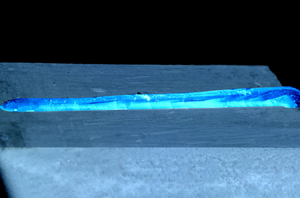
Our study takes place in this context and focuses on the solidification of a thread of water, the so-called rivulet. In a recent experimental study (Monier et al. Reference Monier, Huerre, Josserand and Séon2020), we have shown that when a water rivulet flows on a cold substrate, an ice wall grows and eventually a steady regime is reached where a thin thread of water flows on an ice structure whose thickness is almost linearly growing downstream (see figure 1). In this previous paper, we reported mainly two features. Firstly, a one-dimensional diffusive regime for the initial solidification dynamics was identified. Secondly, the linear ice profile observed in the steady regime was recovered using scaling arguments and considering the confinement of the thermal boundary layer in the water by the free surface.

Figure 1. Frozen rivulet. (a) Experimental picture of the freezing rivulet in the steady state. The water is dyed with fluorescein and appears green under ultraviolet light. The flow goes from left to right. (b) Picture of the remaining frozen structure after the flow was stopped and the remaining water cleaned. Scale bars: 1 cm.
In the present paper we realise a detailed study of this problem, with the derivation and solution of a complete theoretical model considering a half-Poiseuille velocity profile in the water. The quasi-analytical predictions of both the geometrical and the thermal quantities compare well with the experimental results for a whole range of experimental parameters.
Firstly, the experimental set-up and methods are described. Then, the theoretical analysis with the main physical assumptions, the temperature field equations and the main steps for the resolution are presented. Finally, the last section provides a complete physical analysis of the freezing rivulet.
2. Experimental set-up
The experiment consists of flowing distilled water dyed with fluorescein at 0.5 g L $^{-1}$ along a cold aluminium block of 10 cm long, with an inclination of $\alpha =30^{\circ }$ or $\alpha =60^{\circ }$ to the horizontal (see figure 1a). The temperature of the injected water $T_{in}$ ranges from 5 to 49 $^{\circ }$C. The water is injected through a needle (inner diameter 1.6 mm) at a flow rate $Q=20$ mL min $^{-1}$, such that there is no meander at room temperature (Le Grand-Piteira, Daerr & Limat Reference Le Grand-Piteira, Daerr and Limat2006). A straight water rivulet is then formed (Towell & Rothfeld Reference Towell and Rothfeld1966) with a typical width of 2 mm, a thickness of $h_{w}=800$ $\mathrm {\mu }$m and a characteristic velocity of the buoyant flow $U_0\approx 10$ cm s $^{-1}$.
The temperature of the aluminium substrate  $T_{s}$ is set by plunging the block into liquid nitrogen for a given amount of time so that it ranges from $-9$ to $-44\,^{\circ }$C. During the experiment $T_{s}$ is measured and remains constant ( ${\pm }1\,^{\circ }$C). Experiments performed with substrate temperatures below $-44\,^{\circ }$C consistently lead to the fracture (Ghabache et al. Reference Ghabache, Josserand and Séon2016) or the self-peeling of the ice (de Ruiter, Soto & Varanasi Reference de Ruiter, Soto and Varanasi2018) and are not considered here. Upon contact with the cold substrate, the water freezes and an ice layer grows while the water continues to flow on top (see supplementary movie 1 available at https://doi.org/10.1017/jfm.2021.41). During the solidification process, the water retracts on its own ice while flowing to reach a constant width, surprisingly independent of the angle $\alpha$. A direct implication of this observation is that the water thread thickness $h_{w}$ is also independent of the slope $\alpha$.
During the solidification process, the fluorescein concentrates between the ice dendrites, causing self-quenching and fluorescence dimming in the ice (Marcellini et al. Reference Marcellini, Noirjean, Dedovets, Maria and Deville2016). This allows us to clearly distinguish between the ice and the water layers under ultraviolet light. The set-up is placed in a humidity-controlled box to avoid frost formation ( $H_{r} \approx 5\text {--}10\,\%$).
The ice layer thickness  $h_{i}(x,t)$ is then measured using a Nikon D800 camera recording from the side at 30 frames per second. Temperature fields of the water and the ice are measured using an Flir A655sc infrared camera and by setting the average emissivity of ice and water to $\bar {\epsilon } = 0.965$. As the linear attenuation coefficient of water is $J_{b} = 10^6$ m $^{-1}$, the skin depth for the temperature measurement is around 1 $\mathrm {\mu }$m. Videos of the surface temperatures (see supplementary movie 2) of the flowing water were recorded using a $25^{\circ }$ field of view, 25 mm lens ( $\text {1 pixel} = 150$ $\mathrm {\mu }$m) while a close-up lens is added when measuring the transverse temperatures ( $\text {1 pixel}= 50$ $\mathrm {\mu }$m, see supplementary movie 3). Image processing for both the Nikon D800 camera and the infrared camera is based on thresholding methods. For the ice thickness, the threshold is realised from the grey shade values. For the temperature maps, the ice–water interface is detected as follows: when temperature is below 0 $^{\circ }$C, we measure temperatures in the ice, when it is above 0 $^{\circ }$C, we measure temperatures in the water. Discontinuities in the temperature gradients set the positions of the metal–ice and the water–air interfaces.
3. Theoretical analysis
3.1. General assumptions
As the time for solidification (order of minutes) is much larger than the characteristic time of the flow (few seconds for the water to flow down the rivulet), we consider the water flow over a substrate whose quasi-static evolution can be analysed independently. Consequently, both the temperature and the flow depend on time only through the variation of the ice layer thickness. Moreover, the slope of the ice structure remaining small (few degrees), the liquid flow in the quasi-static regime is described using the lubrication approximation. The small value of the Reynolds number ( $Re=U_0h_{w}/\nu \sim 80$) also ensures (with the small ice slope) that the flow is laminar and parallel. We may expect these approximations to fail both at very short times (where the ice layer grows rapidly) and close to the input where the ice slope can be significant. The solution of the problem proposed below should thus be taken with care in these regions (small times and distances from the needle). More precisely, we can estimate the time scale for the velocity profile to establish as $h_w^2/\nu \sim 0.5$ s, which is much smaller than the typical solidification dynamics, and the corresponding length scaling $U_0 h_w^2/\nu \sim 5$ cm, which is a fraction of the total rivulet length (approximately half of it).
Firstly, the water flow is considered parallel to the local ice slope (see figure 2) and the velocity field is  $u$. The quasi-static approximation consists in neglecting the explicit time variation of the velocity. Consequently, as the volumetric flux is set and the solidification rate is slow, the mass conservation implies that the liquid layer thickness $h_{w}$ is constant along the flow direction (Towell & Rothfeld Reference Towell and Rothfeld1966). Within this framework, where the ice thickness does not change with time, the flow is laminar and follows a semi-Poiseuille velocity profile that can be written in the form
 \begin{equation} u(x,z)= U_0 \frac{z-h_{i}(x)}{h_{w} }\left( 2 - \frac{z-h_{i}(x)}{h_{w}} \right), \end{equation}
where  $U_0$ is the free surface velocity. For this two-dimensional (2-D) geometry, $U_0$ is obtained by a balance between the downslope gravity and the viscous forces, yielding $U_0=({g h_{w}^2}/{2 \nu }) [\sin (\alpha )-h_{i}'(x)\cos (\alpha )] \sim ({g h_{w}^2}/{2 \nu }) \sin (\alpha )$, although in our three-dimensional (3-D) geometry, it is a function of the lateral position in the rivulet (Le Grand-Piteira et al. Reference Le Grand-Piteira, Daerr and Limat2006). Finally, let us note that even if the velocity field is along the local slope of the ice layer, we can to good approximation consider that this velocity field holds also along the $x$-direction of the substrate (assuming $|h'_{i}(x,t)| \ll 1$ the error made is only a few per cent).

Figure 2. Notations used in the problem. (a) Lateral view of the water thread (dark blue) flowing on the ice structure (light blue). (b) Close-up schematics with the definition of the three domains on the  $z$-axis, of the temperature fields and of the velocity fields. (c) Schematics of the different temperature fields in the solid, in the ice and in the water.
3.2. Model equations
For the temperature field, we use the static heat equation, incorporating an advection term for the liquid domain. We further assume that the temperature of the ice–substrate interface is a time-invariant natural temperature  $T_{0}$ (de Ruiter et al. Reference de Ruiter, Soto and Varanasi2018), different from the substrate temperature $T_{s}$. This interface temperature corresponds to the solution of the diffusion problem solved when suddenly putting in contact two bodies (substrate and water) at different temperatures. It is deduced from the complete model considering the heat propagation in both the ice and the substrate (Thiévenaz et al. Reference Thiévenaz, Séon and Josserand2019), and is a function of both the melting temperature $T_{m}$ ( $T_{m}=0\,^\circ$C) and the substrate temperature far from the interface $T_{s}$. Following the approach developed in (Thiévenaz et al. Reference Thiévenaz, Séon and Josserand2019) and considering the actual range of experimental parameters, the ice–substrate interface temperature $T_{0}$ is linked to the substrate temperature $T_{s}$ through (3.2),
 \begin{equation} \frac{T_{0}-T_{s}}{T_{m}-T_{s}}=\frac{1}{1+\sqrt{\dfrac{k_{s}\rho_{s}c_{p,s}}{k_{i}\rho_{i}c_{p,i}}}\, \mathrm{Erf}\left(\dfrac{\sqrt{B}}{2}\right)}. \end{equation}
Here,  $B$ is a non-dimensional parameter that is found as a solution for the implicit equation
 \begin{equation} St=\frac{\sqrt{\pi B}}{2} \,\mathrm{e}^{B /4} \left(\sqrt{\frac{k_{i}\rho_{i}c_{p,i}}{k_{s}\rho_{s}c_{p,s}}}+\mathrm{Erf} \left(\frac{\sqrt{B}}{2}\right)\right), \end{equation}
where the Stefan number  $St$ is defined in (3.18), and $k_{(i,s)}$, $\rho _{(i,s)}$ and $c_{p,(i,s)}$ are the thermal conductivities, densities and specific heat capacities of the ice and the substrate, respectively. We checked experimentally the time evolution of the ice temperature at the substrate contact point and we measured $T_0$ constant and equal to its theoretical value. The model is written for a 2-D geometry ( $x$ and $z$ in figure 2) although the thickness of the rivulet is approximately half of its width. However, we expect the results of the model to give pertinent predictions for the rivulet, in particular close to its centreline.
We thus use the following set of equations for the temperature fields (see a schematic presentation of the model on figure 3).

Figure 3. Summary of the model hypotheses: a layer of ice lies between the water ( $h_{i}+h_{w}>z > h_{i}$) and the semi-infinite substrate ( $z < 0$). The temperature of the substrate–ice interface is set constant at $T = T_{0}$ and that of the ice–water interface is set constant at the melting point ( $T = T_{m}$). The temperature in the ice and the water is given by a set of two heat equations, coupled at $z = h_{i}$ by the temperature continuity and by the Stefan condition (imposing the difference of thermal fluxes to be equal to the latent heat liberated by the freezing). The velocity field in the water $u(z)$ is taken as a semi-Poiseuille with $U_0$ the velocity at the free surface $z=h_{i}+h_{w}$.
In the ice,  $0\leq z \leq h_{i}(x,t)$, the temperature field $T_{i}(x,z)$ follows
 \begin{equation} \frac{\partial^2 T_{i}}{\partial z^2} + \frac{\partial^2 T_{i}}{\partial x^2}=0 \end{equation}
and in the water,  $h_{i}(x,t)\leq z \leq h_{i}(x,t)+h_{w}$, the temperature field $T_{w}(x,z)$ follows the quasi-static advection–diffusion equation
 \begin{equation} u \frac{\partial T_{w}}{\partial x} = D_{w} \left( \frac{\partial^2 T_{w}}{\partial z^2} + \frac{\partial^2 T_{w}}{\partial x^2} \right). \end{equation}
 In the latter equation, the advection term can be taken in the  $x$-direction only. Indeed, the fluid flux (20 g min $^{-1}$) is large compared with the volumetric rate of growth of the ice (few mg min $^{-1}$), and consequently the flow can be considered parallel. Moreover, in this framework, both the advection time ( $\sim$1 s) and the diffusion time ( $\sim$10 s) are much smaller than the typical growth time of the frozen rivulet (few minutes), justifying the use of the quasi-steady equations. Taking $Z=h_{w}$ as the typical vertical length scale for the temperature variation, the horizontal length scale $X$ scales as
 \begin{equation} \frac{U_0}{X} \sim \frac{D_{w}}{h_{w}^2},\quad \textrm{leading to}\ X \sim Pe \,h_{w}, \end{equation}
where the Péclet number is defined by  $Pe=U_0h_{w}/D_{w}$. From the experiments, we have the following values: $D_{w} = 1.4 \times 10^{-7}$ m $^2$ s $^{-1}$; $h_{w} \sim 800$ $\mathrm {\mu }$m; $U_0 \sim 0.1$ m s $^{-1}$. This suggests that $Pe \sim 600$, demonstrating that the horizontal length scale is much larger than the vertical one so that the horizontal derivatives can be neglected in the right-hand side of (3.5) compared with the vertical derivatives (namely $|\partial _{xx}| \ll |\partial _{zz}|$ in the Laplacian term).
The following boundary conditions have to be imposed to the temperature fields. Firstly the substrate temperature  $T_0$ at the interface with the ice $z=0$. Then, we impose the melting temperature at the ice–water interface $z=h_{i}(x,t)$. This condition corresponds to the continuity of the temperature at the ice–water interface, $T_{m}$ that we take constant, neglecting its dependence on the interface curvature or velocity (Gibbs–Thomson and kinematic corrections, respectively, Langer (Reference Langer1980), Worster (Reference Worster2000), De Ruiter et al. (Reference De Ruiter, Colinet, Brunet, Snoeijer and Gelderblom2017) and Herbaut et al. (Reference Herbaut, Brunet, Limat and Royon2019)).
The heat flux balance at the air–water interface,  $z=h_{i}(x,t)+h_{w}$, requires a detailed analysis. Indeed, the heat transfer stems from three different contributions: conduction, evaporation and radiation. Considering the very low thermal conductivity of the air, conduction in the air can be safely neglected. Furthermore, we can estimate the temperature change occurring in water considering radiative effects on the one hand and evaporative cooling on the other hand. Considering the laboratory as a black body at temperature $T_\infty = 300$ K and our frozen rivulet as a black body at temperature $T_{m}$, the temperature increase of the water resulting from the radiative heating is 0.13 $^{\circ }$C, therefore negligible in these experiments. The evaporative flux can be estimated through the use of the Prandlt–Blasius–Pohlhausen boundary layer in which we considered a typical air velocity arising from two sources. The first one is the air flow generated by the rivulet itself, with a typical velocity of $10$ cm s $^{-1}$. The second one is the flow coming from the presence of a heat source (the water) in a cold environment. In our experiments, the maximum air velocity is $3.6$ cm s $^{-1}$ for extreme temperature differences of 90 $^{\circ }$C. The temperature decrease estimated from these evaporative fluxes remain below 1 $^{\circ }$C. Consequently, in our model we disregard all these heat transfer contributions and consider a zero thermal flux condition at the free surface.
In addition, the entry temperature  $T_{in}$ is prescribed at $x=0$ in the water domain, imposing $h_{i} (0,t)=0$. Therefore, the final system of equations to be solved for determining the temperature fields both in the ice and the water domains is exposed below ((3.7) to (3.11)).
In the ice,  $0\leq z \leq h_{i}(x,t)$, the temperature is solution of
 \begin{equation} \frac{\partial^2 T_{i}}{\partial z^2} =0. \end{equation}
 In the water,  $h_{i}(x,t)\leq z \leq h_{i}(x,t)+h_{w}$, it is solution of
 \begin{equation} u \frac{\partial T_{w}}{\partial x} = D_{w} \frac{\partial^2 T_{w}}{\partial z^2}. \end{equation}
The boundary conditions at the interfaces follow
 \begin{equation} T_{i}(x,0)=T_0,\quad T_{i}(x,h_{i})=T_{w}(x,h_{i})=T_{m}\quad \textrm{and} \quad \frac{\partial T_{w}}{\partial z} (x,h_{i}+h_{w})=0. \end{equation}
 The water temperature at injection,  $h_{i}(0,t)\leq z \leq h_{i}(0,t)+h_{w}$ writes as
 \begin{equation} T_{w}(0,z)=T_{in}. \end{equation}
Finally, the evolution of the ice layer thickness is described by the Stefan condition, coupling the thermal fluxes at the ice–water interface through
 \begin{equation} \rho_{i} \mathcal{L} \frac{\partial h_{i}}{\partial t}= k_{i} \frac{\partial T_{i}}{\partial z} (x,h_{i})-k_{w} \frac{\partial T_{w}}{\partial z} (x,h_{i}), \end{equation}
where  $\mathcal {L}$ is the latent heat of solidification and $k_{i,w}$ are the thermal conductivities of the ice and water, respectively, related to their diffusion coefficients through the general relation $k_{(i,w)}=\rho _{(i,w)}c_{p,(i,w)}D_{(i,w)}$. The Stefan condition in (3.11) is written considering the ice slope $\beta$ to be small so that the gradients can be approximated by their $z$-direction component. This equation is the only one containing a time derivative in our approach, a consequence of the larger time scale of ice formation (few minutes) compared with all the other time scales in the problem: establishments of the velocity profile (1 s) and of the thermal boundary layer (5 s). Therefore, all the temperature fields will depend on time through the (slow) time variation of $h_{i}$ only. In fact, the temperature field in the solid is not a priori connected with the temperature field in the liquid film. The coupling between these two domains (liquid film and ice layer) is reduced to the Stefan condition that controls the evolution of $h_{i}(x,t)$. It directly follows from the fact that the boundary condition at the ice–water interface $T=T_{m}$ does not depend on time neither on $h_{i}$ nor other parameters in our system. Consequently, the two thermal problems (water and ice domains) are totally independent and can be solved separately, the time evolution being subjected to the variation of $h_{i}$ through the Stefan equation.
In the fluid domain, the set of equation and boundary conditions is similar to the so-called Graetz problem for laminar flows, written here in its 2-D version (Graetz Reference Graetz1885; Fehrenbach et al. Reference Fehrenbach, de Gournay, Pierre and Plouraboué2012). Indeed, the free surface no-flux boundary condition for the temperature (3.21) plays the role of a symmetry condition for a liquid flowing between two plates located at  $z=0$ and $z=2h_{w}$ while the semi-Poiseuille velocity profile also exhibits this symmetry.
3.3. Dimensionless problem
The system of equations can be made dimensionless using the two typical length scales introduced above,  $h_{w} Pe$ and $h_{w}$ for the horizontal and vertical directions, respectively. Dimensionless temperature fields are introduced for each domain. In the water we define
 \begin{equation} \theta_w=\frac{T_{w}-T_{m}}{T_{in}-T_{m}},\quad \bar{z} = \frac{z-h_{i}(x)}{h_{w}} \quad \textrm{and}\quad \bar{x} = \frac{x}{h_{w}Pe}. \end{equation}
In the ice we use
 \begin{equation} \theta_i=\frac{T_{i}-T_0}{T_{m}-T_0},\quad \bar{z}_i=\frac{z}{h_{w}}, \quad \bar{x}=\frac{x}{h_{w}Pe}\quad \textrm{and} \quad \bar{h}_{i}=\frac{h_{i}}{h_{w}}. \end{equation}
The time is rescaled using the ice thermal diffusion coefficient yielding
 \begin{equation} \bar{t}=D_{i} t/h_{w}^2. \end{equation}
The system of equations to be solved then read as
 \begin{equation} \frac{\partial^2 \theta_i}{\partial \overline{z_i}^2} = 0, \end{equation}
 \begin{equation}\bar{z}(2-\bar{z}) \frac{\partial \theta_w}{\partial \bar{x}} = \frac{\partial^2 \theta_w}{\partial \bar{z}^2} \end{equation}
and
 \begin{equation} \frac{ \partial \bar{h}_{i}}{\partial \bar{t}}(\bar{x},\bar{t})= St \left(\frac{ \partial \theta_i}{\partial \overline{z_i}}(\bar{x},\bar{h}_{i})-\frac{k_{w}}{k_{i}} \frac{1}{\bar{T}} \frac{\partial \theta_w}{\partial \bar{z}}(\bar{x},0) \right), \end{equation}
where the Stefan number,
 \begin{equation} St= \frac{C_{p,i} (T_{m}-T_0)}{\mathcal{L}}, \end{equation}
compares the heat necessary to bring the ice temperature from the substrate temperature to the melting temperature with the latent heat of solidification.
The boundary conditions read as
 \begin{gather} \theta_w(0,\bar{z} ) =1;\quad T_{in} \textrm{ at the entrance}, \end{gather}
 \begin{gather}\theta_w(\bar{x},0) = 0; \quad T_{m} \textrm{ at the water--ice interface}, \end{gather}
 \begin{gather}\frac{\partial \theta_w}{\partial \bar{z}}(\bar{x},1)= 0; \quad \textrm{insulating water--air interface -- no flux}, \end{gather}
 \begin{gather}\theta_i(\bar{x},0) =0;\quad T_0 \textrm{ at the metal--ice interface}, \end{gather}
 \begin{gather}\theta_i(\bar{x},\bar{h}_{i}) = 1;\quad T_{m} \textrm{ at the water--ice interface}. \end{gather}
Finally, the reduced temperature
 \begin{equation} \bar{T}=\frac{T_{m}-T_0}{T_{in}-T_{m}} \end{equation}
plays the role of the control parameter of the problem.
3.4. Model solution
As explained above, the two thermal equations (3.16) and (3.15) can be treated independently, since the variations of  $\bar {h}_{i}(\bar {x},t)$ do not intervene explicitly.
Firstly, the resolution of (3.15) is straightforward in the ice layer,
 \begin{equation} \theta_i= \frac{\bar{z}_i}{\bar{h}_{i}}=\frac{z}{h_{i}(x,t)}. \end{equation}
On the other hand, the temperature field in the water can be deduced from a 2-D Graetz problem and we recall here the main properties of this solution (Incropera et al. Reference Incropera, Lavine, Bergman and DeWitt2007). Using the linearity of (3.16) and separation of variables, we can exhibit a quasi-analytical solution of the problem.
More precisely, we seek solutions of the equation for  $0\le \bar {z} \le 1$ in the form
 \begin{equation} \theta_w(\bar{x},\bar{z})= \sum_{n=1}^{\infty} \theta_n(\bar{x},\bar{z})=\sum_{n=1}^{\infty} A_n \varPhi_n(\bar{z}) \,\textrm{e}^{-\lambda_n^2 \bar{x}}, \end{equation}
where  $\varPhi _n$ and $\lambda _n$ are the eigenfunctions and the eigenvalues, respectively, of the following Sturm–Liouville problem, composed of the equation
 \begin{equation} \varPhi_n''={-}\lambda_n^2 \bar{z} (2-\bar{z}) \varPhi_n \end{equation}
and the boundary conditions
 \begin{equation} \varPhi_n(0)=0\quad \textrm{and} \quad \varPhi_n'(1)=0. \end{equation}
 The eigenfunctions  $\varPhi _n$ involve cylindrical functions and the boundary conditions lead to a discrete infinite set of positive eigenvalues $\lambda _n$. To evaluate the coefficients $A_n$ in (3.26), we apply the last boundary condition (3.19), which specifies the temperature at the inlet. Using the orthogonal property of the Sturm–Liouville system, we obtain
 \begin{equation} A_n=\int^1_0 \varPhi_n(\bar{z}) \bar{z} (2-\bar{z}) \,\textrm{d}\bar{z}. \end{equation}
The coefficients  $A_n$ and $\lambda _n$ as well as the functions $\varPhi _n$ are provided in the Appendix.
Figure 4(a) shows the temperature map of the solution: as  $\bar {x}$ increases, we can observe the growth of the thermal boundary layer starting from $\bar {z}=0$ at $\bar {x}=0$ due to the cooling of the liquid from the plate, as the liquid flows. The size of this boundary layer,
 \begin{equation} \delta(\bar{x})=\frac{1}{\dfrac{\partial \theta_w}{\partial \bar{z}}(\bar{x},0)}, \end{equation}
defined as the inverse of the temperature slope at  $\bar {z}=0$, is indicated on the map as a black solid line. At small horizontal scales, $x\ll 1$, it can be shown that $\delta (\bar {x}) \propto \bar {x}^{1/3}$ (see inset of figure 4a) and we observe that the boundary layer in fact reaches the liquid film thickness for $\bar {x} \sim 0.2$. Further on, we notice that the surface temperature $\theta _w(\bar {x},1)$ decreases rapidly, as illustrated on figure 4(b).

Figure 4. (a) Colour map of the temperature field in the liquid layer, solution of (3.16) with the associated boundary conditions. The solution is shown in dimensionless units, and the colour scale is indicated on the right-hand side. The solid line shows the growth of the thermal boundary layer defined in (3.30). Inset: log–log plot of the thermal boundary layer exhibiting a 1/3 power law. (b) Temperature at the free surface,  $\theta _{surf}(\bar {x})=\theta _w(\bar {x},1)$.
Finally, one can show from (3.26) that the solution of the equation is well approximated by its first mode already for  $\bar {x}>0.05$, leading to
 \begin{equation} \theta_w(\bar{x},\bar{z}) \sim A_1 \varPhi_1(\bar{z})\, \textrm{e}^{-\lambda_1^2 \bar{x}} \end{equation}
and predicting an exponential decrease of the water surface temperature for  $\bar {x} \geq 0.05$, as observed in figure 4(b). For the experiments, it means that this single mode temperature field is valid for $x \geq 0.05 \, h_{w} \, Pe \sim 2$ cm, which is a fraction of the substrate length.
4. Physical analysis
Using our experimental tools and the theoretical model proposed before, we can now proceed to a complete physical analysis of the freezing rivulet. We start by studying the ice layer growth.
4.1. Formation of the ice layer
4.1.1. General description of the rivulet growth
Figure 5(a) presents the ice layer thickness as a function of time for two different positions along the substrate ( $x=2$ and 8 cm), for $T_{in} = 11\,^{\circ }$C and $T_0 = -11.4\,^{\circ }$C ( $\bar {T}=-T_0/T_{in}=1.04$).

Figure 5. Ice structure growth. (a) Ice thickness over time for two different plane positions ( $\alpha = 30 ^{\circ }$, $T_{in} = 11\,^{\circ }$C, $T_0 = -11.4\,^{\circ }$C). The ice growth is first diffusive and then converges exponentially towards a maximum value $h_{max}(x)$. Inset: $(h_{max}(x)-h_{i}(x,t))/h_{max}(x)$ as function of the time in a lin–log scale. Here $\tau$ is defined as the characteristic time scale. (b) Profile of the frozen rivulet at the end of the experiment, for the same parameters. After an entry zone of length $x_{0}$, the ice thickness profile is linear, characterised by its angle $\beta$. In both figures, error bars are smaller than the marker size.
As shown in a previous study (Monier et al. Reference Monier, Huerre, Josserand and Séon2020), at early times the ice layer grows homogeneously along the plane following a diffusive dynamics  $h_{i}(t)=\sqrt {BD_{i}t}$, where $B$ is defined in (3.3). In this regime, the thickness profiles are parallel to the substrate.
After this diffusive regime, we observe a second regime where the ice layer continues to grow until it reaches a maximum height  $h_{max}(x)$ that increases along the plane. The inset of figure 5(a) presents the same data set but using a logarithmic scale for the normalised difference to the final ice height $(h_{max}(x)-h_{i}(x,t))/h_{max}(x)$. It shows that, in this second regime, the ice thickness converges exponentially towards its asymptotic value following $(h_{max}(x)-h_{i}(x,t))/h_{max}(x) \sim A(x)\,\textrm {e}^{-t/\tau }$.
Finally, the ice layer stops growing and the system reaches a permanent regime consisting of a static ice structure, of thickness  $h_{max}(x)$, on top of which a water thread is flowing. Such a permanent regime can be understood qualitatively by considering the thermal fluxes at the ice–water interface where the temperature is always at the melting temperature (0 $^\circ$C). The water is dispensed at a constant temperature, inducing the development of a thermal boundary layer that imposes a temperature gradient perpendicular to the ice–water interface, constant in time. On the other side of the interface, the temperature gradient in the ice can be estimated with $(T_{m}-T_0)/h_{max}(x)$. At early times, the ice layer is very thin and the gradient is high. Consequently, the ice grows in order to decrease its temperature gradient and stops when the heat fluxes on both sides of the ice–water interface balance. Figure 5(b) presents the maximum height reached by the ice layer, $h_{max}(x)$, as a function of $x$. After a first entry zone, characterised by a steep ice thickness increase, $h_{max}(x)$ is well described by a line of slope $\beta$ as illustrated by the dashed line: $h_{max}(x)=h_{i,0}+\beta (x-x_0)$. In the following, we will show that this linear height profile is due to the heat balance between the ice layer and the liquid rivulet, and is deeply related to the fact that the thermal boundary layer has reached the rivulet thickness $h_{w}$.
4.1.2. Theoretical permanent ice thickness profile
Knowing the temperature field in both domains (water and ice), we can write the evolution equation for the ice layer thickness. This equation is valid within the quasi-static approximation made here, where the time variations of the fields are simply subjected to the evolution of  $\bar {h}_i(\bar {x},\bar {t})$. In this context, the Stefan equation (3.17) leads to the equation for $\bar {h}_i(\bar {x},t)$,
 \begin{equation} \frac{\partial \bar{h}_i}{\partial \bar{t}}(\bar{x},\bar{t})= St \left(\frac{ 1 }{\bar{h}_i}-\frac{k_{w}}{k_{i}} \frac{1}{\bar{T} }\frac{\partial \theta_w}{\partial \bar{z}}(\bar{x},0) \right), \end{equation}
where we have used the constant gradient solution from (3.25) for the temperature in the ice layer. Then  $\theta _w$ is taken as the general solution for the water temperature field, that we might approximate by its first mode for $\bar {x}>0.05$, given by (3.31). We can thus deduce the final shape of the ice layer, valid in our experiment for $x>2.5$ cm,
 \begin{equation} h_{max}(x) = h_{w} \bar{T} \frac{k_{i} }{k_{w}} \frac{1}{A_1} \frac{1}{\varPhi_1' (0)} \exp\left( \lambda_1 ^2 \frac{x-x_0}{h_{w} Pe}\right). \end{equation}
In the next two sections, we study how the rivulet reaches this permanent regime and how this theoretical prediction compares with the experimental measurements.
4.1.3. Convergence to the static shape
Following the initial diffusive growth, we wonder how the ice dynamics reaches its static shape. We develop an asymptotic analysis around the stationary state,  $h_{i}(x,t)=h_{max}(x) (1+\epsilon f(t))$, with $\epsilon \ll 1$. Substituting in (4.1) gives a differential equation for $f$,
$f$,
 \begin{equation} f'(t)=\frac{-St\,D_{i}}{h_{max}^2}f(t). \end{equation}
It confirms the exponential behaviour of the ice growth towards its static shape that we observed experimentally (see figure 5a). Subsequently, we can determine the characteristic time  $\tau$ using the theoretical prediction of the final ice shape given by (4.2),
 \begin{equation} \tau=\frac{h_{max}^2}{D_{i}\,St} = \frac{h_{w}^2}{D_{i}}\frac{\bar{T}^2 }{St} \left(\frac{k_{i} }{k_{w}} \frac{1}{A_1} \frac{1}{\varPhi_1' (0)}\right)^2 \exp \left(2\lambda_1 ^2 \frac{x-x_0}{h_{w} Pe}\right). \end{equation}
 Figure 6 presents the convergence time obtained from the measure of  $h_{max}$ as a function of its theoretical prediction (right-hand side of (4.4)). A direct measurement of $\tau$ from the fit of the data in the inset of figure 5(a) was too noisy to be used. For the different physical parameters, we use $k_{i}=2.1$ and $k_{w}=0.58$ W m $^{-1}$ K $^{-1}$, $h_{w}=800$ $\mathrm {\mu }$m, $D_{i} = 1.2\times 10^{-6}$ m $^{2}$ s $^{-1}$, $c_{p,i} = 2090$ J kg $^{-1}$ K $^{-1}$, $\mathcal {L} = 3.3 \times 10^{5}$ J kg $^{-1}$ and $Pe=570$. Here $\lambda _1$, $A_1$ and $\varPhi _1'(0)$ are numerically evaluated as $1.68$, $0.78$ and $2.2$, respectively. This comparison is particularly convincing, since the coefficient between the two times is always around 0.7, very close to 1. It provides a first validation of the theoretical prediction of the static ice shape $h_{max}$ and consequently of the entire model that led to this prediction. Moreover, it allows us to forecast the characteristic time it takes for the rivulet to reach its maximum height. Finally, it predicts that this time scales as $\bar {T}^2 /St \propto (T_{m}-T_{0})/(T_{in}-T_{m})^2$ indicating that the variation of water temperature is the main parameter to control the convergence time.

Figure 6. Experimental convergence time  $h_{max}^2/(D_{i}\,St)$ against theoretical convergence time as predicted by (4.4), for a plane inclination of $\alpha = 30^{\circ }$. Markers stand for the positions along the plane and the colour code is for $\bar {T}^2/St$.
Although the agreement between the model and the experiments is very good with regards to the approximations made, we observe some discrepancies (the fit of the data gives a slope  $0.7$ instead of $1$ in figure 6, the results are spread) that can be attributed to different factors. Firstly, we have taken a constant $h_{w}$ over the experiments while it varies slightly with the temperatures, witnessing probably a variation of the wetting properties of the water on ice. Moreover, since the experiments were performed with non-degassed water, we always observe bubbles in the part of the ice close to the substrate (see for example the difference of colour in the ice on figure 1(a)). The effect of bubbles in the ice during experiments of freezing of capillary objects is currently being investigated (Chu et al. Reference Chu, Zhang, Li, Jin, Zhang, Wu and Wen2019) and composite models can be used to predict the conductivity when knowing the concentration, organisation and size of the bubbles in the ice (Wegst et al. Reference Wegst, Schecter, Donius and Hunger2010). Typically, a reduction of a factor two in the conductivity would correspond to 20 %–30 % of air in the ice, consistent with the typical front velocity at the beginning of our experiment $\sim$5 mm min $^{-1}$ (Carte Reference Carte1961). We thus believe that an effective thermal conductivity $k_{i}$ (or even varying with space) should be considered in the ice to account more finely for the experimental observations.
4.1.4. Experimental permanent ice thickness profile
After the two regimes of growth fully characterised before – a diffusive one followed by an exponential relaxation – the ice reaches a static shape. Figure 1 shows two examples of such a shape, and figure 5(b) is a plot of a typical permanent ice thickness profile. As we saw, the experimental profile is linear and can be written as  $h_{max}(x) = h_{i,0} + \beta (x-x_0)$. Theoretically, this thickness profile is given by (4.2), where the experimental values of $x$ (
$x$ ( $\bar {x}>0.05$, that is $x>2.5$ cm) allow us to consider only the first mode and to expand the exponential term. We thus recover the linear relationship between $h_{max}$ and $x$,
$x$,
 \begin{align} h_{max}(x) & \sim h_{w} \bar{T} \frac{k_{i} }{k_{w}} \frac{1}{A_1} \frac{1}{\varPhi_1' (0)} \left(1+ \lambda_1 ^2 \frac{x-x_0}{h_{w} Pe}\right) \end{align}
 \begin{align} & = 1.7 \times 10^{{-}3} \bar{T}+ 1.1 \times 10^{{-}2}\bar{T}(x-x_0). \end{align}
 Figure 7(a) shows the thickness of the ice at the beginning of the linear profile  $h_{i,0}$ obtained on the experimental profiles, as a function of the reduced temperature $\bar {T}$. The data clearly exhibit a linear trend and a fit, represented as a dashed line on figure 7(a), gives a coefficient $1.8\times 10^{-3}$ m. This value, very close to the prediction of $1.7\times 10^{-3}$ m, highlights the very good performance of the model. In figure 7(b), the experimental values of the slope $\beta$ are plotted as a function of $\bar {T}$. Again, the linear behaviour is recovered and the dotted line around which all the data gather is $\beta =1.7\times 10^{-2}\,\bar {T}$, of the same order as the theoretical one. Overall, these two plots show that the model is well suited to predict the maximum ice thickness profile, even though we had to expand the exponential term.

Figure 7. Permanent ice structure profile. (a) Measured  $h_{i,0}$ against $\bar {T}$, the dashed line is the best fit of the data: $1.8\times 10^{-3}\,\bar {T}$. Colours stand for the substrate–ice interface temperature $T_{0}$ and markers for the plane inclination. Error bars are smaller that marker size. (b) Measured slope $\beta$ of the ice profile against $\bar {T}$. Colours stand for the substrate–ice interface temperature and markers for the plane inclination.
It is interesting to note that, for a much longer plate, as soon as the rivulet departs from the linear regime, most of the assumptions made will break down: the slope of the ice layer will become large and the gravity might rapidly lose its role, changing drastically the flow. Consequently, the exponential profile will most probably never be reached but as the flow will rapidly become completely different, the ice structure might exhibit a succession of humps and hollow or some other unexpected shapes.
4.2. Temperature fields
4.2.1. Transverse temperature profiles
We were able for a few experiments to measure the temperature maps of the rivulet while flowing, in a small region of the plane. This region is situated between  $x= 2$ and $x=5$ cm, that is roughly at the end of the thermal boundary layer regime and at the beginning of the free surface regime (where the thermal boundary layer thickness is of the order of the rivulet height $h_{w}$). The infrared camera resolution of 50 $\mathrm {\mu }$m allows us to record around 20 measurement points along $z$ in the water and between 20 and 60 in the ice. Keeping in mind that the camera records the temperature at the lateral surface of the rivulet, we compare in the following the experimental results with the theoretical expressions of the temperatures in the ice and in the water obtained in § 3.4.
The temperature field shown in figure 8(a) is obtained with the infrared camera placed on the side of the rivulet in the permanent regime. The temperature is colour-coded according to the colour bar in the left-hand corner of figure 8(a). The line  $T=T_{m}=0\,^\circ$C is represented in white and corresponds to the ice–water interface. The water, appearing in red, is flowing from left to right, on the ice, appearing in blue. The ice structure has reached its static shape, it is not growing anymore. We thus recognise the angle $\beta$ formed by the ice structure. A measurement on this picture gives $\beta =1.7^\circ$, consistent with the prediction from figure 7(b), considering that $\bar {T}=1.85$ in this experiment. We observe on this map the transverse temperature gradient across the whole structure: the temperature increases from $T_{0}=-37\,^\circ$C at the ice–substrate interface to $T=T_{m}=0\,^\circ$C at the ice–water interface, and up to the water–air surface temperature, that is close to $24\,^\circ$C, the injection temperature of the water $T_{in}$. The water–air surface temperature will be discussed later.

Figure 8. Cross-section temperature profiles and model. (a) Experimental picture of the temperature fields in the water (red) and in the ice (blue). Here  $z=0$ corresponds to the substrate–ice interface. (b) Experimental and theoretical profiles ((3.25) and (3.26)). To plot the theoretical temperature profiles, the velocity $U_0$ was adjusted to 19 cm s $^{-1}$ (consistently with experimental estimates), the inlet temperature was set to $T_{in}=20\,^\circ$C, the water thickness $h_{w}=0.9$ mm to its measured value and the origin of the $x$-axis was shifted by 3.8 cm.
To go further in the quantitative analysis, temperature profiles can be extracted from this temperature field. The three graphs on figure 8(b) show the temperature profiles, corresponding to the temperature map above, at three different positions on the plane:  $x=2$, 3.5 and 5 cm. The experimental points are colour-coded in the same way as in the map. The origin of the $z$-axis is taken on the metallic plane. As a consequence, the ice–water interface, localised by the discontinuous temperature gradient, is at a different height in each graph.
The experimental temperature profile in the ice is mainly linear except in a thin zone close to the substrate ( $z\leqslant 0.5$ mm). This deviation from the linear profile is a signature of the temperature field in the substrate (Thiévenaz et al. Reference Thiévenaz, Séon and Josserand2019). Consequently, the linear model given by (3.25) and plotted with a dashed line is very satisfying close to the ice–water interface and becomes more approximate near the substrate. Note that the substrate temperature measured with a thermocouple directly on the metal is $T_{s}=-44\,^\circ$C and the temperature of the ice in contact with the substrate is $T_{0}=-37\,^\circ$C. This difference is perfectly consistent with the relation between $T_{0}$ and $T_{s}$ given by (3.2) that we deduced from a complete model considering the heat propagation in both the ice and the substrate.
In the water, the experimental temperature profiles, appearing in red, highlight the thermal boundary layer behaviour: the temperature is almost constant in a zone close to the free surface. We also notice on the profiles that this zone reduces in size as we go downstream. The theoretical temperature profiles given by (3.26) are plotted with dashed lines on the same graphs. They superimpose perfectly onto the experimental profiles in the three cases. Therefore, the model precisely reproduces the flux at the ice–water interface, the surface temperature and the variation in the water bulk.
Finally, we clearly observe a discontinuity in the temperature slopes at the ice–water interface, testifying the difference in conductivities of the two media (3.11). A measurement of the experimental temperature slopes, with a linear fit on the nine first points in each phase, gives  $k_{i}/k_{w}=2.34$. This ratio should be equal to 3.6 by taking the conductivity values for pure ice and water. As we discussed before, we attribute the difference between our experimental measurement of $k_{i}/k_{w}$ and the one given by the pure body values to the variation of thermal conductivity in ice due to the inclusion of bubbles. Consequently, by taking the conductivity of pure water, this experimental measurement can give us an estimation of the thermal conductivity of our ice in the presence of bubbles, we find $k_{i}=1.36$ W m $^{-1}$ K $^{-1}$. Interestingly, this effect could explain the discrepancy observed in figure 6 for the experiments that last long (blue points). For these long experiments, we consistently observed a very thick ice layer with a big zone full of bubbles and one free of bubbles. We can thus expect the thermal conductivity in these experiments to be smaller and the theoretical convergence time to be reduced consistently.
4.2.2. Comparison of the convective to conductive heat transfer
This section aims at comparing the heat transfer by convection from the ice–water interface to the moving liquid and by pure conduction (diffusion) to a hypothetically motionless liquid. This demands the computation of the Nusselt number of our experiment. It is here defined as the ratio of the conductive to the convective thermal resistance of the fluid (Incropera et al. Reference Incropera, Lavine, Bergman and DeWitt2007),
 \begin{equation} Nu= 4\frac{\displaystyle\frac{\partial T_{w}}{\partial z}(z=h_{i})}{\displaystyle\frac{\left\langle T \right\rangle-T_{m}}{h_{w}}}. \end{equation}
We define the mean temperature  $\left\langle T \right\rangle$ by expressing the rate at which thermal energy is advected with the fluid ( $\rho \left\langle u \right\rangle h_{w}c_{p} \left\langle T \right\rangle$) with integration over the cross-section
 \begin{equation} \left\langle T \right\rangle =\frac{\displaystyle\int_{0}^{h_{w}}u T\, \textrm{d}z}{h_{w} \left\langle u \right\rangle}, \end{equation}
where  $\left\langle u \right\rangle = 2U_0/3$ is the flow mean velocity. This amounts to considering the average temperature weighted by the fluid velocity. To do so, the numerical integration of the advected experimental temperature profile is performed assuming the theoretical half-Poiseuille velocity field used in the previous analysis. Moreover, as discussed in the previous section, the conductive thermal flux at the ice–water interface ( $\partial T_{w}/\partial z (z=h_{i})$), can be deduced from the experimental temperature profiles, for different positions along the plane.
Figure 9 presents with a dashed line (thick) the theoretical prediction of the Nusselt number  $Nu$ derived from the model presented above. As expected from the symmetry of our model, the $Nu$ dashed curved line converges toward a value of 7.54, which compares well to the value obtained for a fully developed laminar flow in a Hele-Shaw cell (Incropera et al. Reference Incropera, Lavine, Bergman and DeWitt2007). In this estimation the velocity profile appearing in $\langle T\rangle$ is not measured, and we used the half-Poiseuille field of the theoretical analysis. The experimental values of the Nusselt number do not correspond perfectly to this 2-D prediction, although the tendency and the order of magnitude are correct. In fact, we can adapt our 2-D model to obtain predictions for a 3-D rectangular duct, where the rivulet width would be denoted $a$ and its thickness ( $h_{w}$ for us) denoted $b$, as shown in the schematic diagram on the top right corner of figure 9. Our 2-D model corresponds thus to the null aspect ratio ( $b/a=0$). The horizontal dashed lines (thin) represent the known asymptotic values found for such ducts with an aspect ratio of $b/a=20$ and $10$, from top to bottom, respectively (Shah & London Reference Shah and London2014). Even though we do not clearly reach any asymptotic regime for $Nu$ in our experiment, we can forecast a plateau value for $Nu$ between 6 and 7. This value is close to the case of a duct with an aspect ratio between 10 and 20. It shows that in our experiment, we have a small effect of the 3-D geometry of the rivulet, reducing slightly the efficiency of the heat transfer as compared with the ideal 2-D model.

Figure 9. Nusselt number as a function of the normalised positions on the plane. Experimental data points,  $\circ$ (red); theoretical curve derived from the theoretical water temperature field,
 ![]() ; asymptotic value of
; asymptotic value of  $Nu$ found for a rectangular duct of aspect ratio 1/20,
 ![]() ; asymptotic value of
; asymptotic value of  $Nu$ found for a rectangular duct of aspect ratio 1/10,
 ![]() .
.
4.2.3. Surface temperature
Figure 10(a) shows a typical experimental temperature field measured from above. The water is injected on the left and flows downward, to the right. The image is taken in the permanent regime. As indicated on the colour bar on the left of this temperature field, the positive temperatures (water) are colour-coded in red whereas the negatives ones (ice) are colour-coded in blue. It is first interesting to notice that we observe a layer of ice wider than the water layer. A possible explanation for this effect is the difference of wetting properties of water on metal and on ice (Thiévenaz et al. Reference Thiévenaz, Josserand and Séon2020). Before freezing, the water rivulet has a given width on the metal (Towell & Rothfeld Reference Towell and Rothfeld1966), then it freezes and an ice structure grows on the metal. The initial ice layer appears in blue on the temperature field and its width corresponds to the width of the initial rivulet. During the solidification process, the water retracts while flowing to reach a constant width, as shown in red on the picture. The width of a rivulet being a balance between the flow rate, the surface tension and the contact angle, it suggests that there is an evolution of the contact angle during the experiment (Thiévenaz et al. Reference Thiévenaz, Josserand and Séon2020). We also notice in the picture a small entrance zone where the width varies along the flow. This is a direct signature of the injection process with the needle. In the following, the measurements are taken out of this area, in the zone between 2 and 9 cm, materialised by the rectangle in the picture. Remarkably, the length of this transient region is similar to the characteristic growth scale of the viscous and thermal boundary layers, so that we expect our theoretical analysis to be pertinent only outside of this domain.

Figure 10. Surface temperature of the flowing water. (a) Thermal picture of an experiment with  $T_{in} = 35\,^{\circ }$C, and $T_{s} = -19\,^{\circ }$C. The colour bar corresponds to the temperatures in the ice and in the water. (b) Surface temperature measured inside the black square following the black line at the centre. (c) Temperature gradients of all the conducted experiments against $T_{in}$. Markers stand for the angle inclination and the ice–substrate interface temperature $T_{0}$ is colour-coded. The dashed line represents the best fit of the data. (d) Rescaled surface temperature fields $\theta _{surf}$ for two different injection temperatures and inclinations as a function of the rescaled plane position. Here $T_{in}$ is taken as the maximum value measured by the camera close to the needle. The dashed line is the theoretical prediction $\theta _{surf}(\bar {x})=\theta _w(\bar {x},1)$.
Thus, equation (3.31) can be used at the surface ( $\bar {z}=1$, that is $z=h_{w}$) to obtain an approximation for the surface temperature far from the needle,
 \begin{equation} T_{surf}(x)=T_{m}+(T_{in}-T_{m})A_1 \varPhi_1(1) \exp\left(-\lambda_1^2\frac{x}{h_{w}\,Pe}\right). \end{equation}
After linearisation, we obtain a linear variation of the surface temperature along the plane ( $x$-axis) and we deduce a theoretical expression for its slope,
 \begin{equation} \frac{\textrm{d}T_{surf}}{\textrm{d} x}={-}(T_{in}-T_{m})A_1 \varPhi_1(1)\frac{\lambda_1^2}{h_{w}\,Pe}. \end{equation}
Interestingly, the model predicts that the slope is linear with the injection temperature of water  $T_{in}$ and does not depend on the ice–substrate interface temperature $T_{0}$.
In order to compare this prediction to our measurements, we extract experimentally the surface temperature. We define it as the maximum value for each  $x$-position on the plane, and it gives the black line drawn in the picture. The corresponding profile is plotted in figure 10(b) and shows the linear decrease of the surface temperature along the plane predicted by the model. This linear decrease is retrieved for all experiments. Figure 10(c) presents the slope of these surface temperature profiles as a function of the inlet water temperature $T_{in}-T_{m}$ for various ice–substrate interface temperatures $T_0$ and two different angles $\alpha$. We observe that the slope is naturally stronger for a higher injection temperature of water and we recover the linear trend with $T_{in}$ predicted by (4.10). The dashed line is a linear fit of the data with a prefactor $-3.2$ m $^{-1}$ that is compatible with the prediction ( $-7.4$ m $^{-1}$). We attribute this discrepancy mainly to the arbitrary choice of the velocity $U_0$ that is present in the definition of the Péclet number and which has been determined within our 2-D model. Furthermore, we also show with this plot that the decrease of the surface temperature of water is independent of the temperature of the substrate–ice interface $T_0$, as was predicted by (4.10). This emphasises the view exposed in the theoretical part: the temperature fields in both the ice and the water are disconnected, leaving the ice thickness as the only parameter ensuring the heat flux continuity.
Finally, figure 10(d) shows four normalised experimental temperature surface profiles  $\theta _{surf}$ obtained for two different angles $\alpha$ and two different injection temperatures $T_{in}$, plotted as a function of $x$ normalised by $h_{w}Pe$. We recover the linear variation observed in 10(b). On the same plot, the black dashed line is the full prediction of the model for the rescaled surface temperature $\theta _w(\bar {x},1)$ as already plotted as a solid line in figure 4. Once again, there is a very good agreement between the theoretical prediction and the experimental results, confirming the suitability of the model to characterise the heat exchange in the frozen rivulet.
5. Conclusion
In this paper we have analysed experimentally and theoretically the formation, growth, final steady shape and temperature fields of a freezing rivulet resulting from a water thread flowing down a cold solid plate. We performed experiments varying the inclination of the plate, its temperature and the water injection temperature.
The model developed is based on the resolution of the heat equations in the ice (diffusion) and in the water (advection–diffusion). In the ice, we found a temperature field varying linearly from the substrate–ice interface temperature to the ice–water interface temperature. In the water, however, the solution is the superposition of different cylindrical functions which is well approximated by its first term to describe the temperature field far from the injection needle.
Interestingly, due to the injection condition (constant temperature), a thermal boundary layer develops, responsible for a temperature gradient in the water and thus a thermal flux at the ice–water interface. This thermal boundary layer thickens with the distance from the needle and reaches the free surface of the rivulet, a few centimetres downstream. Once the boundary layer has established, the heat flux in the water is in fact constant over time. The Stefan boundary condition then governs the ice layer growth rate as long as the thermal fluxes from both sides of the ice–water interface are not equal. This is what we observed experimentally with the existence of three different regimes over time.
In the first one, the ice layer growth is homogeneous along the plane and evolves with the square root of time. This regime is described in a previous paper (Monier et al. Reference Monier, Huerre, Josserand and Séon2020) and well explained by considering the Stefan boundary condition, neglecting the thermal flux in the water. However, increasing the ice layer thickness reduces the thermal flux in the ice and leads inevitably to a second regime where both heat fluxes have to be considered.
We found experimentally that, in this regime, the ice layer thickness converges towards a maximum with an exponential relaxation rate over time. The water temperature is found to be the dominant parameter controlling this convergence time, in good agreement with the model prediction. Finally, when the heat flux in the ice becomes equal to the one in the water, a permanent regime is reached.
There, the ice layer adopts a striking structure, showing a linear thickening with the plane position, located after a small transient region close to the needle where the ice layer is more abrupt. This ice shape is well captured by our model. In order to fully characterise this permanent regime, we used an infrared camera to record the vertical temperature fields in the ice and in the water. The good agreement between these measurements and the developed model highlights the link between the temperature field in the water and the ice layer shape. In a first zone, close to the injection needle, where the thermal boundary layer thickens, the ice layer profile shows a steep increase. After few centimetres, the thermal boundary layer reaches the water–air interface and the water surface temperature starts to decrease along the plane. Measurements of the surface temperature confirm a linear temperature decrease and the model highlights the clear link between this linear decrease and the linear shape of the ice layer. This link is further confirmed by the very good agreement between the model predictions for the geometrical features and the experimental data.
It is important to emphasise that in our approach no adjustable parameter nor macroscopic heat exchange coefficient were needed to account theoretically for the experimental results. Overall, by quantitatively comparing the experiments and the model, our work demonstrates that the dynamics and the final state of a freezing rivulet can be totally determined by the precise balance between the quasi-static thermal fluxes in both domains, water and ice.
Supplementary movies
Supplementary movies are available at http://dx.doi.org/10.1017/jfm.2021.41.
Acknowledgements
The authors would like to warmly acknowledge P.-Y. Lagrée for fruitful discussions and also wish to thank the anonymous reviewers for their thorough and very helpful reviews.
Funding
The authors would like to thank the Direction Générale de l'Armement (DGA) for financial support.
Declaration of interests
The authors report no conflict of interest.
Appendix
The general solution  $\varPhi _n$ can be written as a sum of two functions $\varphi _{1n}$ and $\varphi _{2n}$ as follows:
 \begin{equation} \varPhi_n(z,\lambda_n)= c_n\left(\varphi_{1n}(z,\lambda_n)-\frac{\varphi_{1n}(0,\lambda_n)}{\varphi_{2n}(0,\lambda_n)}\varphi_{2n}(z,\lambda_n)\right), \end{equation}
where  $c_n$ is a real constant and the functions $\varphi _{in}$ are defined as
 \begin{equation} \begin{aligned} \varphi_{1n}(z,\lambda_n) & = \Re(D_{{(-\lambda_n-1)}/{2}}(i \sqrt{2\lambda_n}( z-1))) \quad \textrm{and}\\ \varphi_{2n}(z,\lambda_n) & = \Re(D_{{(\lambda_n-1)}/{2}}(\sqrt{2\lambda_n}(z-1))), \end{aligned} \end{equation}
where the functions  $D_k(z)$ are parabolic cylinder functions (Whittaker & Watson Reference Whittaker and Watson1996). Table 1 presents the nine first non-zero roots $\lambda _n$ with the associated coefficients $c_n$ and $A_n$.
Table 1. Values of  $\lambda _n$, $c_n$, and $A_n$ for the non-trivial solutions.


