


1. Introduction
The geological storage of CO $_{2}$ from industrial sources provides a solution for the reduction of anthropogenic emissions. As the CO $_{2}$ sequestration industry develops, there is a pressing need to understand how and where the CO $_{2}$ spreads through the subsurface in order to manage risks and provide assurance. Two approaches include (i) geophysical monitoring using seismic surveys (e.g. Ringrose et al. Reference Ringrose, Mathieson, Wright, Selama, Hansen, Bissell, Saoula and Midgley2013) and (ii) the use of tracers within the CO $_{2}$, which are monitored by recording their arrival time at observation wells (Kampman et al. Reference Kampman, Bickle, Maskell, Chapman, Evans, Purser, Zhou, Schaller, Gattacceca and Bertier2014; Stalker et al. Reference Stalker, Boreham, Underschultz, Freifeld, Perkins, Schacht and Sharma2015). Interpretation of tracer tests depends on understanding how tracer is carried by the flow. The results obtained from the tracer can provide data about the permeability structure, porosity and thickness of an aquifer and these can be used to make invaluable estimates of the CO $_{2}$ storage capacity of an aquifer (Bachu Reference Bachu2015; Hinton & Woods Reference Hinton and Woods2018). The injected CO $_{2}$ is of low viscosity relative to the ambient brine in the host aquifer (Bachu Reference Bachu2015). The interface between the two fluids grows in time and tracer is carried into this growing interface region, which has a significant influence on the dispersion. Furthermore, if the aquifer has a vertical gradient of permeability, a net shear may develop, which has an influence on the position of tracer. We develop a series of simple models to build insight into this dispersion. This paper forms a complement to Part 1 in which we considered the case of a fixed travelling interface, associated with a high viscosity injectate (Hinton & Woods Reference Hinton and Woods2020). These two regimes for the interface evolution have a qualitatively different influence on the tracer dispersion.
Interpreting tracer tests is challenging because of the many physical processes involved. These include small-scale dispersion owing to molecular diffusion or the tortuous path taken by particles around the grains (Saffman Reference Saffman1959; Berkowitz et al. Reference Berkowitz, Kosakowski, Margolin and Scher2001; Dentz, Icardi & Hidalgo Reference Dentz, Icardi and Hidalgo2018). Secondly, the sedimentary rocks that make up porous reservoirs are often heterogeneous on the macroscale and this has a major impact on fluid flow and hence tracer dispersion (Adams & Gelhar Reference Adams and Gelhar1992; Bjorlykke Reference Bjorlykke1993; Phillips Reference Phillips2009). Large-scale random variations in permeability lead to Fickian type dispersion while cross-flow permeability variations that are correlated over a long scale lead to shear flow. Finally, the displacement of one fluid by another with an evolving interface between the relatively buoyant (or dense) injected fluid and the ambient fluid plays a key role in tracer transport. There has been much work on interface evolution but less on how this influences tracer transport. We investigate how tracer migrates into the interface zone and study the dominant processes that control dispersion in this zone.
The evolution of the interface between the injected and ambient fluids in a confined aquifer is controlled by the viscosity ratio and any vertical permeability variations (Huppert & Woods Reference Huppert and Woods1995; Pegler, Huppert & Neufeld Reference Pegler, Huppert and Neufeld2014; Zheng et al. Reference Zheng, Guo, Christov, Celia and Stone2015; Hinton & Woods Reference Hinton and Woods2018). If the injectate is buoyant and of low viscosity relative to the ambient fluid, it intrudes through the ambient fluid along the top surface of the system, forming a growing nose, where the thickness of the injected fluid is less than the thickness of the aquifer (see figure 1).
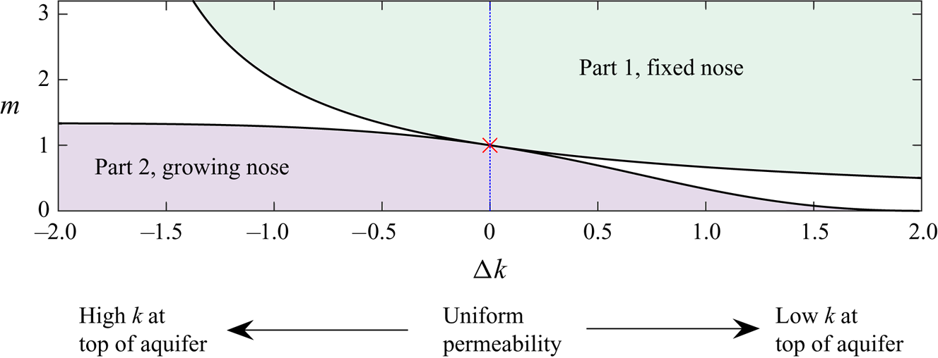
Figure 1. Parameter space from Hinton & Woods (Reference Hinton and Woods2018) for the late-time evolution of the interface between the injected and ambient fluids in the case of linearly varying permeability. The vertical axis corresponds to the viscosity ratio,  $m$, whilst the horizontal axis shows the permeability difference between the top and the bottom of the aquifer ( ${\rm \Delta} k >0$ refers to permeability increasing towards the bottom of the aquifer). For a low viscosity injectate, the interface grows in proportion to time, $t$ (bottom left zone). The migration of tracer in this case is studied in the present paper (Part 2). In the top right region, the interface has fixed extent and the tracer transport in this case was studied in Part 1 (Hinton & Woods Reference Hinton and Woods2020). In the intermediate regions (coloured white) the interface has growing regions and fixed regions. For equally viscous fluids in a uniform aquifer, the interface grows in proportion to $t^{1/2}$ (red cross).
The migration of tracer in the case of a growing nose is characterised by the flow carrying tracer into continually thinner regions of the nose (see figure 2). Hinton & Woods (Reference Hinton and Woods2019) examined the dispersal of a material line of tracer in an aquifer with vertically varying permeability in the case that diffusion is neglected and the migration of the tracer is assumed to be controlled by the advection of the buoyant fluid. They found that the tracer enters the nose region and follows a complex path through the head of the flow. They studied how the first arrival time of tracer at an observation well is influenced by the interface structure and any permeability contrast.
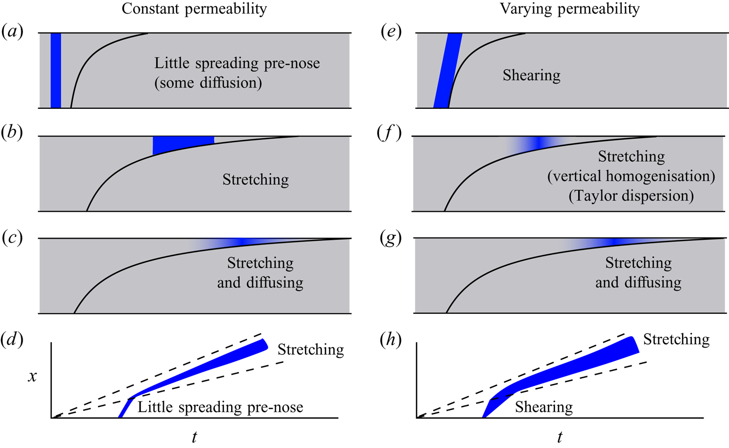
Figure 2. Schematics of the regimes for the migration of tracer in a growing nose. (a–c) The spreading in an aquifer with constant permeability, studied in § 3. A finite-width pulse experiences little dispersion prior to entering the nose. In the nose, it disperses owing to the stretching from the growth of the nose. At very late times, the combination of stretching and diffusion is important and the tracer is diluted. (e–g) Tracer diffusion in an aquifer with vertically varying permeability (§ 4). The shear is important before tracer becomes vertically homogenised. Subsequently, tracer occupies a thin region of the nose and behaves as if the permeability were constant. Taylor dispersion may play a role if the tracer becomes vertically homogenised before it is in very thin regions. (d,h) The location and extent of the tracer pulse relative to the nose (dashed lines).
In the present paper, we consider the dispersal of a finite-width pulse of tracer. When the pulse is in the growing nose, its extent increases in time as the fluid within the nose is vertically squashed and laterally stretched. In the absence of any diffusion, the volume of the pulse of tracer remains constant but its lateral extent increases owing to advection, even in a uniform aquifer. At late times, the lateral extent of the tracer is proportional to  $t^{1/2}$ owing to the growth of the nose. We show that until very late times, diffusion is insignificant in comparison to the stretching in the nose in dispersing the tracer. However, at late times, there is an interesting regime that occurs in which the processes of stretching and diffusion are both important. Each process acts to spread the tracer at the same rate but the diffusion dilutes the tracer into the surrounding fluid, which enhances the stretching and the late-time lateral extent is proportional to $(t \log t)^{1/2}$.
In the case that the aquifer has vertically varying permeability, the combination of a shear flow and cross-flow pore-scale dispersion can enhance the along-flow rate of dispersion. The effect is known as ‘shear dispersion’ and was first identified for Poiseuille flow in a tube (Taylor Reference Taylor1953; Aris Reference Aris1956). This phenomenon may arise in porous media owing to the combination of cross-aquifer heterogeneity, which creates a shear flow, and pore-scale dispersion (Dagan Reference Dagan2012; Woods Reference Woods2015). However, curiously the role of such shear dispersion diminishes as tracer migrates into continually thinner regions of the nose where it samples less of the cross-flow permeability gradient. At such times, the stretching dominates the spreading as in a uniform aquifer (see figure 2e,f). However, the tracer extent in the stretching regime depends on the pre-stretching extent, which is sensitive to the early shearing. Thus heterogeneity can have an important influence even after tracer is in the thin regions of the nose.
As in Part 1, our approach is to develop an idealised model so that we can identify the interaction between the shearing of tracer produced by the heterogeneity and the stretching of tracer produced by the nose. Although it is idealised, the qualitative and quantitative understanding of the structure of the flow field and its influence on the distribution of a pulse of additive as a function of time provides insight into the potential learnings from tracer tests about the aquifer structure. The models also identify how capsulated chemically active agents, which only become active after a time delay may be used to influence the flow near the leading edge of the front even if injected at late times. Since CO $_{2}$ is of very low viscosity, these additives may be deployed ideally to modify the interfacial tension or viscosity at the front.
The present paper is structured as follows. In § 2, we review the model of Hinton & Woods (Reference Hinton and Woods2018) for the evolution of the interface between the fluids. We subsequently introduce the migration of a tracer under advection and diffusion. We consider the release of a vertically uniform pulse of tracer. We then study the case of a nose that grows in proportion to time  $t$ within a uniform aquifer in § 3, corresponding to a low viscosity injectate, and find that tracer migrates into continually shallower regions of the nose where it is stretched owing to the growth of the nose. Next, we study the influence of permeability variations on the dispersion within the growing nose. This creates a shear flow, which leads to shear dispersion but as tracer migrates into thinner regions of the flow, the influence of the shear diminishes. However, the shearing has a strong influence on the lateral extent in the stretching regime. We conclude with some applications of the modelling to tracer tests and the use of viscosifiers in § 5. In appendix A, we study how the tracer migrates within a nose that grows in proportion to $t^{1/2}$, which occurs in the special case of equally viscous fluids in an aquifer of constant permeability.
2. Formulation
In this section, we describe the flow in the case that the nose grows in time, which occurs provided that the input fluid is of low viscosity (see figure 1). The analysis has been carried out in the case that the interface is sharp by Hinton & Woods (Reference Hinton and Woods2018). In § 2.1, we formulate a new model for the advection and diffusion of tracer within the injectate.
Buoyant fluid, of viscosity  $\mu _i$, is injected at a constant rate, $Q$ into a confined aquifer, initially filled with liquid of viscosity $\mu _a$ (figure 3). The aquifer has porosity $\phi$ and permeability $K(Y)$. We scale the spatial coordinates and time using the following relations:
 \begin{equation} h=H/H_0, \quad x = X/H_0, \quad y=X/H_0, \quad t = QT/(\phi H_0^{2}). \end{equation}
We use capital letters to denote dimensional quantities and lower case for dimensionless quantities, with the exception of the density, the viscosity and gravity,  $g$. The dimensionless permeability is $k(y) = K(Y)/\bar {K}$, where $\bar {K}$ is the mean permeability. The viscosity ratio is $m=\mu _i/\mu _a$.
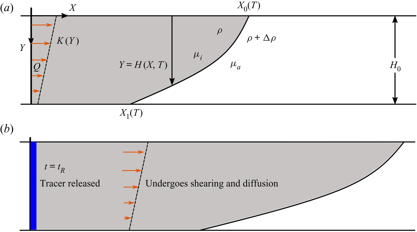
Figure 3. (a) Schematic for the injection of buoyant fluid into a confined aquifer with a vertically varying permeability. (b) A vertically uniform pulse of tracer is released at a time  $t=t_R$ after injection began. The permeability variation creates a shear flow, which leads to shear dispersion.
As the current becomes long and thin, there can be intermingling of the fluids at the leading edge. However, it has been shown experimentally that the sharp interface assumption is valid away from the leading edge and we adopt this approximation herein (Golding & Huppert Reference Golding and Huppert2010; Pegler et al. Reference Pegler, Huppert and Neufeld2014).
In the case of a growing interface, the role of buoyancy is negligible at late times and the dimensionless Darcy velocity in the input fluid is (for details, see Hinton & Woods Reference Hinton and Woods2018)
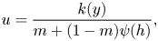 \begin{equation} u = \frac{k(y)}{m + (1-m)\psi(h)}, \end{equation}
where
 \begin{equation} \psi(h) = \int_0^{h} k(y) \,\mathrm{d}y. \end{equation}
The shape of the interface is given implicitly by
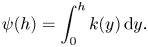
 \begin{equation} x = f'(h) t, \end{equation}
where
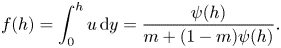 \begin{equation} f(h) = \int_0^{h} u \,{\textrm{d}}y = \frac{\psi(h)}{m + (1-m)\psi(h)}. \end{equation}
Figure 4 shows an example of the evolution of such a nose.
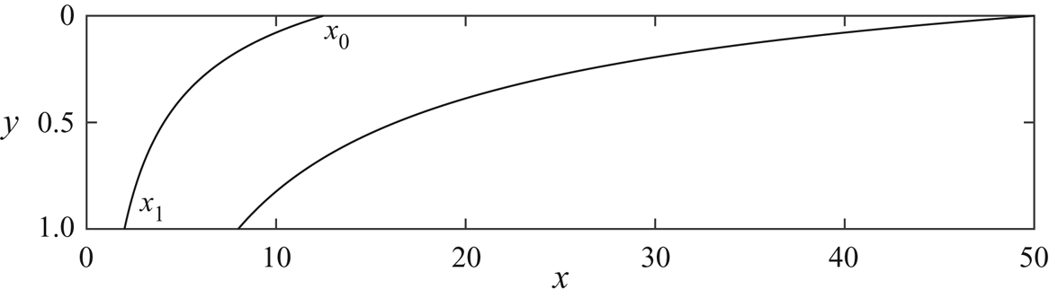
Figure 4. Position of the fluid–fluid interface at  $t=5$ and $t=20$ according to the late-time solutions found by Pegler et al. (Reference Pegler, Huppert and Neufeld2014) and Hinton & Woods (Reference Hinton and Woods2018). The leading and trailing contact points are labelled $x_0$ and $x_1$, respectively. The interface grows in proportion to time $t$. We use $m=0.4$ and a uniform aquifer.
Huppert & Woods (Reference Huppert and Woods1995) showed that in the special case of equally viscous fluids ( $m=1$) in a uniform aquifer, the interface travels downstream with constant velocity whilst extending at a rate proportional to $t^{1/2}$. The migration of tracer in this case is considered in appendix A.
2.1. Migration of tracer
We consider a passive tracer released into the input fluid. The tracer undergoes diffusion with coefficient  $D$. In the case of low flow rates, molecular diffusion is the dominant dispersive mechanism Bear (Reference Bear1961). Hence the diffusion coefficient, $D$, is everywhere a constant. We focus on this situation in the present paper.
We scale the concentration of tracer,  $C$, with the initial concentration so that $0 \leq c \leq 1$. Mass conservation of the tracer leads to the following constraint:
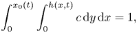 \begin{equation} \int_0^{x_0(t)} \int_0^{h(x,t)} c \,{\textrm{d}}y \,{\textrm{d}}x = 1, \end{equation}
where the current lies in  $0<y<h(x,t)$ and $0<x<x_0(t)$ (see figure 4). The dimensionless advection–diffusion equation is
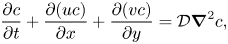 \begin{equation} \frac{\partial c}{\partial t} + \frac{\partial (uc)}{\partial x} +\frac{\partial (vc)}{\partial y} = \mathcal{D} \boldsymbol{\nabla}^{2} c, \end{equation}
where
 \begin{equation} \mathcal{D} = \frac{\phi D}{Q} \end{equation}
is the dimensionless diffusion coefficient. Note that this is the inverse of the Péclet number,  $\mathcal {D}= {Pe}^{-1}$.
Since the flow is incompressible,  $\pmb {\nabla } {\cdot } \pmb {u} = 0$, we can calculate the vertical velocity from the horizontal velocity (2.2),
 \begin{equation} v= - \int_0^{y} \frac{\partial u}{\partial x} \,\mathrm{d}y, \end{equation}
and the condition  $v(y=0)=0$ as there is no flux across the upper boundary. The vertical velocity, $v$ is small in comparison to the horizontal velocity, $u$ because the interface is long and thin at late times. Thus, the assumption of hydrostatic pressure is valid.
We assume a vertical line of non-reacting, non-adsorbing tracer is released into the current from the injection well at a time  $t=t_R$, which is sufficiently long after the injection began so that the late-time regime has developed. The initial concentration of tracer is vertically uniform. We assume that the tracer is immiscible in the ambient fluid; in the context of CO $_{2}$ sequestration, MacMinn, Szulczewski & Juanes (Reference MacMinn, Szulczewski and Juanes2011) showed that the fraction of the CO $_{2}$ that dissolves during the injection period is negligible because of the low solubility of CO $_{2}$ in water.
We assume that the injection of fluid continues at a constant rate throughout the period in which we study the migration of tracer. The evolution of the interface and hence the flow field is significantly altered in the post-injection regime (Hesse et al. Reference Hesse, Tchelepi, Cantwel and Orr2007; MacMinn et al. Reference MacMinn, Szulczewski and Juanes2011). The post-injection migration of tracer is beyond the scope of this paper.
The migration of the tracer in a growing nose in a heterogeneous aquifer is complex. Many physical processes are involved including the shear flow associated with permeability variation, cross-flow diffusion, streamwise diffusion and the interaction with the extending nose. We split the analysis in two. First, in § 3, we consider the migration of tracer in a growing nose in a uniform aquifer. Then in § 4, we develop the model to account for the shear associated with a vertically varying permeability.
3. Dispersion of a tracer pulse in a uniform aquifer
In this section, we study the dispersion of tracer in the case that the interface grows in proportion to time,  $t$ in an aquifer with constant permeability. This occurs when the injected fluid is less viscous than the ambient fluid ( $m <1$). We first consider the dispersion owing to the growth of the nose in the absence of diffusion in § 3.1. Hinton & Woods (Reference Hinton and Woods2019) analysed the migration of a material line of tracer with zero thickness. We show that a pulse with finite thickness disperses within the nose owing to the differing velocities across the lateral extent of the pulse. Next, the role of diffusion is studied in § 3.2.
3.1. Dispersion in the case of zero diffusion
In a uniform aquifer, the interface shape is (see (2.4))
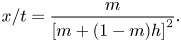 \begin{equation} x/t = \frac{m}{\left[m+(1-m)h \right]^{2}}. \end{equation}
The trailing contact point is at  $x_1(t)=mt$ and the flow velocity upstream of this point is $1$. The time at which tracer enters the nose is thus
 \begin{equation} t_E = \frac{t_R}{1-m}. \end{equation}
The growing region of the current is supplied by fluid from upstream and eventually all the tracer migrates into the growing nose. The horizontal velocity in the nose region is (see (2.2))
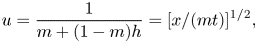 \begin{equation} u = \frac{1}{m+(1-m)h} = [x/(mt) ]^{1/2}, \end{equation}
where we have used our expression for the shape of the interface (3.1). We can use (3.3) to obtain the along-channel position of a particle,
 \begin{equation} x(t) = \left[ \left(\frac{t}{m} \right)^{1/2} - a_0\right]^{2}, \end{equation}
where the constant  $a_0$ is obtained from the entry time (3.2),
 \begin{equation} a_0 = t_E^{1/2}\left(m^{-1/2} -m^{1/2}\right). \end{equation}
The expression for the particle position (3.4) demonstrates that the distance between two particles within the nose increases in proportion to  $t^{1/2}$. If a finite pulse of tracer is released, beginning at $t=t_R$ and stopping and $t=t_R+{\rm \Delta} t$, and ${\rm \Delta} t \ll t_R$ then the tracer extent is a constant, ${\rm \Delta} t$, before entering the nose and after entering the nose ( $t>t_E$) the extent is
 \begin{equation} {\rm \Delta} t \left\{1 + (1/m) \left[ (t/t_E)^{1/2} -1 \right] \right\}. \end{equation}
The tracer disperses longitudinally within the nose as shown in the left-hand column of figure 5. We call this growth within the nose the ‘stretching’ regime. The concentration of tracer is constant because there is no diffusion. Instead the longitudinal spreading arises from the vertical squashing and longitudinal stretching of the fluid in the growing nose. For large times, the extent grows in proportion to  $l_0 (t/t_E)^{1/2}$ where $l_0$ is a constant that is proportional to the initial extent. We plot the lateral extent of the tracer for three release times with $m=0.2$, ${\rm \Delta} t =0.5$ in figure 6(a). For smaller release times, the tracer quickly enters the nose where it disperses. Hence for smaller release times, the tracer spends longer in the nose and thus disperses for longer as a proportion of its travel time and this appears as a higher effective dispersivity (see figure 6b,c).
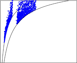
Figure 5. The positions of 1000 particles migrating within the growing nose in a uniform aquifer in the case of zero diffusion ( $\mathcal {D}=0$, left-hand column) and the case $\mathcal {D} > 0$ (right-hand column). For details of the numerical technique, see § 3 of Hinton & Woods (Reference Hinton and Woods2020). (a–e) Particles migrate into shallower regions of the nose and the lateral extent grows in proportion to $t^{1/2}$ owing to advection (see (3.7)). We call this the ‘stretching’ regime. (f) With $\mathcal {D}=0$, the volume of fluid ahead of the tracer is fixed and hence tracer never reaches the leading contact point. (g–k) Diffusion does not alter the qualitative behaviour of the tracer dispersion until very late times. (l) At much later times, tracer reaches the leading contact point (owing to the $t \log t$ dispersion), which acts as a no-flux boundary to the spreading. The tracer subsequently disperses in self-similar fashion with $x\sim (t \log t)^{1/2}$, owing to the combination of advection and diffusion, as described in § 3.
Figure 6. The stretching of tracer owing to the growth of the nose region (zero diffusion). (a) The lateral extent of a pulse of tracer for three release times. Tracer is released during a time interval of  $[t_R, t_R+{\rm \Delta} t]$, we use ${\rm \Delta} t =0.5$ and $m=0.2$. Initially the extent is constant (equal to the initial extent). Tracer subsequently enters the nose and disperses owing to the stretching. For larger release times, the tracer takes longer to enter the nose. (b) The lateral extent of tracer as observed at a well a distance $l=50$ downstream, as a function of release time. The extent is large for small release times because tracer spends longer in the nose. For large $t_R$, the extent converges to ${\rm \Delta} t=0.5$ because tracer never enters the nose. (c) The extent divided by the time for the centre of mass to reach $L=50$. This is a measure of the rate of dispersion. It converges to ${\rm \Delta} t/L=0.01$ as $t_R \to \infty$.
Finally, we calculate how the distance between tracer and the leading contact point of the interface evolves in time. The position of the leading contact point is  $x_0(t) = t/m$. In terms of the distance to the leading contact point, (3.4) can be rewritten as
 \begin{equation} x_0(t) - x(t) = 2a_0 t^{1/2} - a_0^{2}. \end{equation}
The distance grows in proportion to  $t^{1/2}$.
3.2. Role of diffusion in a uniform aquifer
In the previous section, we showed that the flow within the nose leads to the extent of tracer growing in proportion to  $t^{1/2}$. Since this stretching of the flow acts at the same rate as diffusion we anticipate that the combination of stretching and diffusion could lead to an anomalous rate of diffusion and we find that this is the case. The diffusion acts to dilute the tracer concentration and spread tracer beyond the fluid it initially occupies. This diluted tracer distribution continues to be stretched and thus the combination of the two effects – diffusion and stretching – leads to a faster rate of spreading than owing to either process alone.
The distance between particles and the leading contact point grows in proportion to  $t^{1/2}$ owing to the advection (3.7). In the absence of diffusion, tracer cannot reach the leading contact point (figure 5f). However, owing to the combination of stretching and diffusion, tracer disperses more quickly than $(\mathcal {D} t)^{1/2}$ and always reaches the leading contact point (figure 5l).
We anticipate that the combination of advection and diffusion both independently spreading at a rate proportional  $t^{1/2}$ leads to a rate of dispersion asymptotically faster than $t^{1/2}$. Since the rate cannot be a higher power than that owing to diffusion and advection, we conjecture that the lateral extent of tracer evolves in a self-similar fashion with $x \sim (t\log t)^{1/2}$. In appendix B, we formally include the effect of diffusion in the transport equation for the tracer concentration $c$, within the nose and show that this is the case. We find that at late times, tracer interacts with the leading contact point and the depth-integrated concentration profile, $h c$, evolves according to
 \begin{equation} hc = \frac{z}{2 \mathcal{D} t \log (t/t_0)} \exp \left[ \frac{-z^{2}}{4 \mathcal{D} t \log(t/t_0) } \right], \end{equation}
where  $z=t/m - x$ is the distance behind the leading contact point of the nose and $t_0$ is a constant that is determined by comparison with numerical simulations.
We use the expression (3.8) to calculate the distance between the centre of mass of the tracer and the leading contact point. We find this to have value
 \begin{equation} \langle z \rangle = \left[{\rm \pi} \mathcal{D} t \log (t/t_0) \right]^{1/2}. \end{equation}
This contrasts with the distance in the absence of diffusion (3.7) which increases in proportion to  $t^{1/2}$. However, we note that diffusion only plays a dominant role compared to the stretching owing to the growth of the nose when $\mathcal {D} \log t \gg 1$, which corresponds to very late times. Qualitatively, the dispersion is independent of whether there is any diffusion until very late times (compare the columns of figure 5). At times of order $\log t \sim 1/\mathcal {D}$, tracer begins to reach the leading contact point and (3.8) applies.
The along-channel standard deviation is
 \begin{equation} \left(\langle z^{2} \rangle - \langle z \rangle^{2} \right)^{1/2} = \left[(4-{\rm \pi}) \mathcal{D} t \log (t/t_0) \right]^{1/2}, \end{equation}
which is an enhanced rate of dispersion relative to that resulting from diffusion in a constant flow field. Tracer occupies a continually thinner region of the nose near the leading contact point (see figure 5l).
4. Tracer dispersion in an aquifer with vertically varying permeability
We now develop our results to account for the migration of tracer in an aquifer in which the permeability varies vertically and the nose region of the current grows in proportion to time,  $t$. This corresponds to a low viscosity input fluid relative to the ambient. The dispersion of tracer is influenced by four key processes: (i) the shear flow arising from the permeability variation; (ii) cross-flow diffusion, which homogenises the shear flow and leads to Taylor dispersion; (iii) the stretching of the tracer associated with the growth of the nose; and (iv) streamwise diffusion. Our aim in the present section is to determine which combinations of these processes dominate at different times as tracer migrates into continually thinner regions of the growing nose.
Figure 7 shows the evolution of 1000 tracer particles at three times with (a–c)  $\mathcal {D}=0.001$ and with (d–f) $\mathcal {D}=0.004$. We assume that the permeability varies linearly with the vertical coordinate,
 \begin{equation} k(y) = 1 + {\rm \Delta} k (y-1/2), \end{equation}
and in figure 7, we use  ${\rm \Delta} k=-1$. The panels demonstrate that at early times, the shear flow (advection) controls the dispersion. If the tracer is in the nose at these times, the stretching owing to the growth of the nose is also significant. The tracer subsequently becomes vertically well mixed and Taylor dispersion may become important. As the tracer migrates into thinner regions of the nose, the role of Taylor dispersion diminishes. Eventually, the dispersion is as in a uniform aquifer and the anomalous $(t \log t)^{1/2}$ rate of dispersion, owing to the combination of stretching and streamwise diffusion, dominates. In the following subsections, we investigate each of these regimes in turn. We first consider the dispersion prior to the tracer becoming vertically homogenised in § 4.1 and then consider the post-homogenised regime in § 4.2.
Figure 7. The interaction of 1000 tracer particles with a growing nose, released as a vertically uniform pulse at  $t_R=10$ with a linear permeability variation with ${\rm \Delta} k=-1$ and viscosity ratio, $m=0.4$. For details of the numerical technique, see § 3 of Hinton & Woods (Reference Hinton and Woods2020). (a–c) Positions of tracer at three times after release $t-t_R=10,20,50$ for $\mathcal {D}=0.001$. (d–f) Positions of tracer at three times after release $t-t_R=10,20,50$ for $\mathcal {D}=0.004$. The time for vertical homogenisation of the tracer is significantly reduced from $1/\mathcal {D}$ as tracer migrates into thin regions of the nose. The vertical homogenisation is slower with a lower diffusion coefficient. The extent of the tracer is increased with smaller $\mathcal {D}$ because the shear dispersion is inversely proportional to $\mathcal {D}$ (see figure 8).
Note that although we use a linear structure (4.1) for the permeability, the results in the present section apply to any non-uniform permeability variation.
4.1. Advection-controlled dispersion
The dispersion is initially controlled by molecular diffusion in the streamwise direction. However, this quickly becomes negligible in comparison to the shear flow arising from the permeability variation (see figure 7a). Before entering the nose, the tracer extent grows in proportion to time in this pre-homogenisation regime Hinton & Woods (Reference Hinton and Woods2019). The centre of mass migrates at the mean flow velocity,  $1$. The trailing contact point of the nose is at $x= m k(1) t$. The time at which the centre of mass reaches the nose is
 \begin{equation} t_E = \frac{t_R}{1 - mk(1)}. \end{equation}
Within the nose, the stretching driven by the growth of the nose is important as well as the shear flow. This is also an advective process. As tracer migrates into thinner regions of the nose, it samples less of the permeability variation (see figure 7). Therefore, the spreading owing to the shear advection causes the extent of tracer to grow more slowly than  $t$ when tracer is in the nose. Eventually, tracer occupies regions of the nose in which $h \ll 1$ and the influence of the shear becomes negligible in comparison to the stretching owing to the growth of the nose. The dispersion becomes independent of any permeability gradient and the uniform stretching dominates (see § 3).
Cross-aquifer diffusion becomes important at some time. This may occur (a) before tracer enters the nose, (b) after tracer enters the nose and whilst the shear is still important or (c) after the tracer is in very thin regions where the shear is unimportant. The first situation was analysed in Hinton & Woods (Reference Hinton and Woods2020) and tracer becomes homogenised at times of order  $1/\mathcal {D}$. After entering the nose, the homogenisation time is reduced because the vertical extent of the current is less than $1$. In the third situation (c), the description of the dispersion in the present section applies until homogenisation at which point, the permeability gradient is unimportant and the late-time results for a uniform aquifer (§ 3) apply. In appendix C, we show that the time for vertical homogenisation, $t_H$ in this case is proportional to $\mathcal {D}^{-1/2}$. In situation (c), Taylor dispersion never occurs because when the tracer is homogenised, the permeability gradient sampled by the tracer is negligible. In the next section, we investigate the second situation (b) in which homogenisation occurs after entry into the nose but before tracer is in very thin regions (as in figure 7).
4.2. Vertically homogenised tracer
In this section, we study the influence of the permeability variation in tracer dispersion after vertical homogenisation. We investigate how long Taylor dispersion associated with the shear flow is an important mechanism.
When the tracer is homogenised, the role of advection owing to the shear flow diminishes because tracer does not remain in the high (or low) permeability regions but instead it samples the thickness of the flow. Taylor (Reference Taylor1953) showed that the combination of a shear flow and cross-flow diffusion leads to the streamwise extent of tracer growing in proportion to  $t^{1/2}$ but with an enhanced coefficient. The increase in the coefficient is proportional to
 \begin{equation} \frac{{\rm \Delta} u ^{2} h^{2}}{\mathcal{D}}, \end{equation}
where  ${\rm \Delta} u$ is the velocity difference across the flow and in the case of a linear permeability variation, ${\rm \Delta} u={\rm \Delta} k h$.
In figure 8, the streamwise standard deviation of tracer is plotted for  $\mathcal {D}=0.001$ and $\mathcal {D}=0.004$ and ${\rm \Delta} k=-1$. The results are obtained from the numerical method. The situations correspond to those in figure 7. The extent of the tracer is larger for smaller values of $\mathcal {D}$ because the shear extends the tracer further, analogous to Taylor dispersion. The effect of altering $\mathcal {D}$ on the extent of the tracer is complicated because of the complex dependence of the current thickness, $h$, on $\mathcal {D}$ and the dispersion is sensitive to $h$ (4.3). At late times, the stretching in the nose dominates the dispersion and the extent grows in proportion to $t^{1/2}$. We found that decreasing $\mathcal {D}$ from $0.004$ to $0.001$ increased the extent by a factor of $k\approx 1.26$ at late times (see black line in figure 8). Decreased $\mathcal {D}$ leads to a multiplicative increase in the extent because cross-flow diffusion is slower. The case $\mathcal {D}=0$, in which the tracer is never vertically homogenised, is included in figure 8 for comparison.
Figure 8. Lateral standard deviation ( $\sigma$) of the distribution of tracer. Tracer is released as a vertically uniform pulse at $t_R=10$ and there is a linear permeability variation in the aquifer with ${\rm \Delta} k=-1$, viscosity ratio, $m=0.4$. Two values of $\mathcal {D}$ (corresponding to the schematics in figure 7) and the case $\mathcal {D}=0$ are shown. Initially, the dispersion is dominated by the shear and the extent increases in proportion to time, $t$. Once vertically homogenised, the extent grows through stretching which dominates the shear dispersion because tracer is in thin regions. The subsequent growth of the extent is $l_0 (t/t_A)^{1/2}$ to leading order with the constant, $t_A$, corresponding to the time at which the stretching first dominates and $l_0$ is the extent at this time (cf. (3.6)). This is illustrated by multiplying the $\mathcal {D}=0.004$ standard deviation by $k \approx 1.26$ (continuous black line); it shows excellent agreement with $\mathcal {D}=0.001$ at late times. In the limit $\mathcal {D} \to 0$, the tracer never becomes homogenised and the dispersion is controlled by advection owing to the shear, leading to different dispersion. In other words, diffusion acts to slow the dispersion via vertical homogenisation.
For non-zero diffusion, the influence of shear dispersion diminishes at later times because tracer occupies a small fraction of the aquifer (4.3). The dispersion will become dominated by the stretching of the fluid in the nose driven by the growth of the nose.
We illustrate this in figure 9 by comparing the lateral standard deviation of tracer in the case of  $\mathcal {D}=0.004$ and a linear permeability profile (solid blue line) to the same system but with diffusion and the shear set to zero at $t-t_R=50$ and $t-t_R=25$. At such times, the diffusivity is set to zero, the tracer flow velocity is adjusted to its depth-averaged value at each location but the evolution of the interface is unchanged.
Figure 9. Tracer extent for tracer released at  $t_R=10$ with a linear permeability profile ( ${\rm \Delta} k =-1$), diffusivity $\mathcal {D}=0.004$ and viscosity ratio, $m=0.4$. The solid blue line shows the lateral standard deviation of the tracer distribution. The black dashed line shows the standard deviation in the case that we ‘switch off’ the diffusion and the shear flow at a time $t-t_R=50$ and use the depth-averaged horizontal velocity everywhere (the profile at this time is shown in figure 7f). The influence of the shear and shear dispersion is negligible compared to the stretching owing to the growth of the nose and hence the lines agree. For an earlier ‘switch off’ (black dotted-dashed line, $t-t_R=25$), the tracer has not yet vertically homogenised and the shear flow and shear dispersion are still important so the lines diverge.
If we switch off early then the shear associated with the permeability gradient is still important and we underpredict the extent. If we switch off later then stretching dominates and we get same answer as in the case of no switch off. The solid blue line and the black dashed line show excellent agreement because the influence of the permeability gradient and hence the shear is negligible at  $t-t_R=50$. However, for an earlier ‘switch off’ at $t-t_R=25$, the tracer extent grows more slowly in the absence of shear and diffusion because the shear is still important at these earlier times. We can use figure 9 to calculate the time at which the stretching dominates and the aquifer behaves as if it were uniform. Note that the tracer distribution at $t-t_R=50$ is shown in figure 7(f); the tracer is vertically homogenised and in a thin region of the aquifer. The role of the shear flow and shear dispersion is negligible in comparison to the stretching.
Although the tracer dispersion is always dominated by stretching at late times, its extent is sensitive to the earlier shear-controlled spreading as shown in figure 9. This is because the extent of tracer in the stretching regime grows in proportion to  $l_0 (t/t_A)^{1/2}$ where $l_0$ is proportional to the length scale of the tracer extent prior to stretching and $t_A$ is the time at which stretching first dominates (cf. (3.6)). Early shearing enhances the length scale, $l_0$ faster than $t_A^{1/2}$ and hence alters the late-time extent of the tracer pulse despite the shearing becoming dominated by the stretching. This is demonstrated in figure 9.
The final regime for the evolution of the tracer distribution occurs at exponentially late times ( $\log t \sim 1/\mathcal {D}$) when the combination of along-flow diffusion and stretching of the nose occurs and the extent grows in proportion to $(\mathcal {D} t \log t)^{1/2}$ as analysed in § 3.
We note that Hinton & Woods (Reference Hinton and Woods2019) showed that in the absence of diffusion, depending on the viscosity ratio between the input and ambient fluids and the permeability gradient, tracer may enter the nose and migrate into continually thinner regions or tracer may enter the nose but subsequently migrate cross-flow into lower permeability regions and lag behind the advancing nose. For any non-zero  $\mathcal {D}$, the latter, ‘recirculation’ case cannot occur because it requires tracer to migrate through the thinnest regions of the nose where the time for vertical homogenisation tends to zero. Having become vertically homogenised, tracer cannot be recirculated by the permeability gradient.
5. Applications
We consider the implications of our results in the context of CO $_{2}$ storage. We demonstrate how the late-time dispersivity of tracer depends sensitively on the aquifer thickness and any heterogeneity. In a porous medium, we take the coefficient of diffusion of a tracer or solute to be (Woods Reference Woods2015)
 \begin{equation} D = 5 \times 10^{-9}\,\textrm{ms}^{-2}. \end{equation}
We use the following typical values: a viscosity ratio of  $m=0.1$; a porosity of $\phi =0.2$ and an injection flux of $Q=4\times 10^{-5}\,\textrm {m}^{2}\,\textrm {s}^{-1}$ (Boait et al. Reference Boait, White, Bickle, Chadwick, Neufeld and Huppert2012). In a layer of thickness 10 m, the interstitial injection velocity is $V_i=Q/ (\phi H_0) = 2 \times 10^{-5}\,\textrm {m}\,\textrm {s}^{-1}$, a unit of dimensionless time corresponds to approximately six days and the dimensionless diffusion coefficient is $\mathcal {D}=2.5\times 10^{-5}$. Tracer is released one month after the injection began and it is released for a week, which provides the initial length of the pulse.
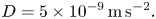
In figure 10(a), the ratio of the lateral standard deviation of the tracer to the along-flow position of the centre of mass of the tracer is plotted as a function of the location of the centre of mass for the 10 m layer. The two cases of an aquifer with constant permeability and an aquifer with linear permeability structure with  ${\rm \Delta} k =-1$ are shown. The extent of the tracer pulse is larger at early times in the heterogeneous aquifer because of the early shearing. The extent is also larger at late times when the tracer has been vertically homogenised and the stretching dominates. This is because the tracer extent in the stretching regime is controlled by the pre-stretching length, which is significantly increased owing to the early shearing.
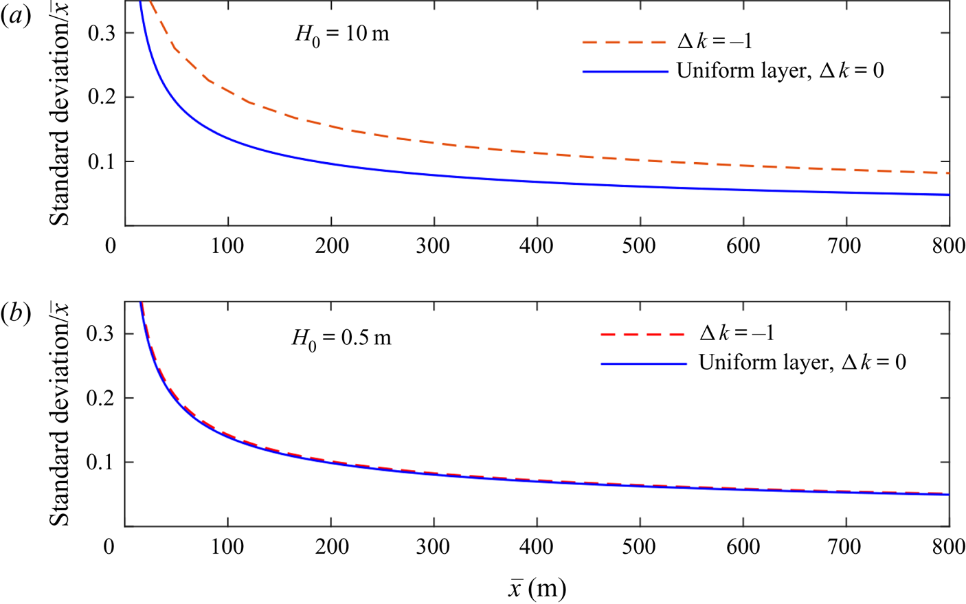
Figure 10. Ratio of the lateral standard deviation of the tracer to the along-flow position of the centre of mass of the tracer as a function of the location of the centre of mass for a uniform aquifer and an aquifer with permeability that varies linearly with depth for two layers of different thicknesses: (a)  $H_0=10$ m and (b) $H_0=0.5$ m. The injection velocity and the other parameters are the same for both layers. The heterogeneity is important in thicker layers but not thinner layers. The results are obtained from the numerical method.
We also consider the dispersion of tracer in a thinner layer with  $H_0=0.5\,\textrm {m}$. We suppose that the injection velocity, $V_i$, is as in the $10\,\textrm {m}$ aquifer. All other parameters are as before and so the dimensionless diffusion coefficient is $\mathcal {D}=5 \times 10^{-4}$. The dispersion of tracer within this layer is plotted in figure 10(b) for ${\rm \Delta} k=0$ and ${\rm \Delta} k =-1$. In contrast to the thick layer, the influence of heterogeneity is negligible. This is because the time for the tracer to become vertically homogenised, and hence the time in which the shearing is important, is much shorter. The stretching extent is approximately independent of the heterogeneity.
These results have profound implications for tracer tests because they demonstrate that heterogeneity has a significant influence on the dispersion in thicker layers, even after tracer is in a thin region of the nose where the permeability is approximately uniform. In addition, the magnitude of this effect increases with layer thickness. In very thin layers the influence of heterogeneity diminishes. Models that treat the subsurface as vertically uniform will likely miss these subtleties and could lead to unrealistic interpretations of tracer tests. Although we have used a linear permeability structure in our calculations, we note that the late-time influence of the early-time shearing owing to the heterogeneity applies to any non-uniform permeability variation and hence this result is quite general. Our results provide a basis for developing techniques to invert the results of tracer tests.
We note that tracer tests last for months or years and the longitudinal diffusive regime in the nose, owing to the combination of stretching and diffusion, is not important at these times.
5.1. Application to chemical additives
The model of the flow in a heterogeneous aquifer identifies that the injection of CO $_{2}$ for sequestration into a saline aquifer, leads to the channelling of the CO $_{2}$ into a relatively thin zone of the reservoir. If an additive is included in the CO $_{2}$ so as to produce a more viscous phase, this will act to deepen the CO $_{2}$ flood and access more of the pore space. Owing to the expense of different chemical systems, it may be that such additives are water soluble, rather than being CO $_{2}$ soluble; using the approach of encapsulation (Yow & Routh Reference Yow and Routh2009) the additives will then become active on reaching the flow front. The present modelling helps to identify and constrain the process by which the shear will enable these additives to approach the leading part of the flow and thereby access the formation water.
6. Conclusion
In this paper we have studied the migration of tracer in the case that the injected fluid is less viscous than the ambient fluid in a uniform aquifer. The nose region grows in proportion to time,  $t$. The flow speed within the growing nose varies in space and time and disperses particles at a rate proportional to $t^{1/2}$ (in the absence of diffusion). We call this novel behaviour the ‘stretching’ regime (see figure 11a). This dispersion is the same rate as that owing to diffusion. The combination of stretching and diffusion within the growing nose leads to an enhanced, anomalous rate of longitudinal dispersion proportional to $(\mathcal {D} t \log t)^{1/2}$ at very late times.
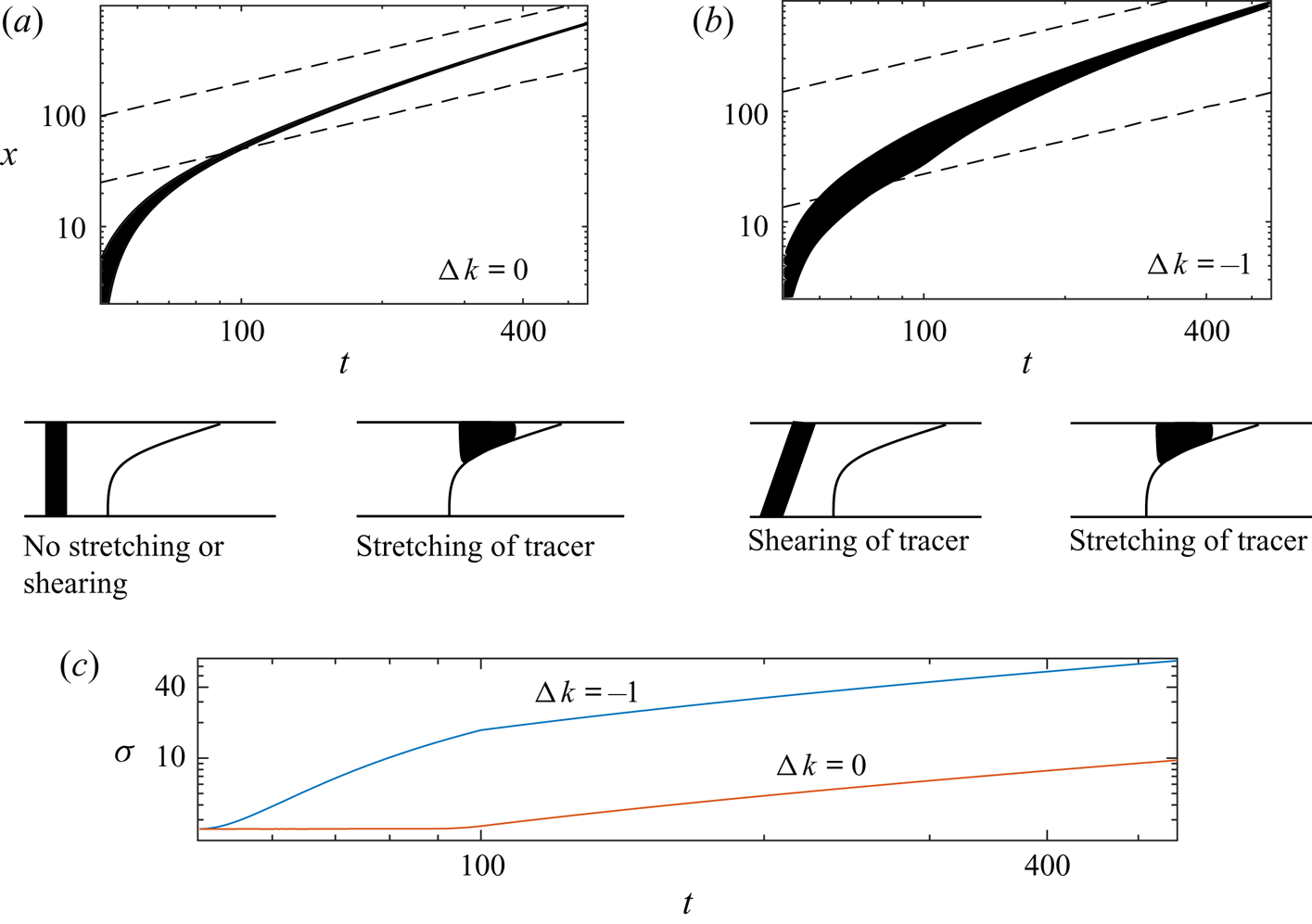
Figure 11. Location of the front of the nose and back of the nose (dashed lines) and the positions of the 10th to 90th percentiles of the tracer distribution in (a) an aquifer with constant permeability ( ${\rm \Delta} k=0$) and (b) an aquifer in which the permeability increases towards the top ( ${\rm \Delta} k=-1$). (c) The lateral standard deviation of the tracer distribution. Prior to entering the nose, the extent is constant in a uniform aquifer (see left most cartoon). The tracer is stretched upon entry into the nose owing to its lateral growth. In a vertically heterogeneous aquifer, tracer is sheared prior to entering the nose. After entering the nose, tracer migrates into thin regions and becomes vertically well mixed. The spreading becomes dominated by the stretching of the nose.
In an aquifer with vertically varying permeability, the nose may still grow in proportion to time provided that the input fluid is not too viscous relative to the ambient. The evolution of the tracer distribution is initially advection controlled and the extent grows in proportion to  ${\rm \Delta} k t$ owing to the shear (see figure 11b,c). At later times, cross-channel diffusion has vertically homogenised the tracer distribution and this leads to an enhanced dispersion coefficient owing to Taylor dispersion (Taylor Reference Taylor1953). However, tracer migrates into continually thinner regions of the nose and the influence of Taylor dispersion becomes negligible as less of the permeability gradient is sampled by the tracer; the late-time migration of tracer is identical to that in a uniform aquifer but with an altered initial condition (see figure 11).
Our results are important for interpreting tracer tests used in CO $_{2}$ sequestration. We have shown that in a typical project, the role of diffusion is important only in homogenising the tracer distribution when it is in a thin region of the nose. The influence of the shear is significant because it controls the extent of tracer in stretching regime. This effect is stronger in thicker layers because the shear acts for longer before vertical homogenisation. Our results also inform the use of additives to alter the viscosity and in particular we have demonstrated how chemicals that are injected at later times end up in thin regions of the growing nose.
In the special case of equally viscous injected and ambient fluids in a uniform aquifer, the nose region grows in proportion to  $t^{1/2}$. Tracer enters the nose and diffuses at the same rate because the advective spreading is much slower than $t^{1/2}$. Therefore, the concentration profile becomes invariant relative to the growing nose.
Acknowledgments
The authors wish to thank T. Espie for his support of this work, and British Petroleum plc and the Engineering and Physical Sciences Research Council for the award of a CASE studentship funding the research.
Declaration of interests
The authors report no conflict of interest.
Appendix A. Nose that grows in proportion to  $t^{1/2}$

We consider the special case of a uniform aquifer in which the injected and ambient fluids have equal viscosity. We note that the tracer is soluble in the injected fluid but not the ambient. Huppert & Woods (Reference Huppert and Woods1995) found that at late times the extent of the nose region grows in proportion to  $t^{1/2}$ and the shape of the interface is a straight line given by
 \begin{equation} h=\frac{1}{2} - \frac{x-t}{2\sqrt{bt}}, \quad \text{for} \ t-\sqrt{bt} \le x \le t+\sqrt{bt}, \end{equation}
where the parameter
 \begin{equation} b=\frac{U_B H_0}{Q} \end{equation}
quantifies the importance of buoyancy relative to injection; the characteristic buoyancy velocity of the injectate is
 \begin{equation} U_B = \frac{{\rm \Delta} \rho g \bar{K}}{\mu_i}. \end{equation}
The leading contact point of the interface is at  $x_0(t) = t+(bt)^{1/2}$. We note that this interface is singular; it is unstable to variations in the viscosity ratio or the permeability structure of the aquifer (Hinton & Woods Reference Hinton and Woods2018).
The flow velocity within the nose incorporates the role of buoyancy, in contrast to the case of a nose that grows in proportion to time  $t$ (Hinton & Woods Reference Hinton and Woods2019),
 \begin{equation} u= 1+\frac{x- [t-(bt)^{1/2}]}{4t}. \end{equation}
In the absence of diffusion, Hinton & Woods (Reference Hinton and Woods2019) showed that the flow carries tracer into continually shallower regions of the nose, and the distance between the tracer and the leading contact point grows in proportion to  $t^{1/4}$. The distance between two particles also grows in proportion to $t^{1/4}$. This is an asymptotically slower rate than diffusive spreading. We anticipate that diffusion will dominate and the extent of the tracer will grow in proportion to $t^{1/2}$, the same rate as the growth of the nose.
The condition of no flux of tracer out of the nose is
 \begin{equation} \frac{\partial c}{\partial y} - \frac{\partial c}{\partial x } \frac{\partial h}{\partial x } = 0 \quad \text{at} \ y=h. \end{equation}
The aquifer is vertically uniform and hence the horizontal flow velocity is independent of depth. Integrating the advection–diffusion equation (2.7) over the thickness of the injected flow yields
 \begin{equation} \frac{\partial c}{\partial t}+ u\frac{\partial c}{\partial x}= \frac{\mathcal{D}}{h} \frac{\partial}{\partial x} \left( h\frac{\partial c}{\partial x}\right). \end{equation}
We transform to a coordinate that grows with the nose:
 \begin{equation} \xi = \frac{1}{2} - \frac{x-t}{2\sqrt{bt}}. \end{equation}
The nose region occupies  $0 \leq \xi \leq 1$ and the depth is $h=\xi$ here. Upstream of this, in $\xi \ge 1$, the depth is $h=1$ and the velocity is $u=1$. The advection–diffusion equation(A 6) is transformed from $(x,t)$ to ( $\xi$, $t$) coordinates as follows:
 \begin{gather} \frac{\partial c}{\partial t} + \frac{1-2\xi}{4t} \frac{\partial c}{\partial \xi} = \frac{\mathcal{D}}{4bt} \frac{\partial^{2} c }{\partial \xi ^{2}} \quad \text{for } 1 \leq \xi \leq \infty \quad \text{(fully flooded region)}, \end{gather}
 \begin{gather}\frac{\partial c}{\partial t} - \frac{\xi}{4t} \frac{\partial c}{\partial \xi} = \frac{\mathcal{D}}{4bt} \xi^{-1} \frac{\partial }{\partial \xi} \left( \xi \frac{\partial c}{\partial \xi} \right) \quad \text{for } 0 \leq \xi \leq 1 \quad \text{(nose region)}. \end{gather}
Both terms on the left-hand side of these two equations are of order  $t^{-1}$, whilst the right-hand sides are $t^{-1}\xi ^{-2}$. The diffusive term scales with the advective term as time increases for fixed $\xi$. This motivates seeking a similarity solution of the form $c=\frac {1}{2}(bt)^{\alpha } g(\xi )$ where $\alpha$ is a constant to be determined using mass conservation. Recasting mass conservation of the tracer (2.6) in the $\xi$ coordinates and substituting in our ansatz for $c$ yields
 \begin{align} 1&=\int_{-\infty}^{t+\sqrt{b t}} h(x,t) c(x,t) \,{\textrm{d}}x = \int_1^{\infty} (bt)^{\alpha} g(\xi) (bt)^{1/2} \,{\textrm{d}} \xi\nonumber\\ &\quad + \int_0^{1} \xi (bt)^{\alpha} g(\xi) (bt)^{1/2} \,{\textrm{d}} \xi, \end{align}
where we split the integral in two because the interface is given by  $h=1$ in $\xi \ge 1$ and, $h=\xi$ in $0\le \xi \le 1$. In order for mass to be conserved, the integrands in (A 10) must have no explicit dependence on $t$ which imposes $\alpha = -1/2$. Upon substituting the ansatz, $c=\frac {1}{2}(bt)^{-1/2} g(\xi )$, into the advection–diffusion equation ((A 8) and (A 9)), we find that the shape function $g$ satisfies
 \begin{gather} -2g + (1-2\xi) g' = (\mathcal{D}/b) g'' \quad \text{for } 1 \leq \xi \leq \infty, \end{gather}
 \begin{gather}-2g - \xi g' = (\mathcal{D}/b) \xi^{-1} (\xi g')' \quad \text{for } 0\leq \xi \leq 1, \end{gather}
with boundary conditions  $g(\infty ) = g'(\infty ) = 0$. These conditions arise because the concentration of tracer decays to zero far behind the nose. This is a result of the transport by the mean flow which continually carries fluid towards the growing nose region. We solve (A 12) by observing that after multiplying by $\xi$, the left-hand side is $-(\xi ^{2} g)'$. Integrating (A 12) twice leads to the half-Gaussian profile
 \begin{equation} g(\xi) = A_0 \exp \left(\frac{-b\xi^{2}}{2\mathcal{D}} \right) \quad \text{for } 0 \leq \xi \leq 1, \end{equation}
where  $A_0$ is a constant of integration that is to be determined. The first constant of integration is set to zero because we assume $c=0$ at the contact point $\xi =0$.
The concentration,  $c$ and its depth-integrated flux, $huc - \mathcal {D} h ({\partial c}/{\partial x})$ are continuous across the trailing contact point $x_1(t)=t-(bt)^{1/2}$ where the linear interface attaches to the bottom boundary of the aquifer. Therefore, $g$ and $g'$ are continuous across $\xi =1$. The solution in the nose region (A 13) provides the boundary conditions for (A 11) at $\xi =1$:
 \begin{equation} g(1) = A_0 \exp(-b/2\mathcal{D}), \quad g'(1) = -\frac{A_0 b}{\mathcal{D}} \exp(-b/2\mathcal{D}). \end{equation}
The initial value problem for the second-order ordinary differential equation (A 11) with initial conditions (A 14) can then be solved for any  $A_0$.
Equation (A 11) can be integrated to obtain
 \begin{equation} (1-2\xi) g = (\mathcal{D}/b) g', \end{equation}
where the constant of integration is zero owing to the condition (A 14). We integrate and apply the boundary condition (A 14) again to obtain
 \begin{equation} g(\xi) = A_0 \exp \left[\frac{b(\xi - \xi^{2} - 1/2)}{\mathcal{D}} \right] \quad \text{for } 1 \leq \xi \leq \infty. \end{equation}
To find  $A_0$, we use mass conservation (A 10), which is
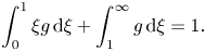 \begin{equation} \int_0^{1} \xi g \,{\textrm{d}} \xi + \int_1^{\infty} g \,{\textrm{d}} \xi = 1. \end{equation}
We obtain
 \begin{equation} A_0 = \left\{ \frac{\mathcal{D}}{b} \left[ 1-\textrm{e}^{-b/2\mathcal{D}} \right] + \textrm{e}^{-b/4\mathcal{D}} \left[ \frac{{\rm \pi} \mathcal{D}}{4b}\right]^{1/2} {\textrm{erfc}} \left[ \sqrt{b/(4\mathcal{D})} \right] \right\}^{-1}. \end{equation}
The full solution can now be calculated numerically and a graph illustrating the variation of  $h g$ with $\xi$ is shown in figure 12 for four values of the relative diffusion coefficient, $d/b$. The function $hg$ corresponds to the concentration integrated over the depth of the nose. We note that in terms of dimensional parameters the relative diffusion coefficient is
 \begin{equation} \mathcal{D}/b = \frac{\phi D}{U_B H_0}. \end{equation}
This is the inverse of the Péclet number associated with the buoyancy velocity,  $U_B$, whereas $\mathcal {D}$ is the inverse of the Péclet number associated with the injection velocity (2.8).
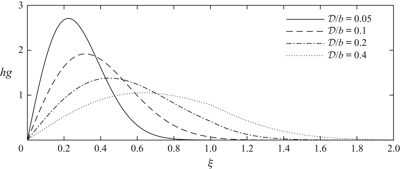
Figure 12. Depth-integrated tracer concentration relative to the growing nose for isoviscous fluids in a uniform aquifer ( $m=1$, ${\rm \Delta} k =0$). The nose of the current occupies $0\leq \xi \leq 1$. The discontinuity in the derivative of $hg$ at $\xi =1$ arises from the discontinuity in the derivative of $h$ at this point.
The self-similar shape of the tracer concentration distribution disperses at the same rate as the nose grows. The diffusive spreading of the tracer and the buoyancy-driven spreading of the nose act at the same rate,  $t^{1/2}$ and their ratio is given by the parameter $\mathcal {D}/b$. The plots in figure 12 indicate that provided $\mathcal {D}/b \ll 1$, almost all of the tracer accumulates in the nose region ( $0 \le \xi \le 1$).
We can interpret these results in real coordinates; the distance from the leading contact point to the centre of mass of the tracer grows in proportion to  $(\mathcal {D} t/b)^{1/2}$ and the standard deviation of the tracer grows at the same rate.
Appendix B. Similarity solution for diffusing tracer in a uniform aquifer
We can formally illustrate the effect of the combination of diffusion and advection within the growing nose by considering the transport equation for the tracer concentration  $c$. First, we transform to the frame moving with the leading contact point, $z=x_0(t) - x$, in which the horizontal velocity is
 \begin{equation} w =\frac{z}{2t} + \mathcal{O}(z^{2}/t^{2}). \end{equation}
We can rearrange (3.1) to obtain the depth to leading order as a function of  $z=t/m -x$ and $t$
$t$
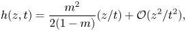 \begin{equation} h(z,t) = \frac{m^{2}}{2(1-m)} (z/t) + \mathcal{O}( z^{2} /t^{2}), \end{equation}
and we note that since tracer migrates into thinner regions of the nose,  $z \ll t$ at late times (cf. (3.7)). In the frame of the leading contact point, $z=t/m - x$, the advection–diffusion equation for the depth-integrated concentration, $ch$ is
 \begin{equation} \frac{\partial (ch)}{\partial t} + \frac{\partial}{\partial z} \left( w c h \right) = \mathcal{D} \frac{\partial}{\partial z}\left( h \frac{\partial c}{\partial z} \right), \end{equation}
where  $w$ is the velocity in the $z$ frame (B 1). The aquifer is vertically uniform and the flow velocity is independent of $y$. Therefore, we have neglected $y$ derivatives (see figure 5).
We can rewrite (B 3) as
 \begin{equation} \frac{\partial (hc)}{\partial t} + w \frac{\partial (hc)}{\partial z} + hc \frac{\partial w}{\partial z} = \mathcal{D} \frac{\partial^{2} (hc)}{\partial z^{2}} -\mathcal{D} \frac{\partial}{\partial z}\left( c \frac{\partial h}{\partial z} \right). \end{equation}
At late times, the tracer is in the thinnest region of the nose and the distance between the tracer and the leading contact point grows much more slowly than the extent of the nose owing to mass conservation as the nose stretches out. Therefore,  $z \ll t$ and we can use the leading-order approximations $w=z/2t$ and $h = \text {const} \times (z/t)$ in the advection–diffusion equation (B 4) to obtain
 \begin{equation} \frac{\partial (hc)}{\partial t} + \frac{\partial}{\partial z} \left(\frac{z}{2t} hc \right) = \mathcal{D} \frac{\partial^{2} (hc)}{\partial z^{2}} - \mathcal{D} \frac{\partial}{\partial z} \left(\frac{hc}{z} \right). \end{equation}
Conservation of mass may be expressed as
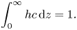 \begin{equation} \int_0^{\infty} h c \,{\textrm{d}}z =1. \end{equation}
 We anticipate that the combination of advection and diffusion both independently spreading at a rate proportional  $t^{1/2}$ leads to a rate of dispersion asymptotically faster than $t^{1/2}$. Since the rate cannot be a higher power than that owing to diffusion and advection, we conjecture that $z \sim (t\log t)^{1/2}$. We seek a self-similar solution to (B 5) and mass conservation condition (B 6) with variables
 \begin{equation} h c = \frac{1}{[\mathcal{D} t \log(t/t_0)]^{1/2}} f (\eta), \quad \eta = \frac{z}{[\mathcal{D} t \log(t/t_0)]^{1/2}}, \end{equation}
where  $t_0$ is associated with the transition time to the similarity solution. It depends on the dispersion at earlier times as tracer migrates further into the nose. Equation (B 5) is recast as an ODE in terms of the similarity variables,
 \begin{equation} -\frac{1}{2} \left(\eta f \right)' = f'' - \left(\,f/\eta \right)', \end{equation}
with mass conservation (B 6) given by
 \begin{equation} \int_0^{\infty} f \,{\textrm{d}} \eta =1. \end{equation}
The solution is
 \begin{equation} f(\eta) = \frac{\eta}{2} \exp\left(\frac{-\eta^{2}}{4} \right). \end{equation}
The constant  $t_0$ in (B 7) is calculated by comparing the similarity solution to the numerical results. In figure 13, we plot both the similarity solution (red dots) and the numerical solutions to the full advection–diffusion equation (B 3) at four times after tracer enters the nose. The numerical results were calculated using MATLAB's PDE solver. With the choice $t_0 =0.7$, the late-time numerical results show good agreement with the similarity solution.
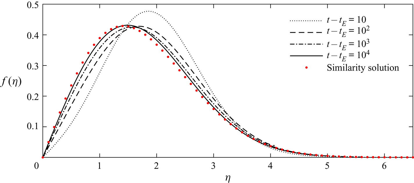
Figure 13. Comparison of the similarity solution and the numerical solutions to (B 3) for the growing nose ( $m<1$). The results are shown in similarity coordinates with viscosity ratio $m=0.5$, diffusion coefficient $\mathcal {D}=1$, and tracer release time $t_R=10$. The numerical results are shown at four times after tracer enters the nose. We chose $t_0=0.7$ to match the late-time numerical results with the similarity solution (B 10).
We use the expression (B 10) to calculate the distance between the centre of mass of the tracer and the leading contact point. We find this to have value
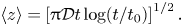 \begin{equation} \langle z \rangle = \left[{\rm \pi} \mathcal{D} t \log (t/t_0) \right]^{1/2}. \end{equation}
Appendix C. Time for vertical homogenisation of tracer in the thin regions of the nose
We calculate an implicit relationship for the evolution of the mean position of the tracer after it is vertically homogenised. The flow velocity in the nose is given by (2.2) with the term owing to buoyancy neglected because the interface has become long and thin,
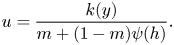 \begin{equation} u = \frac{k(y)}{m + (1-m)\psi(h)}. \end{equation}
Once the tracer is vertically well mixed, the position of the centre of mass of tracer,  $x=\mu (t)$, evolves according to
 \begin{equation} \frac{\mathrm{d} \mu}{\mathrm{d} t} = \frac{1}{h_{\mu}} \int_0^{h_{\mu}} u(\mu,y,t) \,\mathrm{d} y, \end{equation}
where the right-hand side represents the along-channel velocity averaged over the thickness of the nose, which is  $h_{\mu }=h(\mu,t)$. Note that (C 2) is valid even before tracer is vertically well mixed provided that the dispersion is symmetric about the mean (i.e. that tracer has not reached the leading contact point). From (2.5) and (C 1) we obtain
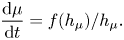 \begin{equation} \frac{\mathrm{d} \mu}{\mathrm{d} t} = f(h_{\mu})/h_{\mu}. \end{equation}
 The shape of the interface is  $x=f'(h) t$ from which we write $\mu =f'(h_{\mu }) t$ and obtain an equation for $h_{\mu }$ alone from (C 3)
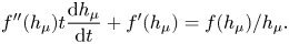 \begin{equation} f''(h_{\mu}) t \frac{\mathrm{d} h_{\mu}}{\mathrm{d} t} + f'(h_{\mu}) = f(h_{\mu})/h_{\mu}. \end{equation}
This can be integrated to obtain
 \begin{equation} \left[f(h_{\mu}) - h f'(h_{\mu})\right] t = t_R, \end{equation}
where we have used the boundary condition of  $h_{\mu }=1$ at $t=t_E$ to determine the constant of integration, $t_R$, which is valid provided that tracer is vertically homogenised before it enters the nose. If this is not the case, (C 5) will be accurate after homogenisation within the nose, but with a different constant of integration (see figure 14).
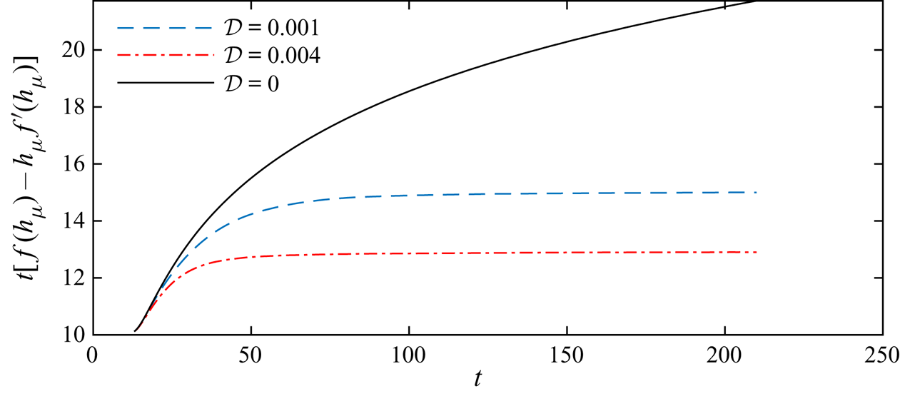
Figure 14. Evolution of the mean horizontal position of tracer plotted using the function on the left-hand side of (C 5) for  ${\rm \Delta} k=-1$, $m=0.4$, $t_R=10$ and two non-zero values of $\mathcal {D}$ (corresponding to the schematics in figure 7) and $\mathcal {D}=0$. The mean position is calculated numerically and then $h_{\mu }$ is the nose thickness at this point. The function converges to a constant after vertical homogenisation and this constant is slightly larger than $t_R=10$ owing to the time for homogenisation. As $\mathcal {D}$ is increased, the constant nears $t_R$.
When  $h\ll 1$, we can use (C 5) to obtain the scaling $h \sim [-f''(0)t]^{-1/2}$. If we assume this is a good approximation even when tracer is not vertically well mixed then we can obtain the homogenisation time by using $t_H \sim h^{2}/\mathcal {D}$, yielding
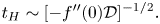 \begin{equation} t_H \sim [-f''(0) \mathcal{D}]^{-1/2}. \end{equation}
This is much faster than the time to homogenise upstream of the nose because tracer is migrating into continually thinner regions.


 Open access