


1. Introduction
Calculating the shape of a sessile drop on a horizontal substrate is a classical problem that goes back to Laplace (Reference Laplace1805). An understanding of that hydrostatic problem is a crucial precursor to the investigation of the transition to dynamical problems, where the drop overcomes static friction and becomes mobile. These problems include sliding (Dupont & Legendre Reference Dupont and Legendre2010), spreading (Hocking & Rivers Reference Hocking and Rivers1982; Eddi, Winkels & Snoeijer Reference Eddi, Winkels and Snoeijer2013) and rolling (Mahadevan & Pomeau Reference Mahadevan and Pomeau1999; Hodges, Jensen & Rallison Reference Hodges, Jensen and Rallison2004).
Owing to axial symmetry, the local force balance at the drop interface may be written as an ordinary differential equation. This nonlinear equation, however, possesses no closed-form solution (Finn Reference Finn1986). The complete mathematical problem governing the drop shape consists of that equation together with appropriate subsidiary conditions. The modern approach for formulating this problem, which reflects experimental protocol, is to specify a fixed drop volume as a constraint (De Gennes, Brochard-Wyart & Quéré Reference De Gennes, Brochard-Wyart and Quéré2003). Upon choosing a characteristic length scale based upon that volume, the dimensionless problem involves only two parameters. The first is the contact angle  $\alpha$, which enters the problem through the triple-line condition. The second is the Bond number $Bo$, reflecting the ratio of gravitational to capillary forces.
For a given contact angle, it is natural to consider the limits of small ( $Bo\to 0$) and large ( $Bo\to \infty$) drops. In the limit $Bo\to 0$, wherein gravity is negligible, the drop shape is a spherical cap (Quéré, Azzopardi & Delattre Reference Quéré, Azzopardi and Delattre1998). In the other extreme, $Bo\to \infty$, the drop adopts a puddle shape where surface tension plays no role except near the edge – a prototype of a singularly perturbed problem (Rayleigh Reference Rayleigh1916; Rienstra Reference Rienstra1990; Van Dyke Reference Van Dyke1994). A simple mechanical description of that limit is provided by De Gennes et al. (Reference De Gennes, Brochard-Wyart and Quéré2003). That limit was additionally described by Quéré (Reference Quéré2005) using an energetic approach, where the constraint of a specified volume was accounted for using Lagrange multipliers.
For fixed  $Bo$, one can inspect the diametric limits of non-wetting drops ( $\alpha =180^{\circ }$) and nearly wetting drops ( $\alpha \ll 1$). Non-wetting drops, approximately realised on superhydrophobic surfaces, were investigated in detail by Aussillous & Quéré (Reference Aussillous and Quéré2006). The present contribution is concerned with the other extreme, of small contact angles. That limit is practically important since it represents the approach to a wetting transition.
The small- $\alpha$ limit was addressed by Dussan & Chow (Reference Dussan V. and Chow1983) as a preliminary step to an investigation of contact-angle hysteresis. In their analysis, Dussan & Chow (Reference Dussan V. and Chow1983) used the contact-line radius as the normalising length scale. While that choice has obvious benefits, it is less appropriate in the modern approach where the drop volume, rather than the contact-line radius, is the specified quantity. Indeed, the formulation of Dussan & Chow (Reference Dussan V. and Chow1983) necessitates the explicit presence of the contact angle in their approximate problem formulation. We discuss the formulation and results of Dussan & Chow (Reference Dussan V. and Chow1983) in § 8.
Our goal here is to address the limit  $\alpha \ll 1$ from the outset using the conceptual approach of De Gennes et al. (Reference De Gennes, Brochard-Wyart and Quéré2003), where both the drop volume and a uniform contact angle are specified.
2. Problem formulation
A sessile drop of density  $\rho$, surface tension $\gamma$ and volume $4{\rm \pi} a^{3}/3$ is placed on a horizontal substrate. The contact angle is $\alpha$. What is the drop shape?
We employ a dimensionless formulation where lengths are normalised by  $a$ and the pressure by $\gamma /a$. We employ cylindrical $(r,z)$ coordinates, with $r=0$ being the symmetry axis and the plane $z=0$ coinciding with the substrate. The contact-line radius is denoted by $r^{*}$. The height of the free surface at the symmetry axis is denoted by $z^{*}$. See figure 1 for an illustrative shape.


The pressure field within the drop is given by the hydrostatic distribution
 \begin{equation} p = p^{*}-Bo\, z, \end{equation}
where  $p^{*}$ is the (as yet unknown) pressure at $z=0$ and
 \begin{equation} Bo = \rho g a^{2} / \gamma \end{equation}
is the Bond number. Using (2.1), the Young–Laplace equation condition at the free surface reads
 \begin{equation} p^{*}-Bo\, z = \boldsymbol{\nabla}\boldsymbol{\cdot}\hat{\boldsymbol{n}}, \end{equation}
wherein  $\hat {\boldsymbol {n}}$ is an outward-pointing unit normal to the surface. This equation is supplemented by: (i) the triple-line condition,
 \begin{equation} \hat{\boldsymbol{n}} = \hat{\boldsymbol{e}}_z \cos \alpha + \hat{\boldsymbol{e}}_r \sin\alpha \quad \text{at}\ z=0, \end{equation}
specifying the contact angle  $\alpha$; (ii) the symmetry condition,
 \begin{equation} \hat{\boldsymbol{n}} = \hat{\boldsymbol{e}}_z \quad \text{at}\ r=0; \end{equation}
and (iii) the volume constraint,
 \begin{equation} \text{dimensionless drop volume} = \tfrac{4}{3}{\rm \pi}. \end{equation}
 It is straightforward to derive an integral force balance in the  $z$ direction,
 \begin{equation} p^{*}{r^{*}}^{2} = \tfrac{4}{3}Bo + 2r^{*} \sin\alpha, \end{equation}
where (2.6) has been used. While this balance does not provide any independent information, it may serve as a convenient alternative to (2.6).
For given  $\alpha$ and $Bo$, the above problem formulation defines the base pressure $p^{*}$ and the drop shape – and in particular the ‘observable’ quantities $r^{*}$ and $z^{*}$. There is no closed-form analytic solution to that nonlinear problem (Finn Reference Finn1986).
3. Numerical scheme
In integrating the Young–Laplace equation (2.3) numerically, it is convenient to start from the apex, where  $r=0$ and $z=z^{*}$. Since $z^{*}$ is unknown to begin with, we employ $\bar {z}= z^{*}-z$ instead of $z$, whereby (2.3) is replaced by
 \begin{equation} p^{**}+Bo\, \bar{z} = \boldsymbol{\nabla}\boldsymbol{\cdot}\hat{\boldsymbol{n}}, \end{equation}
in which the apex pressure  $p^{**}$ remains to be determined.
The free surface is parametrised in the meridian plane using the arclength  $s$, measured from the apex. It is described by a local inclination angle $\phi$, whereby the outward unit vector normal to the surface is (cf. (2.4))
 \begin{equation} \hat{\boldsymbol{n}}=\hat{\boldsymbol{e}}_z\cos\phi+\hat{\boldsymbol{e}}_r \sin\phi. \end{equation}
With  $\boldsymbol {\nabla }\boldsymbol {\cdot }\hat {\boldsymbol {n}}={\textrm d} \phi /{\textrm d} s + r^{-1}\sin \phi$, the Young–Laplace equation (3.1) becomes
 \begin{equation} \frac{{\textrm d} {\phi}}{{\textrm d} {s}} + \frac{\sin\phi}{r} = p^{**}+Bo\, \bar{z}.\end{equation}
Regarding  $r$ and $\bar {z}$ as functions of $s$, they are governed by the differential equations
 \begin{equation} \frac{{\textrm d} {r}}{{\textrm d} {s}} = \cos\phi, \quad \frac{{\textrm d} {\bar{z}}}{{\textrm d} {s}} = \sin\phi. \end{equation}
These first-order equations are supplemented by the ‘initial’ conditions,
 \begin{equation} r(0) = 0,\quad \bar{z}(0)=0, \end{equation}
as well as the symmetry condition (cf. (2.5)),
 \begin{equation} \phi(0)=0. \end{equation}
 The numerical scheme is as follows. For given values of  $Bo$ and $\alpha$, and using an initial guess for $p^{**}$, the preceding initial-value problem is integrated, with a termination at $\phi =\alpha$ (wherein $s$ attains its maximal value, say $s_M$). The violation in the volume constraint (cf. (2.6)),
 \begin{equation} \int_0^{s_M} r^{2}\,\frac{{\textrm d} {z}}{{\textrm d} {s}} \, {\textrm d} s = \frac{4}{3}, \end{equation}
is then used to iterate for  $p^{**}$. Once the iterative scheme converges, we have $r^{*} = r(s_M)$ and $z^{*} = \bar {z}(s_M)$. The advantage of integrating from the apex is the appearance of only one unknown parameter, namely $p^{**}$. (Integration from the contact line would introduce two unknown parameters, namely $p^{*}$ and $r^{*}$.)
The above scheme is illustrated in figure 1, where the drop shape is evaluated for  $\alpha =45^{\circ }$ and $Bo=1$.
4. Small contact angles
Our interest lies in conditions close to perfect wetting,
 \begin{equation} \alpha\ll 1, \end{equation}
considering for now  $Bo$ as arbitrary. It is geometrically evident that the small contact-angle limit (4.1) implies
 \begin{equation} r^{*} \gg 1, \end{equation}
whereby the volume conservation (2.6) necessitates that
 \begin{equation} z^{*} \ll 1.\end{equation}
 For  $\alpha <{\rm \pi} /2$ (and in particular $\alpha \ll 1$) we can write the meniscus shape in the form
 \begin{equation} z = f(r), \end{equation}
where the contact-angle condition (2.4) becomes
 \begin{equation} f'(r^{*}) \approx{-}\alpha \end{equation}
and the symmetry condition (2.5) becomes
 \begin{equation} f'(0) = 0. \end{equation}
Also, from the definition of  $r^{*}$,
 \begin{equation} f(r^{*})= 0, \end{equation}
while the definition of  $z^{*}$ gives
 \begin{equation} z^{*} = f(0). \end{equation}
 With (4.3) implying  $f\ll 1$, the curvature is linearised as (Pozrikidis Reference Pozrikidis2011)
 \begin{equation} \boldsymbol{\nabla}\boldsymbol{\cdot}\hat{\boldsymbol{n}} \approx{-}(\,f'' + f'/r). \end{equation}
Thus, in terms of  $f$, (2.3) becomes
 \begin{equation} p^{*}-Bo\, f \approx{-}(\,f'' + f'/r). \end{equation}
We also observe that, in terms of  $f$, the integral constraint (2.6) reads
 \begin{equation} \int_0^{r^{*}} r f(r)\,{\textrm d} r = \frac{2}{3}. \end{equation}
Lastly, we note the approximated form
 \begin{equation} p^{*}{r^{*}}^{2} \approx \tfrac{4}{3}Bo + 2r^{*}\alpha \end{equation}
adopted by balance (2.7) at small  $\alpha$.
5. Pancake shape
Given (4.2), the linearisation (4.9) suggests that  $\boldsymbol {\nabla }\boldsymbol {\cdot }\hat {\boldsymbol {n}}$ is of order $z^{*}/{r^{*}}^{2} \ll z^{*}$. With the right-hand side of (4.10) being subdominant, we reach an apparent contradiction, since $p^{*}$ is a constant while $f$ must vary (at least) between $0$ and $z^{*}$.
This conflict is resolved by postulating a pancake-like variation, where the interface is approximately flat for most of the range  $0< r< r^{*}$. Thus, $f(r)\approx z^{*}$ except in a narrow ‘edge region’ about $r=r^{*}$ where $f$ must vary between $z^{*}$ and 0. The volume constraint (2.6) then gives
 \begin{equation} {r^{*}}^{2} z^{*} \approx \tfrac{4}{3}, \end{equation}
while the Young–Laplace balance (4.10) in the flat portion gives
 \begin{equation} p^{*} \approx Bo\, z^{*}. \end{equation}
 We therefore have at our disposal two approximate algebraic equations to determine the three unknowns  $p^{*}$, $z^{*}$ and $r^{*}$ without actually solving any differential equations. Since balance (2.7) is not independent, we cannot use it as the requisite third equation. Rather, we employ an integral force balance on half of the drop, in a direction perpendicular to the mid-plane. In the pancake approximation, this gives (cf. De Gennes et al. Reference De Gennes, Brochard-Wyart and Quéré2003)
 \begin{equation} \int_0^{z^{*}} p(z)\,{\textrm d} z \approx 1-\cos\alpha, \end{equation}
independently of the detailed shape of the edge region. Plugging (2.1) into (5.3) and using (4.1) we obtain
 \begin{equation} p^{*}z^{*} - \frac{Bo\, {z^{*}}^{2}}{2} \approx \frac{\alpha^{2}}{2}. \end{equation}
Combining (5.2) and (5.4) gives
 \begin{equation} p^{*} \approx Bo^{1/2}\alpha,\quad z^{*} \approx Bo^{{-}1/2}\alpha. \end{equation}
Then, from (5.1) we obtain
 \begin{equation} r^{*} \approx (4/3)^{1/2}Bo^{1/4} \alpha^{{-}1/2}. \end{equation}
It is readily verified that the force balance (4.12) is trivially satisfied at leading order, with the capillary term being subdominant.
Consider now the edge region. Since the curvature term in (4.10) must enter the dominant balance, we find that this region is of  $\textrm {ord}(1)$ radial extent. Then, (2.4) suggests that $z=\textrm {ord}(\alpha )$ in this region. We therefore write
 \begin{equation} r = r^{*} - x, \end{equation}
so the coordinate  $x$ increases inwards, and express the shape in the form (cf. (4.4))
 \begin{equation} z = \alpha g(x). \end{equation}
Using (4.2) we find that the right-hand side of (4.10) is approximated by the Cartesian curvature  $-\alpha g''(x)$. Making use of (5.5a) we obtain from (4.10) at $\textrm {ord}(\alpha )$
 \begin{equation} g''(x) -Bo\, g + Bo^{1/2} = 0. \end{equation}
This equation is supplemented by the boundary conditions
 \begin{equation} g'(0)=1,\quad g(0) = 0, \end{equation}
which follow from (4.5) and (4.7), respectively, and the matching condition,
 \begin{equation} g(\infty) = Bo^{{-}1/2}, \end{equation}
which follows from (5.5b). The solution of (5.9) and (5.10b) that is bounded at large  $x$ is
 \begin{equation} g(x) = Bo^{{-}1/2} (1-\exp({-Bo^{1/2}x})). \end{equation}
That it trivially satisfies (5.11) is hardly surprising, as (5.2) is equivalent to the balance (5.9) in the absence of the curvature term. Note that (5.12) also satisfies (5.10b). Indeed, (5.5a) has been obtained using the balance (5.3), which has already made use of the contact-angle condition.
6. The distinguished limit  $Bo=\textrm {ord}(\alpha ^{2/3})$

It turns out the pancake approximations (5.5) and (5.6), obtained for arbitrary  $Bo$, agree with the small- $\alpha$ limit of the pancake approximations derived by Quéré (Reference Quéré2005). Since the latter have been obtained for large $Bo$, this is not a priori obvious.
What is more interesting is the breakdown of approximations (5.5) and (5.6) as  $Bo$ becomes small. For $Bo=\textrm {ord}(\alpha ^{2})$ they predict that both $z^{*}$ and $r^{*}$ become $\textrm {ord}(1)$, in contrast to the underlying premise in (4.2) and (4.3). In fact, the breakdown of (5.5) and (5.6) takes place at even larger values of $Bo$: given (5.6), the third term of the integral condition (4.12) is $\textrm {ord}(Bo^{1/4}\alpha ^{1/2})$; it therefore enters the dominant balance of that condition for
 \begin{equation} Bo = \textrm{ord}(\alpha^{2/3}). \end{equation}
In this distinguished limit, both gravity and capillarity play comparable roles.
The transition from dominant gravity to the distinguished limit (6.1) is exemplified in figure 2, showing the numerically evaluated drop shape for  $\alpha =1^{\circ }$ (where $\alpha ^{2/3}\approx 0.0673$) for both $Bo=1$ and $Bo=0.1$. In what follows, we address that limit.

Figure 2. Drop shapes for  $\alpha = 1^{\circ }$, shown for $Bo=1$ and $Bo=0.1$, as produced by the numerical scheme of § 3.
We begin with scaling arguments. The volume conservation (2.6) implies that
 \begin{equation} {r^{*}}^{2} z^{*} = \textrm{ord}(1), \end{equation}
while the definition of  $\alpha$ suggests that (see (4.5))
 \begin{equation} z^{*} = \textrm{ord}(r^{*} \alpha). \end{equation}
Note that, while the volumetric scaling (6.2) is universally valid, the geometric scaling (6.3) holds only when the shape varies over the entire range  $0< r< r^{*}$; in particular, it does not hold in the pancake approximation.
We conclude that
 \begin{equation} z^{*} = \textrm{ord}(\alpha^{2/3}),\quad r^{*} = \textrm{ord}(\alpha^{{-}1/3}). \end{equation}
We accordingly introduce the rescaling
 \begin{equation} z= \alpha^{2/3} \zeta,\quad r = \alpha^{{-}1/3} \eta, \end{equation}
with similar rescaling of  $z^{*}$ and $r^{*}$,
 \begin{equation} z^{*}= \alpha^{2/3} \zeta^{*},\quad r^{*} = \alpha^{{-}1/3} \eta^{*}. \end{equation}
In addition, we express (6.1) in the form
 \begin{equation} Bo = \alpha^{2/3} \beta, \end{equation}
where  $\beta$ is treated as an $\textrm {ord}(1)$ parameter. Since the balance (4.12) now suggests that $p^{*} = \textrm {ord}(\alpha ^{4/3})$, we write $p^{*} = \alpha ^{4/3}\varPhi ^{*}$, where $\varPhi ^{*}$ (which remains to be determined) is treated as an $\textrm {ord}(1)$ parameter.
We now express the shape in the form (cf. (4.4))
 \begin{equation} \zeta = h(\eta), \end{equation}
whereby (4.9) becomes
 \begin{equation} \boldsymbol{\nabla}\boldsymbol{\cdot}\hat{\boldsymbol{n}} \approx{-}\alpha^{4/3} (h''+h'/\eta). \end{equation}
At leading order we obtain from (4.10)
 \begin{equation} h'' + h'/\eta - \beta h + \varPhi^{*} = 0. \end{equation}
This differential equation is subject to two boundary conditions: the first,
 \begin{equation} h'(\eta^{*})={-}1, \end{equation}
follows from (4.5); the second,
 \begin{equation} h(\eta^{*})=0, \end{equation}
follows from (4.7). In addition, the integral balance (4.12) gives
 \begin{equation} \varPhi^{*} {\eta^{*}}^{2} = \tfrac{4}{3}\beta + 2\eta^{*}. \end{equation}
As an alternative to (6.13) we may use the volume constraint (4.11), which now reads
 \begin{equation} \int_0^{\eta^{*}} \eta h(\eta)\,{\textrm d}\eta = \frac{2}{3}. \end{equation}
Once the above problem is solved, we obtain the drop height as (cf. (4.8))
 \begin{equation} \zeta^{*} = h(0). \end{equation}
 The solution of (6.10) and (6.11) that is regular at  $\eta =0$ is
 \begin{equation} h(\eta) = \frac{\varPhi^{*}}{\beta} - \frac{{\mathrm{I}}_0(\beta^{1/2}\eta)}{\beta^{1/2} {\mathrm{I}}_1(\beta^{1/2}\eta^{*})}, \end{equation}
wherein  ${\mathrm {I}}_\nu (R)$ is the modified Bessel function of the first kind and order $\nu$. Substitution of (6.16) into (6.12) gives
 \begin{equation} \varPhi^{*} {\mathrm{I}}_1(\beta^{1/2}\eta^{*}) = \beta^{1/2} {\mathrm{I}}_0(\beta^{1/2}\eta^{*}). \end{equation}
Equations (6.13) and (6.17) serve to determine  $\eta ^{*}$ and $\varPhi ^{*}$ for a given $\beta$. The height $\zeta ^{*}$ is then obtained from (6.15),
 \begin{equation} \zeta^{*} = \frac{\varPhi^{*}}{\beta} - \frac{1}{\beta^{1/2}{\mathrm{I}}_1(\beta^{1/2}\eta^{*})}. \end{equation}
In this scheme, we did not use the volume constraint (6.14).
The approximated drop shape in the distinguished limit (6.1), obtained from (6.5) and (6.8), is portrayed in figure 1 for  $\alpha =45^{\circ }$ (where $\alpha ^{2/3}\approx 0.8513$) and $Bo=1$. It is remarkable that the asymptotic approximation is nearly indistinguishable from the exact numerical solution for this moderate value of $\alpha$. The variation with $\beta$ of $\eta ^{*}$ and $\zeta ^{*}$, as obtained from the transcendental pair (6.13) and (6.17), is portrayed in figure 3.

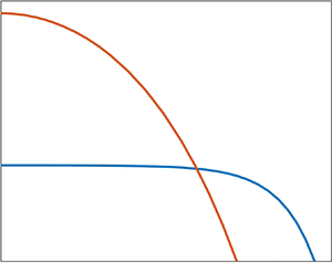
Figure 3. Plots of  $\eta ^{*}$ and $\zeta ^{*}$ as functions of $\beta$. Thick blue lines: solution of (6.13) and (6.17). Thin red lines: pancake limits (6.19). As $\beta \to 0$ the numerical results agree with the approach to the spherical-cap limits $\eta ^{*} = (16/3)^{1/3} \approx 1.7472$ and $\zeta ^{*} = (2/3)^{1/3}\approx 0.8736$; see (6.23) and (6.24).
It is of interest to inspect the limiting forms adopted by the distinguished-limit approximation as  $\beta$ becomes large or small. As $\beta \to \infty$ we find from (6.17) that $\varPhi ^{*}\approx \beta ^{1/2}$ so (6.13) and (6.18) give
 \begin{equation} \eta^{*} \approx (4/3)^{1/2} \beta^{1/4},\quad \zeta^{*} \approx \beta^{{-}1/2}. \end{equation}
Comparing with (5.5b) and (5.6) we find using (6.7) that we have recovered the pancake results, valid for  $Bo\gg \alpha ^{2/3}$.
The other extreme,  $\beta \to 0$, corresponds to $Bo\ll \alpha ^{2/3}$. In that limit, gravity effects perish at leading order in both the local balance (6.10) and the global balance (6.13). It is convenient to address this delicate limit from the outset. Thus, solving the degenerated form of (6.10) and imposing (6.12) together with regularity at $\eta =0$ gives the spherical cap
 \begin{equation} h(\eta) = \tfrac{1}{4}\varPhi{}^{*}({\eta^{*}}^{2}-\eta^{2}). \end{equation}
From condition (6.11) we then obtain
 \begin{equation} \varPhi^{*} \eta^{*} = 2. \end{equation}
 To obtain  $\varPhi ^{*}$ and $\eta ^{*}$, we need another equation. Unlike the general case, we cannot use here the integral balance (6.13); indeed, the degenerated form of that balance (6.13) reproduces (6.21). This was to be expected: with gravity neglected, the volume constraint does not enter that integral balance, which therefore becomes equivalent to the local balance (6.10). We therefore resort to the volume constraint (6.14), which gives
 \begin{equation} \varPhi^{*} {\eta^{*}}^{4} = \tfrac{32}{3}. \end{equation}
The solution of (6.21) and (6.22) is
 \begin{equation} \eta^{*} = (16/3)^{1/3},\quad \varPhi^{*} = (3/2)^{1/3}. \end{equation}
The associated drop height (6.15) is then obtained from (6.20),
 \begin{equation} \zeta^{*} = (2/3)^{1/3}. \end{equation}
Expressions (6.23) and (6.24) agree with the spherical-cap results of Quéré et al. (Reference Quéré, Azzopardi and Delattre1998), when degenerated to small  $\alpha$.
7. Comparison with the numerical solution
The transition from dominant gravity to dominant capillarity is summarised in figure 4, where we show the numerically evaluated  $r^{*}$ and $z^{*}$ as functions of $\alpha$ for $Bo=0.1$ (where the transition angle $Bo^{3/2}\approx 0.0316$). Also shown are the pancake approximations (5.5b) and (5.6) and the spherical-cap approximations (6.6), where $\eta ^{*}$ and $\zeta ^{*}$ are respectively given by (6.23a) and (6.24). Note that the spherical-cap approximations (6.6) break down not only as $\alpha$ approaches the transition value $Bo^{3/2}$ from above, but also as $\alpha$ becomes significantly large so the underlying assumption (4.1) is no longer valid.

Figure 4. Plots of  $r^{*}$ and $z^{*}$ as functions of $\alpha$ for $Bo=0.1$. The thick blue lines are the exact solutions, obtained using the numerical scheme of § 3. The thin red lines provide the pancake approximations (5.5b) and (5.6), valid for $\alpha \ll Bo^{3/2}$. The dashed red lines are the spherical-cap approximations (6.23a) and (6.24), valid for $Bo^{3/2} \ll \alpha \ll 1$.
Figure 4 constitutes the counterpart of figure 10 in Aussillous & Quéré (Reference Aussillous and Quéré2006), showing the transition between different power laws.
8. Comparison with Dussan & Chow (Reference Dussan V. and Chow1983)
At this point it is worth discussing the analysis of Dussan & Chow (Reference Dussan V. and Chow1983). That paper is actually concerned with a sliding drop on an inclined plane, a problem addressed using a lubrication approximation – following Greenspan (Reference Greenspan1978). As a preliminary step to the flow problem, the authors calculated the static drop shape on a horizontal plane in the absence of hysteresis. In that calculation, the radial coordinate has been normalised by the dimensional contact-line radius, say  $R$, while the axial coordinate has been normalised by the product of $\alpha$ with that radius. Denoting these dimensionless quantities by $\tilde {r}$ and $\tilde {z}$, respectively, and writing the drop shape as $\tilde {z} = \tilde {f}(\tilde {r})$, the approximated drop shape obtained by Dussan & Chow (Reference Dussan V. and Chow1983) (see their (2.19)) for small $\alpha$ reads
 \begin{equation} \tilde{f}(\tilde{r}) = \frac{{\mathrm{I}}_0(T^{1/2})-{\mathrm{I}}_0(T^{1/2}\tilde{r})} {T^{1/2}{\mathrm{I}}_1(T^{1/2})}, \end{equation}
wherein  $T=\rho g {R}^{2}/\gamma$ is a Bond number based upon the maximal drop radius, related to $Bo$ via
 \begin{equation} T = Bo\, R^{2}/a^{2}. \end{equation}
 As a consequence of the normalisation scheme in Dussan & Chow (Reference Dussan V. and Chow1983), the volume constraint is not required in evaluating the above approximation. It is required, however, to obtain the dependence of the maximal radius  $R$ upon the drop volume. That constraint reads (see (2.21) in Dussan & Chow (Reference Dussan V. and Chow1983))
 \begin{equation} \frac{\text{drop volume}}{\alpha R^{3}} = \frac{{\rm \pi} {\mathrm{I}}_0(T^{1/2})}{T^{1/2}{\mathrm{I}}_1(T^{1/2})} - \frac{2{\rm \pi}}{T}. \end{equation}
 We now illustrate how these general expressions degenerate to our approximations. In the large-volume limit,  $T\gg 1$, we utilise the large-argument approximations of the Bessel functions to obtain
 \begin{equation} \tilde{f}(\tilde{r}) \approx T^{{-}1/2},\quad \frac{\text{drop volume}}{\alpha R^{3}} \approx {\rm \pi}T^{{-}1/2}. \end{equation}
Making use of (2.6) and (8.2), we find that (8.4) reproduce the pancake approximation (5.5b) and (5.6). When  $\tilde {r}$ is close to 1, (8.4a) is replaced by
 \begin{equation} \tilde{f}(\tilde{r}) \approx \frac{1-\exp({-T^{1/2}(1-\tilde{r})})}{T^{1/2}}, \end{equation}
thus reproducing the near-edge approximation (5.12).
In the small-volume limit,  $T\ll 1$, we utilise the small-argument approximations of the Bessel function to obtain
 \begin{equation} \tilde{f}(\tilde{r}) \approx \frac{1-\tilde{r}^{2}}{2},\quad \frac{\text{drop volume}}{\alpha R^{3}} \approx \frac{\rm \pi}{4}. \end{equation}
Making use of (2.6), we find that (8.6) reproduces the spherical-cap approximation (6.20).
A disadvantage in Dussan & Chow (Reference Dussan V. and Chow1983), which has to do with the choice of  $R$ as a length scale, is the appearance of the contact angle in the volume constraint; see (8.3). This dependence upon $\alpha$ disappears in the distinguished limit (6.1): indeed see (6.4a,b). It is evident that expression (8.1) provides a uniform approximation for all $Bo$ values. (The same is true of the present (6.16).) We prefer to address the pertinent sub-limits of small and large drops separately. This rigorous approach illuminates the under-appreciated condition for the transition between drops and puddles, and provides simple approximations in the pertinent régimes.
9. Concluding remarks
In the absence of hysteresis, the shape of a sessile drop on a horizontal substrate depends upon two parameters,  $Bo$ and $\alpha$. As discussed in § 1, the respective limits of both small and large Bond numbers have been studied extensively. The present investigation, focusing upon $\alpha \ll 1$, provides a complementary analysis to that of Aussillous & Quéré (Reference Aussillous and Quéré2006), who looked at the non-wetting case, $\alpha =180^{\circ }$.
Intuitively, nearly wetting drops appear to suggest a pancake approximation, where capillarity is globally negligible. That approximation, however, breaks down for sufficiently small  $Bo$. That breakdown is represented by the distinguished limit $Bo=\textrm {ord}(\alpha ^{2/3})$, where capillarity becomes comparable to gravity. For $Bo\ll \alpha ^{2/3}$, where gravity is negligible throughout, the drop shape approaches a spherical cap. We note that at the distinguished limit the contact-line radius scales as $Bo^{-1/2}$; see (6.4b). Recalling definition (2.2), this scaling corresponds to a dimensional radius that is comparable to the capillary length $(\gamma /\rho g)^{1/2}$.
In addition to illuminating the limit of small contact angles, the present paper could possibly serve another purpose. Small contact angles are notoriously difficult to measure. It has been suggested (Quéré et al. Reference Quéré, Azzopardi and Delattre1998) that they can be deduced by measuring the maximal drop radius, observed from above. The simple expressions appearing herein for the contact-line radius in the distinct asymptotic sub-limits may be useful for such an in situ measurement.
There are three obvious extensions of the present contribution. The first involves the calculation of the leading-order shape correction, and in particular the leading-order corrections to  $r^{*}$ and $z^{*}$. The second entails more complicated physical mechanisms, such as the presence of electric fields (Mugele & Baret Reference Mugele and Baret2005). The third has to do with the dynamics of spreading puddles (Hocking & Rivers Reference Hocking and Rivers1982), where the asymptotic methodology allows one to quantify the respective roles of meniscus and ‘bulk’ dissipations.
A more ambitious generalisation would involve the calculation of a static shape on an inclined plane. Such a generalisation would require the incorporation of a hysteresis model.
Acknowledgements
I am grateful to the anonymous referee for clarifying the linkage to Dussan & Chow (Reference Dussan V. and Chow1983).
Funding
This work was supported by the Israel Science Foundation (grant no. 2571/21).
Declaration of interests
The author reports no conflict of interest.


 Open access