


1. Introduction
Coherent structures are important for understanding boundary-layer turbulence (Robinson Reference Robinson1991; Schoppa & Hussain Reference Schoppa and Hussain2002; Jiménez Reference Jiménez2018). In the logarithmic region, where the mean streamwise velocity logarithmically depends on the distance to the wall,  $z$, and beyond, various types of coherent motions on a wide range of scales are important for flow dynamics, such as the wall-bounded eddies (Yang, Willis & Hwang Reference Yang, Willis and Hwang2019; Puccioni et al. Reference Puccioni, Calaf, Pardyjak, Hoch, Morrison, Perelet and Iungo2023) and large-scale motions with a streamwise scale of the order of the boundary-layer thickness $\delta$ (Kim & Adrian Reference Kim and Adrian1999; Ganapathisubramani et al. Reference Ganapathisubramani, Hutchins, Hambleton, Longmire and Marusic2005; Hutchins & Marusic Reference Hutchins and Marusic2007; Hutchins et al. Reference Hutchins, Chauhan, Marusic, Monty and Klewicki2012; Sillero, Jiménez & Moser Reference Sillero, Jiménez and Moser2014). These energy-containing motions contribute to the turbulent skin-friction generation (de Giovanetti, Hwang & Choi Reference de Giovanetti, Hwang and Choi2016), and transport of kinetic energy and Reynolds stress (Guala, Hommema & Adrian Reference Guala, Hommema and Adrian2006; Balakumar & Adrian Reference Balakumar and Adrian2007; Wang & Zheng Reference Wang and Zheng2016). The two-point correlation of the fluctuating velocity (Wallace Reference Wallace2014) is widely used to identify the characteristic scales of these coherent structures (Kovasznay, Kibens & Blackwelder Reference Kovasznay, Kibens and Blackwelder1970; Tutkun et al. Reference Tutkun, George, Delville, Stanislas, Johansson, Foucaut and Coudert2009; Bailey & Smits Reference Bailey and Smits2010; Liu, Wang & Zheng Reference Liu, Wang and Zheng2019b). The common practice is obtaining a length scale corresponding to an artificial correlation threshold (Zhou et al. Reference Zhou, Adrian, Balachandar and Kendall1999; Hutchins, Hambleton & Marusic Reference Hutchins, Hambleton and Marusic2005; Dennis & Nickels Reference Dennis and Nickels2011). Liu, Wang & Zheng (Reference Liu, Wang and Zheng2017) summarized the dependence of streamwise, spanwise and wall-normal characteristic length scales on the distance to the wall for varying friction Reynolds number ${Re}_\tau$ in a range of three orders of magnitude. In particular, using a threshold value of $0.05$, the streamwise length scales normalized by $\delta$ show an approximate logarithmic dependence on $z/\delta$. However, this intriguing dependence is empirical and remains to be understood.
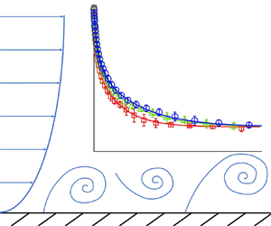
We focus on the two-point correlation of streamwise velocities, i.e. the autocorrelation, with a fixed distance to the wall, illustrated in figure 1. The autocorrelation  $R_{uu}$ relates to the second-order structure function through
 \begin{equation} \langle \Delta
u^2(r) \rangle =\langle
\left[u(\boldsymbol{x}_1+r\boldsymbol{e_x})-u(\boldsymbol{x}_1)\right]^2
\rangle =2 \langle u^2 \rangle
-2\langle u_1u_2 \rangle = 2\langle u^2
\rangle -2R_{uu}(r),
\end{equation}
\begin{equation} \langle \Delta
u^2(r) \rangle =\langle
\left[u(\boldsymbol{x}_1+r\boldsymbol{e_x})-u(\boldsymbol{x}_1)\right]^2
\rangle =2 \langle u^2 \rangle
-2\langle u_1u_2 \rangle = 2\langle u^2
\rangle -2R_{uu}(r),
\end{equation}
where  $u_1=u(\boldsymbol {x}_1)$ and $u_2=u(\boldsymbol {x}_1+r\boldsymbol {e_x})$, with $\boldsymbol {e_x}$ the unit vector in the streamwise direction, are fluctuating velocities at two points with streamwise displacement $r$, and the angular brackets denote the ensemble average. Thus, we can understand the behaviour of autocorrelation based on the existing theories of the second-order structure function $\langle \Delta u^2 \rangle$.

Figure 1. A schematic diagram of the two points in space used for autocorrelation and second-order structure function.
Different ranges of the second-order structure function are discovered in the logarithmic region. In the dissipation range, where  $r$ is of or smaller than the order of the Kolmogorov microscale $l_\nu =(\nu ^3/\epsilon )^{1/4}$ with $\nu$ the viscosity and $\epsilon$ the energy dissipation rate, $\langle \Delta u^2 \rangle \sim r^2$ (Frisch Reference Frisch1995). For scales larger than $l_\nu$, three ranges depicted in figure 2 are defined (cf. Chamecki et al. Reference Chamecki, Dias, Salesky and Pan2017). The inertial range covers the scales between the dissipation scale ( $l_\nu$) and the distance to the wall ( $z$), where Kolmogorov's expression (Kolmogorov Reference Kolmogorov1941) well describes the second-order structure function (de Silva et al. Reference de Silva, Marusic, Woodcock and Meneveau2015). With intermittency considered, Anselmet et al. (Reference Anselmet, Gagne, Hopfinger and Antonia1984) proposed to express $\langle \Delta u^2 \rangle$ as
 \begin{equation} \langle \Delta u^{2} \rangle =C_2 \left( \epsilon r\right) ^{2/3}\left(\frac{r}{l} \right) ^{\xi_2-2/3}, \end{equation}
where  $C_2$ is the Kolmogorov constant, $l$ is a characteristic length scale and the departure of $\xi _2$ from $2/3$ captures the turbulent intermittency (Meneveau & Sreenivasan Reference Meneveau and Sreenivasan1987; She & Leveque Reference She and Leveque1994). de Silva et al. (Reference de Silva, Marusic, Woodcock and Meneveau2015) chose $l=z$, and by introducing the local production-dissipation balance $\epsilon \approx u_\tau ^3/(\kappa z)$ (Pope Reference Pope2000) with $u_\tau$ the friction velocity and $\kappa$ the von Kármán constant, they obtain
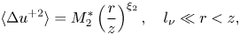 \begin{equation} \langle \Delta u^{+2} \rangle =M_2^*\left(\frac{r}{z} \right) ^{\xi_2},\quad l_\nu\ll r< z, \end{equation}
where the superscript ‘ $+$’ denotes the velocity increment normalized by $u_\tau$ and $M_2^*=C_2 \kappa ^{-2/3}$. For scales larger than $z$ but smaller than the boundary layer thickness $\delta$, the dynamic range, the shear-dominant flow leads to significant anisotropy and $\langle \Delta u^{+2} \rangle$ shows a logarithmic dependence on $r$, i.e. (Davidson, Nickels & Krogstad Reference Davidson, Nickels and Krogstad2006b)
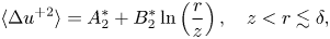 \begin{equation} \langle \Delta u^{+2} \rangle = A_2^*+B_2^*\ln\left( \frac{r}{z} \right) ,\quad z< r\lesssim \delta, \end{equation}
where  $A_2^*$ and $B_2^*$ are constants. The shear production term $-\langle \Delta u\Delta w \rangle \,\mathrm {d} U/\mathrm {d} z$ leads to the logarithmic expression over the scale range from $z$ to $\delta$ (Pan & Chamecki Reference Pan and Chamecki2016; Xie et al. Reference Xie, de Silva, Baidya, Yang and Hu2021). In this range, the pressure-strain-rate correlation is important in the energy redistribution between different velocity components (Ding et al. Reference Ding, Nguyen, Liu, Otte and Tong2018). Additionally, from the perspective of inactive eddies that contribute to streamwise velocity fluctuations but not to the shear stress (Townsend Reference Townsend1961; Marusic & Kunkel Reference Marusic and Kunkel2003; Ding et al. Reference Ding, Nguyen, Liu, Otte and Tong2018), this range can also be called the ‘inactive range’.
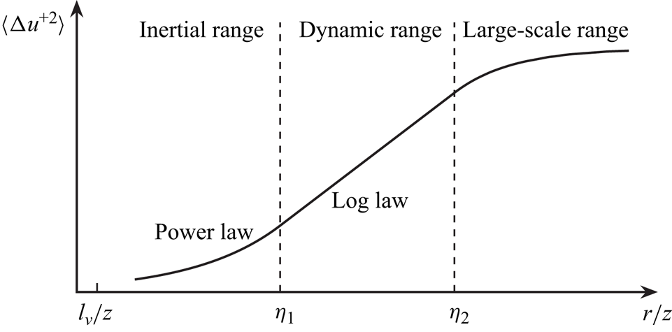
Figure 2. An illustration of the three ranges of the second-order structure function in log-normal coordinates. Here,  $\eta _1$ and $\eta _2$ are the dimensionless lower and upper ends of the dynamic range.
Assuming that there is no distinguished range between inertial and dynamic ranges, Xie et al. (Reference Xie, de Silva, Baidya, Yang and Hu2021) matched the above two ranges at  $r=z$ and determined $A_2^*=M_2^*$ and $B^*_2=M_2^*\xi _2$. In the above analysis, $u_\tau$ captures the characteristic velocity and the characteristic length scale $l$ is chosen to be $z$. In contrast, Davidson & Krogstad (Reference Davidson and Krogstad2014) studied boundary-layer turbulence without local production–dissipation balance and proposed a characteristic length scale $l_\epsilon =u_\tau ^3/\varepsilon$. Pan & Chamecki (Reference Pan and Chamecki2016) extended the use of $l_\varepsilon$ as a characteristic scale to the vegetation canopy where a significant imbalance between local production and dissipation exists. Moreover, Chamecki et al. (Reference Chamecki, Dias, Salesky and Pan2017) investigated the $l_\varepsilon$-dependence in the dynamic range for neutral and stable atmospheric surface layers (ASLs), and obtained the 2/3-power expression for convective ASL turbulence, which is consistent with the $-5/3$ law of spectra predicted by Kader & Yaglom (Reference Kader and Yaglom1989) and Yaglom (Reference Yaglom1994) in the freely convective atmospheric boundary layer and first interpreted by Tong & Nguyen (Reference Tong and Nguyen2015) in convective ASL.
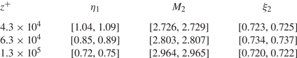
The power and logarithmic expressions in the inertial and dynamic ranges are also obtained for the third-order structure function (Xie et al. Reference Xie, de Silva, Baidya, Yang and Hu2021). Using ASL data measured at the Qingtu Lake Observation Array (QLOA) site, in Minqin District, Gansu Province, PR China, Zhang, Xie & Zheng (Reference Zhang, Xie and Zheng2022) compared the choice of  $l=z$ and $l_\varepsilon =u_\tau ^3/\varepsilon$, and argued that $z$ is also suitable for ASL turbulence with unbalanced energy production and dissipation rate if $u_\tau$ is replaced by $(\varepsilon z)^{1/3}$ as the characteristic velocity scale. In the present work, we do not aim to distinguish the appropriate normalization scale. Following the range division by Chamecki et al. (Reference Chamecki, Dias, Salesky and Pan2017) (cf. figure 2), we choose $u_\tau$ as the characteristic velocity and $z$ as the characteristic spatial scale for structure functions. For convective ASL, the buoyancy effects hold significant importance. This gives rise to another scale range characterized by the $-5/3$ law of spectra (Tong & Nguyen Reference Tong and Nguyen2015; Tong & Ding Reference Tong and Ding2019) and 2/3 power law of second-order structure function (Chamecki et al. Reference Chamecki, Dias, Salesky and Pan2017). We refer to the scales beyond the dynamic range as the large-scale range. Large- and very-large-scale motions that exist in this range have been extensively studied in terms of their contribution to turbulent kinetic energy and Reynolds stress (Balakumar & Adrian Reference Balakumar and Adrian2007; Lee & Sung Reference Lee and Sung2011; Wang & Zheng Reference Wang and Zheng2016). However, the autocorrelation in this range lacks a thorough investigation and is one of the main subjects of the present study.
Several simplified models were proposed since many empirical statistical results have been discovered in boundary-layer turbulence. A notable instance is Townsend's attached eddy model (AEM) (Townsend Reference Townsend1976). In the logarithmic region, the characteristic eddies are assumed to be geometrically self-similar with kinetic energy scales as  $u_\tau ^2$. AEM well captures velocity statistics, such as the logarithmic dependence of the second-order structure function (cf. (1.4)) (Davidson & Krogstad Reference Davidson and Krogstad2014; Yang et al. Reference Yang, Baidya, Johnson, Marusic and Meneveau2017; Xie et al. Reference Xie, de Silva, Baidya, Yang and Hu2021), and it can also describe higher-order statistics after refinement (Marusic & Monty Reference Marusic and Monty2019). In this work, we combine turbulence knowledge, particularly the characteristic scales and the logarithmic expression of structure functions, and time-series statistical methods to explore the global behaviour, which covers the three inviscid ranges, of the second-order structure function.
Several statistical methods have been used to analyse turbulence data obtained in experiments or field measurements as time series, and to perform digital simulation (Di Paola Reference Di Paola1998; Krenk & Møller Reference Krenk and Møller2019) and forecast of wind field velocity (Sfetsos Reference Sfetsos2002; Kusiak, Zheng & Song Reference Kusiak, Zheng and Song2009). Stationary time series can be analysed using the spectral and sequential methods (Kleinhans et al. Reference Kleinhans, Friedrich, Schaffarczyk and Peinke2009; Schmitt & Huang Reference Schmitt and Huang2016; Schmidt et al. Reference Schmidt, Towne, Rigas, Colonius and Brès2018), and often these two are combined. Here we adopt the sequential method because the spectral method is more computationally demanding (Kareem Reference Kareem2008) and because the sequential method yields results directly linked to measured data.
Specifically, we apply an autoregressive moving average (ARMA) model (Shumway, Stoffer & Stoffer Reference Shumway, Stoffer and Stoffer2000), which has broad applicability in engineering applications and theoretical studies of turbulence, particularly in complicated situations where unknown or unresolved impacts may exist. The autoregressive (AR) part of ARMA model assumes that the variable at the current moment is affected by past moments, and the moving average (MA) part models the other unknown effects with a series of noises. For instance, the Langevin equation, which is identical to the first-order AR model, was used to describe the Lagrangian velocities in the inertial range (Thomson Reference Thomson1987). The application of AR and ARMA models for wind field simulation is described by Rossi, Lazzari & Vitaliani (Reference Rossi, Lazzari and Vitaliani2004). In addition, the ARMA model can detect and replace the spikes or outliers in turbulent velocity data due to Doppler noise and signal aliasing (Razaz & Kawanisi Reference Razaz and Kawanisi2011; Dilling & MacVicar Reference Dilling and MacVicar2017). Faranda et al. (Reference Faranda, Dubrulle, Daviaud and Pons2014a,Reference Faranda, Pons, Dubrulle, Daviaud, Saint-Michel, Herbert and Cortetb) tested the applicability of the ARMA model in a turbulent von Kármán swirling flow and remarked that the ARMA model is effective in discriminating different flows. Without prior knowledge, events with undetermined physical mechanisms can be extracted from time series by distinguishing them from the white noise and/or first-order AR process, which, after classification, contributes to the understanding of stable ASL turbulence (Kang, Belušić & Smith-Miles Reference Kang, Belušić and Smith-Miles2014, Reference Kang, Belušić and Smith-Miles2015). Extended AR models for multivariate situations combined with data clustering methods were used to investigate interactions between motions with distinct characteristic scales (Vercauteren & Klein Reference Vercauteren and Klein2015; Vercauteren, Mahrt & Klein Reference Vercauteren, Mahrt and Klein2016; Vercauteren et al. Reference Vercauteren, Boyko, Faranda and Stiperski2019). Moreover, the ARMA model and its combination with other statistical models can be used to analyse and predict non-stationary ASL turbulence (Zhang et al. Reference Zhang, Xie, Chen and Zheng2023).
Our goal is to apply the stochastic equation of the ARMA model to the streamwise velocity series to capture the behaviours of dynamic and large-scale ranges in the logarithmic region of boundary-layer turbulence. Specifically, we aim: (i) to provide a procedure for applying the ARMA model to boundary-layer turbulence; (ii) to provide explanations of parameters in the ARMA model; (iii) to extend the existing theoretical expressions for the second-order structure function to the large-scale range using the analytical expressions based on the ARMA model; and (iv) to explain the behaviour of streamwise characteristic length scales in the logarithmic region and propose an analytical expression that explains experimental and measured data. The ASL data measured from QLOA with high friction Reynolds number ( $Re_\tau \sim O(10^6)$), which could deviate from the typical states of canonical boundary-layer turbulence due to complicated environmental impacts, is used as an example to justify and show the robustness of the obtained expressions.
The rest of this paper is organized as follows. In § 2, we introduce the ARMA model and construct the ARMA model in boundary-layer turbulence. The model application procedure and the analytical expressions are also presented. We present the details of ASL data and perform data analysis and theory verification in § 3. The main results are summarized and discussed in § 4. Appendix A contains the basic properties and details about the ARMA model, and an approximate derivation of the ARMA model parameters leading to the logarithmic expression in the dynamic range is shown in Appendix B. The uncertainty in determining the global expression is discussed in Appendix C.
2. The ARMA model
Although different velocity components are nonlinearly coupled in the Navier–Stokes equation, for model simplicity, we assume the streamwise velocity to be autocorrelated to permit a one-dimensional model. In the context of this paper, ‘autocorrelation’ refers to the correlation function of streamwise velocity evaluated at different times or locations, and we fix the distance to the wall  $z$ located in the logarithmic region. Under these assumptions, we can apply the ARMA model to stationary streamwise velocity time series in boundary-layer turbulence.
For a stationary fluctuating velocity series  $\{u_t\}$, the ARMA( $\kern 0.06em p$, $q$) model is
 \begin{equation} u_t=\sum_{i=1}^{p}\alpha_i u_{t-i\Delta t}+\sum_{j=1}^{q}\beta_j\epsilon_{t-j\Delta t}+\epsilon_t, \end{equation}
where  $p$ and $q$ are the model orders, $\alpha _{i}$ with $i=1,\ldots,p$ and $\beta _j$ with $j=1,\ldots,q$ are the model parameters, $\epsilon _{t-i\Delta t}$ with $i=0,1,\ldots,q$ are independent and identically distributed white noise with variance $\sigma _\epsilon ^2$, $\Delta t$ is the time step, and the subscript $t$ indicates the evaluation time $t$. The maximum model order is referred to as the model's memory depth, which indicates the maximum time range of the current moment to be directly affected. The model applicability and stationarity impose constraints on the model parameters, which are shown with details in Appendix A.
When applying the ARMA model, the orders  $p$ and $q$ and the time step $\Delta t$ should be determined first. In the traditional application of the ARMA model for time series analysis, the corresponding orders are generally empirically determined from the data without known basis (Shumway et al. Reference Shumway, Stoffer and Stoffer2000). If the orders are too small, the data cannot be well fitted; if the orders are too large, more computational effort is needed, which may lead to overfitting. In addition, if the autocorrelation of the data extends over a long time, directly adopting the raw data series with a time step of $\Delta t_0$, which corresponds to the measurement frequency, will result in an excessive number of model orders. In this case, a new time series with a time step $\Delta t>\Delta t_0$ should be resampled from the original series at equal intervals. Overall, there exist uncertainties in the choice of both order and time step of the ARMA model, which requires careful deliberation.
For boundary-layer turbulence, (1.3) and (1.4) present the expressions of streamwise- velocity autocorrelation in the inertial and dynamic ranges, but in the large-scale range, the behaviour of autocorrelation remains obscure. Since the ARMA model provides a global analytical expression for autocorrelation, we attempt to extend the second-order structure-function expression to the large-scale range by modelling the dynamic range with the ARMA model. We focus on the dynamic-range modelling for the following reasons. Since the dominant balances are distinctive in the inertial and dynamic ranges, an ARMA model with a fixed order is not applicable simultaneously in these two regimes. In addition, the large scale separation between the inertial and the dynamic range leads to excessive memory depth of the ARMA model. Therefore, we limit the minimum and maximum time ranges, which correspond to the model orders and the dynamic range of the second-order structure function, respectively. Thus, the autocorrelation has an asymptotically exponential decay in the large-scale range following the ARMA model (see Appendix A, (A13)).
2.1. Constructing the ARMA model in boundary-layer turbulence
The ARMA model applies to a time series, which links to a spatial second-order structure function under Taylor's frozen hypothesis (Taylor Reference Taylor1938). For a measured streamwise turbulent velocity time series with a time step  $\Delta t_0$, mean streamwise velocity $U$ and wall-normal position $z$, we extract a coarse series that does not resolve the small-scale inertial range. So the time step $\Delta t$ of the extracted series satisfies
 \begin{equation} U\Delta t \approx\eta_1 z, \end{equation}
where  $\eta _1$ corresponds to the scale that separates the inertial and dynamic ranges. The new series can be obtained by extracting one point for every $\Delta t/\Delta t_0$ points from the original series.
The larger scale  $\eta _2$ bounds the memory depth of the model, i.e.
 \begin{equation} U\Delta t \max\{p, q\} \approx\eta_1 z\max\{p, q\}\approx\eta_2 z, \end{equation}
where  $p$ and $q$ are undetermined, but at least one of them should equal $\eta _2/\eta _1$. Then in the large-scale range, the autocorrelation (cf. (A13)) takes the form
 \begin{equation} R_{uu}\left(r\right) =\displaystyle\sum_{i=1}^{p}c_i \exp\left(\frac{r}{\Delta x}\ln \lambda_i\right), \quad r\geq\eta_2 z, \end{equation}
with the corresponding second-order structure function
 \begin{equation} \langle \Delta u^2 \rangle =2\langle u^2 \rangle -2\displaystyle\sum_{i=1}^{p}c_i \exp\left(\frac{r}{\Delta x}\ln \lambda_i\right), \quad r\geq\eta_2 z, \end{equation}
where a set of exponential functions approximate the large-scale behaviour of  $\langle \Delta u^2 \rangle$, and $c_i$ and $\lambda _i$ with $i=1,\ldots,p$ are constants related to the model parameters (cf. (A13) and (A14)). In (2.5), a higher order $p$ means the more likely it is to better approximate $\langle \Delta u^2 \rangle$. However, the parameters $c_i$ need to be determined by the autocorrelation of the data, and the roots $x_i$ need to be determined by the model parameters through the fitting procedure. We take a first-order approximation to obtain a more intuitive expression, i.e. $p=1$, then (2.3) leads to $q=\eta _2/\eta _1$. Additionally, the model equation (cf. (2.1)) is reduced to
 \begin{equation} u_t=\alpha u_{t-\Delta t}+\epsilon_t+\sum_{j=1}^{q}\beta_j\epsilon_{t-j\Delta t}. \end{equation}
Here, the velocity  $u$ at the time $t$ depends on the value of $u$ at the previous time $t-\Delta t$ and is subject to random effects with memory depth $q$. The properties of autocorrelation of the ARMA model are presented in Appendix A.
When the two-point displacement is beyond the dynamic range, i.e.  $k>q$, the autocorrelation becomes (cf. (A13))
 \begin{equation} R_{uu}(k\Delta x)=\alpha R_{uu}\left((k-1)\Delta x\right)=\alpha^{k-q}R_{uu}(q\Delta x)=\frac{R_{uu}(q\Delta x)}{\alpha^q}\exp\left(k\ln\alpha\right). \end{equation}
Replacing  $k\Delta x$ with $r$, (2.7) becomes
 \begin{equation} R_{uu}\left(r\right) =\frac{R_{uu}(\eta_2 z)}{\alpha^q}\exp\left(\frac{\ln\alpha}{\Delta x}r\right), \quad r>\eta_2z. \end{equation}
Thus, the autocorrelation implies an exponential decay in the large-scale range since  $\alpha <1$, which is similar to the approximation for correlations in homogeneous turbulence (Taylor Reference Taylor1921; Tennekes Reference Tennekes1979, Reference Tennekes1982).
The AR part of the ARMA model is regarded as the memory effect of flow and mainly controls large-scale motions, and the MA part does not contribute to the large-scale autocorrelation directly. If there is no MA part, the autocorrelation of the ARMA model decays exponentially as the displacement increases. In the dynamic range, the MA part contributes to the autocorrelation (cf. (A9)) and with a further constraint that the MA coefficients follows a power expression with exponent  $-2$, the autocorrelation has a logarithmic dependence on the displacement, which is discussed in Appendix B.
2.2. Linking between ARMA and AEM
Based on the analytical expression of the ARMA model, similar to the AEM, the linear additive form of the MA part in the ARMA model leads to the logarithmic expression. AEM interprets the logarithmic expression of the dynamic range of second-order structure function based on the streamwise velocity representation (Yang et al. Reference Yang, Baidya, Johnson, Marusic and Meneveau2017)
 \begin{equation} u=\sum_{i=1}^{N_z}a_i, \end{equation}
where  $a_i$ is the random velocity increment induced by the attached eddies of size $\delta /2^i$ and $N_z$ is the number of attached eddies contributing to $u$. Namely, the fluctuating velocity $u$ is generated by random eddies with vertical sizes ranging from $z$ to $\delta$, and other potential effects are neglected. Noteworthily, the ARMA model equation (2.1) also contains random variables and the velocity memory. Similar to AEM, we interpret the MA part of the ARMA model as the random effect arising from turbulent eddies. The MA coefficients can be seen as the eddy population density and the random increment $\epsilon$ has the same strength. The above analysis is consistent with the interpretation of the ARMA model by Faranda et al. (Reference Faranda, Pons, Dubrulle, Daviaud, Saint-Michel, Herbert and Cortet2014b) that the AR part is linked to the contribution of the large scales and the MA part corresponds to the effects of eddies and correlation structure. This physical picture also guides us to characterize the dynamic range, from which the model orders are determined.
As mentioned before, the model orders are determined according to the scale information of boundary layers. By Taylor's frozen hypothesis, we can obtain  $\Delta x=U\Delta t$ (cf. (2.2)) and in the ARMA(1, $q$) model, $\Delta x$ is considered as the minimum attached eddy's size, which is of $O(z)$. The memory depth of the model corresponds to the maximum attached eddy's size, $q\Delta x\approx \eta _2 z$, which is of $O(\delta )$ and represents the largest scale of the dynamic range. These scales are also important in AEM. Therefore, the ARMA model can be regarded as a stochastic form of AEM: a set of random white noise, whose scale range is consistent with the sizes of attached eddies, drives the fluctuating velocity. Additionally, in the ARMA model, the MA coefficients $\beta _i$ with $i$ from 1 to $q$ quantify the distribution of attached eddies’ effects (see Appendix B). As shown in figure 8(b) (§ 3.2), the $-2$ exponent in the power function of MA coefficients is consistent with the eddy population density in some AEM studies (de Silva, Hutchins & Marusic Reference de Silva, Hutchins and Marusic2016; Hu, Dong & Vinuesa Reference Hu, Dong and Vinuesa2023). In addition, since the model's stationarity requires $\alpha <1$, the lag term in (2.6) damps this linear dynamical system energized by random noise. Unlike the linear additive process model (cf. (2.9)) proposed for AEM, the ARMA(1, $q$) model hypothetically presents a simple stochastic model of AEM, from which the long-term behaviour of the autocorrelation can be explored. Though Davidson & Krogstad (Reference Davidson and Krogstad2009) provided a general expression for autocorrelation resulting from the attached eddies’ contribution, eddy shape needs to be assumed, and they did not discuss the expression's large-scale behaviour. One advantage of the ARMA model is that the large-scale autocorrelation is obtained without assuming the eddy shape due to the capturing of the memory effect.
2.3. Asymptotic expression of second-order structure function
Even though the ARMA model provides an analytical expression for the second-order structure function in the dynamic and large-scale ranges, this complicated expression is not practically convenient. So in this section, we obtain a global expression covering the inertial, dynamic and large-scale ranges of the second-order structure function by asymptotic matching. As aforementioned, the second-order structure function follows a logarithmic expression in the dynamic range (cf. (1.4)). More generally, in shear flows where the ratio of energy production rate to dissipation rate  $P/\varepsilon$ varies with wall-normal location $z$, which is not rare in ASL turbulence, the two ranges also match at an intermediate scale influenced by $P/\varepsilon$ (Zhang et al. Reference Zhang, Xie and Zheng2022). For the general case, (1.2) becomes
 \begin{equation} \langle \Delta u^{+2} \rangle = \frac{C_2}{\left(\kappa P/\varepsilon \right)^{2/3} } \left(\frac{r}{z} \right) ^{\xi_2} = M_2 \left(\frac{r}{z} \right) ^{\xi_2} ,\quad l_\nu\ll r< z, \end{equation}
where  $M_2$ may be a height-dependent constant due to the presence of $P/\varepsilon$. Assuming that the dimensionless lower and upper ends of the dynamic range are $r/z=\eta _1$ and $r/z=\eta _2$, respectively, we can perform the Taylor expansion on (2.10) and (1.4), and obtain the general form of (1.4) by matching at $r/z=\eta _1$:
 \begin{equation} \langle \Delta u^{+2} \rangle = A_2+B_2\ln\left( \frac{r}{z\eta_1} \right) ,\quad \eta_1< \frac{r}{z}< \eta_2, \end{equation}
where
 \begin{equation} A_2=M_2\eta_1^{\xi_2},\quad B_2=M_2\eta_1^{\xi_2}\xi_2, \end{equation}
and they are obtained by matching (1.3) and (2.11) at  $\eta _1$. The matching process links the dynamic-range coefficients $A_2$ and $B_2$ with the inertial-range coefficients $M_2$ and $\xi _2$, reducing two free parameters. The empirical value of $\eta _1$ is $O(1)$ (Davidson, Krogstad & Nickels Reference Davidson, Krogstad and Nickels2006a; Davidson & Krogstad Reference Davidson and Krogstad2009; de Silva et al. Reference de Silva, Marusic, Woodcock and Meneveau2015; Xie et al. Reference Xie, de Silva, Baidya, Yang and Hu2021), corresponding to a length scale of $O(z)$. For the canonical case, by setting $C_2=2$, $\kappa =0.4$, $\xi _2=2/3$ and $\eta _1=1$, we calculate from (2.12a,b) to obtain $A_2\approx 3.68$ and $B_2\approx 2.46$, whose values are close to previous research (Meneveau & Marusic Reference Meneveau and Marusic2013; de Silva et al. Reference de Silva, Marusic, Woodcock and Meneveau2015; Xie et al. Reference Xie, de Silva, Baidya, Yang and Hu2021).
In § 2.2, the ARMA model is analogous to a stochastic AEM and the attached eddies are modelled as a set of random effects. The logarithmic dependence of  $\langle \Delta u^{+2} \rangle$ can also be obtained from the ARMA model under the assumption of self-similarity with $\beta _{i}\sim i^{-2}$. The details can be found in Appendix B.
In the large-scale range with scales larger than  $\eta _2 z$, conventional AEM does not provide information on the structure functions. The advantage of the ARMA(1, $q$) model is that it naturally provides an exponential autocorrelation for large scales (cf. (2.8)), i.e.
 \begin{equation} \langle \Delta u^{+2} \rangle = 2\langle u^{+2} \rangle -D_2 \exp \left(-E_2 \frac{r}{z} \right) ,\quad \frac{r}{z}>\eta_2, \end{equation}
where  $D_2$ and $E_2$ are positive constants. Assuming that there is no distinguished range between the dynamic and the large-scale ranges, we match the expression in these ranges to determine three unknown parameters $\eta _2$, $D_2$ and $E_2$. By defining $r' = r/z$, we expand (2.11) and (2.13) to
 $$\begin{gather} \langle \Delta u^{+2} \rangle =A_2+B_2\ln\left(\frac{r'_0}{\eta_1}\right) +\frac{B_2}{r'_0}\,\mathrm{d} r' -\frac{B_2}{2r'^2_0}\left(\mathrm{d} r'\right)^2+\cdots,\end{gather}$$
 $$\begin{gather}\langle \Delta u^{+2} \rangle =2\langle u^{+2} \rangle -D_2 \exp\left(-E_2 r'_0 \right) +D_2E_2\exp\left(-E_2 r'_0 \right)\,\mathrm{d} r'\nonumber\\ -\frac{D_2E_2^2}{2}\exp\left(-E_2 r'_0 \right)\left(\mathrm{d} r'\right)^2+\cdots. \end{gather}$$
Matching the leading, the first- and second-order terms at  $r'_0=\eta _2$, we obtain
 $$\begin{gather} D_2=B_2 \mathrm{e}, \end{gather}$$
 $$\begin{gather}\eta_2=\frac{1}{E_2}= \eta_1\exp\left( \frac{2\langle u^{+2} \rangle -B_2-A_2}{B_2}\right). \end{gather}$$
Thus, (2.13) becomes
 \begin{equation} \langle \Delta u^{+2} \rangle =2\langle u^{+2} \rangle -B_2\exp \left(1 - \frac{r}{z\eta_2} \right) ,\quad \frac{r}{z}>\eta_2 . \end{equation}
At the intermediate scale within distinct ranges, the dominant terms exhibit comparable magnitudes, while higher-order terms might also hold significance (Tong & Ding Reference Tong and Ding2019). Here, to obtain a concise expression, we neglect these higher-order terms for simplicity and find that direct matching of low-order terms works well. Equations (2.10), (2.11) and (2.16) constitute the global expression for the second-order structure function, where the coefficients are not all independent. With known turbulent intensity  $\langle u^{+2} \rangle$ and three small-scale parameters $M_2$, $\xi _2$ and $\eta _1$, the global expression for the second-order structure function is determined. For a fixed height, the global expression applied to three horizontal scale ranges is determined by four parameters: $\langle u^{+2} \rangle$, $M_2$, $\xi _2$ and $\eta _1$. Additionally, the height dependence is captured by the logarithmic dependence of $\langle u^{+2} \rangle$, $\langle u^{+2} \rangle =A_1-B_1 \log (z/\delta )$, thus, we have in total five parameters: $A_1$, $B_1$, $M_2$, $\xi _2$ and $\eta _1$.
Assuming that the boundary layer thickness captures the outer scale for large-scale motions, we set the large-scale range's characteristic scale  $\eta _2z$ of $O(\delta )$. In the logarithmic region, the streamwise turbulence intensity follows (Marusic et al. Reference Marusic, Monty, Hultmark and Smits2013; Meneveau & Marusic Reference Meneveau and Marusic2013)
 \begin{equation} \langle u^{+2} \rangle =A_1-B_1\ln \left( \frac{z}{\delta} \right), \end{equation}
where  $B_1$ is the Townsend–Perry constant and $A_1$ is a flow-dependent constant. The size of the attached eddies that contribute to the velocity ranges from $z$ to $\delta$, which is consistent with $\delta$ as the characteristic length scale of the large-scale range. Substituting (2.17) into (2.15b), we get
 \begin{equation} \eta_2=\eta_1 C_\eta \left( \frac{\delta}{z}\right) ^{2B_1/B_2}, \end{equation}
where  $C_\eta =\exp [ ( 2A_1-B_2-A_2 )/B_2]$ and $\eta _1$ is of $O(1)$. Considering a canonical situation with $B_2=2B_1$ (Davidson et al. Reference Davidson, Nickels and Krogstad2006b; Davidson & Krogstad Reference Davidson and Krogstad2014), for example, $B_1=1.25$ (Meneveau & Marusic Reference Meneveau and Marusic2013) and $B_2=2.5$ (Xie et al. Reference Xie, de Silva, Baidya, Yang and Hu2021), we obtain $\eta _2\sim \delta /z$, which is consistent with our analysis and the assumption that $\eta _2z\sim \delta$. Also, rearranging (2.15b), we obtain
 \begin{equation} \langle u^{+2} \rangle =\frac{A_2+B_2}{2}+\frac{B_2}{2}\ln \left(\frac{\eta_2}{\eta_1}\right). \end{equation}
Taking the approximation  $\eta _2/\eta _1\sim \delta /z$, (2.19) recovers the expression for streamwise turbulent intensity (2.17) and $B_2=2B_1$. Even though $B_2$ may not equal twice of $B_1$ in real ASL measurement data, which we show in figure 10(b) (§ 3.3), the assumed exponential expression in the large-scale range links the dynamic range and $r\to \infty$, and is consistent with the matching procedure by Davidson & Krogstad (Reference Davidson and Krogstad2014). The above results show that the proposed exponential function for $\langle \Delta u^{+2} \rangle$ based on the ARMA model is consistent with and bridges previous theories.
2.4. Implication of the global expression
2.4.1. Characteristic length scales calculated from the global expression
In this section, we derive the expression of characteristic length scale from the previously obtained expression of  $\langle \Delta u^{+2} \rangle$. The characteristic length scale $L_x$ is defined by introducing an artificial threshold $T$ of the autocorrelation:
 \begin{equation} R_{uu}(L_x/2)=T \langle u^2 \rangle . \end{equation}
 Though studies show that the threshold value does not change the trend of obtained length scales (Zhou et al. Reference Zhou, Adrian, Balachandar and Kendall1999), we believe the reason is that the threshold values are usually small. The length-scale behaviour could change when different thresholds locate in different ranges of the second-order structure function. For example, the thresholds corresponding to  $\eta _1$ and $\eta _2$ are
 $$\begin{gather} T_{\eta_1}=1-\frac{M_2 \eta_1^{\xi_2}}{2\langle u^{+2} \rangle }, \end{gather}$$
 $$\begin{gather}T_{\eta_2}=\frac{B_2}{2\langle u^{+2} \rangle }. \end{gather}$$
The dependences of  $T_{\eta _1}$ and $T_{\eta _2}$ on $z/\delta$ are shown in figure 3, showing that the detected characteristic length scale depends on the choice of the threshold value, e.g. if $T=0.05$, the threshold locates in the large-scale range, and if $T=0.4$, the threshold locates in the dynamic range.


Taking  $\langle \Delta u^{+2} \rangle =2(1-T )\langle u^{+2} \rangle$ in different ranges of $\langle \Delta u^{+2} \rangle$, we can obtain the analytical expression for the length scale $L_x/\delta$ predicted for different thresholds:
 \begin{align} \frac{L_x}{\delta} =\left\{ \begin{array}{@{}ll} 2\eta_1 C_\eta \left(\dfrac{z}{\delta}\right)^{1-2B_1/B_2}\left\{ 1-\ln\left[ \dfrac{2T}{B_2}\left( A_1-B_1 \ln \left( \dfrac{z}{\delta}\right) \right) \right] \right\} , & T< T_{\eta_2},\\ 2\eta_1\exp \left[ \dfrac{2(1-T)A_1 -A_2}{B_2} \right] \left( \dfrac{z}{\delta} \right)^{1-2B_1(1-T)/B_2}, & T_{\eta_2}< T< T_{\eta_1},\\ 2\dfrac{z}{\delta}\left[ \dfrac{2(1-T)}{M_2}\left(A_1-B_1\ln \left( \dfrac{z}{\delta} \right) \right) \right]^{1/\xi_2} , & T>T_{\eta_1}. \end{array} \right. \end{align}
Since  $\langle u^{+2} \rangle$ is expressed in terms of $A_1$ and $B_1$, there is an extra parameter in the expression for $L_x$ compared with the global expression for the second-order structure function. The main independent parameters that control the behaviour of $L_x$ are $A_1/B_2$ and $B_1/B_2$, and other parameters are close to their canonical value. It is interesting to show that when $T< T_{\eta _2}$, the characteristic length has a double-log dependence on the distance to the wall, which is one of our main results and is checked below by experimental data. Additionally, for a threshold value corresponding to the dynamic and inertial ranges, the behaviours of $L_x$ can also be described by (2.22). If one wants to observe the large characteristic scales corresponding to the flow structure with the dynamics, the threshold value should not be chosen to be greater than the minimum value of $T_{\eta _2}$, as shown in figure 3.
2.4.2. Lower bound for the streamwise turbulent intensity in the logarithmic region
Assuming that the streamwise autocorrelation function decays with increasing scale, which is commonly found in experiments and numerical simulations of boundary-layer turbulence, the value of  $\langle \Delta u^{+2} \rangle$ at $r/z=\eta _2$ should be larger than that at $r/z=\eta _1$ in the dynamic range. Therefore, (2.11) and (2.16) imply
 \begin{equation} 2\langle u^{+2} \rangle -B_2\geq A_2. \end{equation}
With  $A_2=B_2/\xi _2$ and $B_2=C_2\kappa ^{-2/3}\eta _1^{\xi _2}\xi _2$, we obtain
 \begin{equation} \langle u^{+2} \rangle \geq\frac{1}{2}\left(1+\frac{1}{\xi_2}\right)C_2\kappa^{-2/3}\eta_1^{\xi_2}\xi_2. \end{equation}
Taking  $C_2=2$, $\kappa =0.4$, $\xi _2=2/3$ and $\eta _1=1$, we find a lower bound for the turbulence intensity in the logarithmic region $\langle u^{+2} \rangle \geq 3.07$, which is justified by previous results $\langle u^{+2} \rangle$ (Hutchins et al. Reference Hutchins, Chauhan, Marusic, Monty and Klewicki2012; Wang & Zheng Reference Wang and Zheng2016). In addition, this lower bound depends on the imbalance between energy production and dissipation because $\eta _1$ increases as dissipation increases (Zhang et al. Reference Zhang, Xie and Zheng2022). More numerical and experimental results are needed to further check the validity of this lower bound.
2.4.3. Estimation of the integral length scale
Knowing the global expression for second-order structure function, the integral length scale  $\mathcal {L}$ can be calculated as
 \begin{equation} \mathcal{L}=\int_0^{\infty} \frac{\langle u_1u_2 \rangle }{\langle u^2 \rangle }\,\mathrm{d} r =\int_0^{\infty} \frac{\langle u^2 \rangle -\langle \Delta u^2 \rangle /2}{\langle u^2 \rangle }\,\mathrm{d} r =\int_0^{\infty} \left(1-\frac{\langle \Delta u^{+2} \rangle }{2\langle u^{+2} \rangle }\right)\,\mathrm{d} r. \end{equation}
Denoting  $r/z$ as $\eta$, and using (2.10), (2.11) and (2.16), we get
 \begin{align} \frac{\mathcal{L}}{z}&=\int_0^{\infty} \left(1-\frac{\langle \Delta u^{+2} \rangle }{2\langle u^{+2} \rangle }\right)\,\mathrm{d} \eta\nonumber\\ &\approx \int_0^{\eta_1} \left( 1-\frac{M_2 \eta^{\xi_2}}{2\langle u^{+2} \rangle } \right)\,\mathrm{d} \eta +\int_{\eta_1}^{\eta_2} \left[ 1-\frac{A_2+B_2 \ln (\eta/\eta_1)}{2\langle u^{+2} \rangle } \right]\,\mathrm{d} \eta \nonumber\\ &\quad +\int_{\eta_2}^{\infty} \left[ 1-\frac{2\langle u^{+2} \rangle -B_2\mathrm{e}^{1-\eta/\eta_2}} {2\langle u^{+2} \rangle }\right]\,\mathrm{d} \eta \nonumber\\ &= I_1+I_2+I_3. \end{align}
Referring to (2.12a,b) and (2.15b), we can express  $M_2$, $A_2$ and $\eta _2$ as functions of $B_2$, $\eta _1$ and $\xi _2$. Denoting $B_2/(2\langle u^{+2} \rangle )$ as $\mu$, the integrals in (2.26) can be calculated as
 $$\begin{gather} I_1=\int_0^{\eta_1} \left( 1-\frac{\mu \eta^{\xi_2}}{\eta_1^{\xi_2} \xi_2} \right)\,\mathrm{d} \eta = \eta_1-\frac{\mu}{\xi_2 (\xi_2+1)}\eta_1, \end{gather}$$
 $$\begin{gather}I_2=\int_{\eta_1}^{\eta_2} \left[ 1- \frac{\mu}{\xi_2}-\mu \ln \left(\frac{\eta}{\eta_1}\right) \right]\,\mathrm{d} \eta = \left(\frac{\mu}{\xi_2}-1-\mu\right)\eta_1+2\mu \eta_2, \end{gather}$$
 $$\begin{gather}I_3=\int_{\eta_2}^{\infty} \left[ \mu\mathrm{e}^{1-\eta/\eta_2} \right]\,\mathrm{d} \eta = \mu \eta_2, \end{gather}$$
where the second integral uses  $\ln (\eta _2/\eta _1)=1/\mu -1-1/\xi _2$ (cf. (2.15b)). Then we obtain
 \begin{equation} \frac{\mathcal{L}}{z}=-\frac{\xi_2 \mu}{\xi_2+1}\eta_1+3\mu \eta_2. \end{equation}
Again using (2.15b), (2.28) can be further expressed as
 \begin{equation} \frac{\mathcal{L}}{z}=\left[ 3\mu\exp \left( \frac{1}{\mu}-1-\frac{1}{\xi_2}\right) -\frac{\xi_2 \mu}{\xi_2+1} \right]\eta_1=f_1(\mu,\xi_2)\eta_1 \end{equation}
or
 \begin{equation} \frac{\mathcal{L}}{z}=\left[ 3\mu-\frac{\xi_2 \mu}{(\xi_2+1)\exp \left( 1/\mu-1-1/\xi_2\right)} \right]\eta_2=f_2(\mu,\xi_2)\eta_2. \end{equation}
Here, the expressions are reformed to compare with two characteristic scales corresponding to  $\eta _1$ and $\eta _2$. The values of $f_1$ and $f_2$ with $\xi _2=2/3$ are shown in figure 4. The parameter $\mu$ that guarantees $f_1>1$ and $f_2<1$ is often achieved in boundary-layer turbulence, e.g. with $B_2 = 2.36$ and the lower bound of streamwise turbulent intensity $\langle u^{+2} \rangle \geq 3.07$ estimated in § 2.4.2. Therefore, in the logarithmic region, the integral length scale $\mathcal {L}$ locates in the dynamic range, which is consistent with $\mathcal {L}$ estimated in the neutral ASL and experiments (Hutchins & Marusic Reference Hutchins and Marusic2007; Gustenyov et al. Reference Gustenyov, Egerer, Hultmark, Smits and Bailey2023).

Figure 4. Variations of (a)  $f_1$ and (b) $f_2$ with $\mu =B_2/(2\langle u^{+2} \rangle )$ for $\xi _2=2/3$.
Throughout the remainder of the article, we apply the ARMA(1,  $q$) model on the streamwise velocity of ASL turbulence and test our theoretical expressions (2.16), (2.22) and (2.29) at $Re_\tau \sim O(10^6)$.
3. Application to the ASL data
3.1. Experimental facility and data pretreatment
The ASL data used in this work come from QLOA, which is built on the flat dry lakebed of Qingtu Lake in western China (E:  $103^\circ 40^\prime 03^{\prime \prime }$, N: $39^\circ 12^\prime 27^{\prime \prime }$) and provides the highest order of magnitude friction Reynolds number data to date. Also, QLOA is the unique observation site where multi-point measurements can be performed simultaneously, including three-dimensional turbulent velocities, temperature, humidity, PM10 concentration and electric field, and so forth. The high-quality data of clear-air and sand-laden ASL flows proved suitable for turbulent boundary layer studies (Wang & Zheng Reference Wang and Zheng2016; Liu, Wang & Zheng Reference Liu, Wang and Zheng2019a; Wang, Gu & Zheng Reference Wang, Gu and Zheng2020; Liu, He & Zheng Reference Liu, He and Zheng2021). The main tower is 32 m high and has measurement positions at 0.9, 1.71, 2.5, 3.49, 5, 7.15, 8.5, 10.24, 14.65, 20.96 and 30 m, approximately logarithmically aligned. Eight low towers of 5 m high are arranged at an equal distance of 30 m in the prevailing wind direction, and twelve low towers of 5 m high are arranged at an equal distance of 5 m in the spanwise direction. The data used in this study were obtained from the main tower, whose height lies roughly in the logarithmic region of the atmospheric boundary layer. The three-component sonic anemometers (Campbell scientific, CSAT-3B) installed on the tower measure the velocities and temperature synchronously, with a sampling frequency of 50 Hz, a velocity measurement range of 0–45 m s $^{-1}$, a minimum velocity resolution of 0.001 m s $^{-1}$, a temperature measurement range of $-$40–60 $^\circ$C, a minimum temperature resolution of 1 $^\circ$C and a wind direction recording range of 0–359 $^\circ$. The sonic anemometers are all connected to data acquisition instruments that are time-synchronized with the global positioning system to ensure data synchronization.
Due to the uncertainty and uncontrollability of field measurement, the measured data need to be selected and pretreated. The same pretreatment procedures as previous ASL turbulence studies using QLOA data are implemented here. The raw data are partitioned into hourly time series, and then the pretreatments including wind direction adjustment, detrending manipulation, stratification stability judgment and stationary wind selection is carried out. Although the streamwise direction of QLOA is designed to be consistent with the prevailing wind direction, the wind direction changes during the field measurement. So the measured data need to be adjusted as
 \begin{equation} u = u_{m} \cos\omega + v_{m} \sin\omega, \quad v = v_{m} \cos\omega - u_{m} \sin\omega, \end{equation}
where  $u_{m}$ and $v_{m}$ are streamwise and spanwise velocities measured by the anemometers, and $\omega$ is the angle between the actual wind direction and the streamwise direction of QLOA averaged over all heights. After adjusting the wind direction, the long-term synoptic signal also needs to be detrended by a low-pass filter with a cut-off wavelength of 20 $\delta$ to extract the turbulence fluctuating signal.
In addition, thermal convection often occurs in ASL turbulence, affecting the budget of turbulent kinetic energy (Wyngaard & Coté Reference Wyngaard and Coté1971; Wyngaard, Coté & Izumi Reference Wyngaard, Coté and Izumi1971). The Monin–Obukhov stratification parameter (Monin & Obukhov Reference Monin and Obukhov1954), which characterizes the ratio of the buoyancy and shear effects, is often used to evaluate the stratification conditions and is defined as
 \begin{equation} \frac{z}{L} =- \frac{\kappa z g \langle w \theta \rangle }{\langle \theta \rangle u _ {\tau}^ {3 }}, \end{equation}
where  $L$ is the Obukhov length (Obukhov Reference Obukhov1946), $g$ is the acceleration of gravity, and $\langle w \theta \rangle$ is the mean vertical heat flux defined as the covariance of the vertical wind velocity $w$ and the measured potential temperature $\theta$. If $|z/L|\ll 1$, the ASL flow is shear-dominant and the density stratification is negligible. In our analysis, the Monin–Obukhov stability parameter is calculated at $z=1.71$ m, and we select the near-neutral data with $|z/L|<0.06$. Another effective indicator of the stratification stability is the $k_x^{-5/3}$ scaling of spectra at low wavenumber (Tong & Nguyen Reference Tong and Nguyen2015; Tong & Ding Reference Tong and Ding2019). If the $k_x^{-1}$ scaling is observed instead of $k_x^{-5/3}$, the ASL flow can be considered to be shear dominant and therefore near-neutral. The streamwise spectra of the ASL data used in this work exhibit no significant $k_x^{-5/3}$ range at low wavenumber, as shown, for example, in figure 9(a) (§ 3.2).
Since we focus on fully developed stationary turbulence, selecting the statistically stationary ASL data is necessary. A non-stationary index  $\gamma$ is used to judge the stationarity, which is defined as
 \begin{equation} \gamma = | ( \sigma _ {M} - \sigma_ {I} ) / \sigma _ {I} | \times 100\,\%, \end{equation}
where  $\sigma _{M}=\sum _{i=1}^{12}\sigma _i/12$, $\sigma _1, \sigma _2, \ldots, \sigma _{12}$ are the streamwise velocity variances of one-twelfth part of the entire time interval and $\sigma _{I}$ is the variance of the overall time interval. Stationarity requires ASL data over the interval to meet $\gamma <30\,\%$ and we pick the half-hour with the smallest $\gamma$ in an hour as our time interval.
Other quantities used here are defined as follows, consistent with previous studies at the QLOA site under the near-neutral stratification conditions. The friction velocity  $u_\tau$ is approximated by the peak value of $(-\langle uw \rangle )^{1/2}$. The air kinematic viscosity $\nu$ is calculated from the measured mean temperature under standard atmospheric pressure. Additionally, the ASL thickness $\delta$ is estimated as 150 m to evaluate the friction Reynolds number $Re_\tau$. Some basic flow information of the selected intervals, including the mean velocity profile, the streamwise turbulent intensity and the shear Reynolds stress, are shown in figure 5. Comparison with ASL data obtained by Hutchins et al. (Reference Hutchins, Chauhan, Marusic, Monty and Klewicki2012) and theoretical results of boundary-layer turbulence proves that our data are consistent with the logarithmic region of the boundary layers.

Figure 5. Profiles of statistics for selected intervals at  ${Re}_\tau = O(10^6)$. (a) Log-linear plot of the mean streamwise velocity. The open symbols are current QLOA data and the dashed line corresponds to the log-law with $\kappa = 0.41$ (Pope Reference Pope2000). (b) Logarithmic decay of streamwise turbulent intensity. The blue symbols is the ASL result of Hutchins et al. (Reference Hutchins, Chauhan, Marusic, Monty and Klewicki2012) at ${Re}_\tau = O(10^6)$. The dashed and dotted lines correspond to (2.17) with $B_1=0.55$ and $0.80$, respectively. (c) Dimensionless shear Reynolds stress. The blue symbols are ASL data from Hutchins et al. (Reference Hutchins, Chauhan, Marusic, Monty and Klewicki2012) and the dashed line is the similarity formulation from Chauhan (Reference Chauhan2007).
3.2. Justifying the ARMA model
In this section, we justify that the ARMA model can well capture the second-order statistics of the ASL data in the dynamic and large-scale ranges. The procedural workflow for applying the ARMA model to boundary-layer turbulence is visually depicted in figure 6. (I) In the first step, ASL data selection and pretreatment are performed. These details are described in § 3.1. (II) Once the streamwise velocity series is obtained, we need to determine two characteristic scales  $\eta _1$ and $\eta _2$. Based on AEM, we have $\eta _1=O(1)$, so we choose the interval for the extracted velocity series as $\Delta t/\Delta t_0=z/(U\Delta t_0)$. This resampling process filters out the inertial range. (III) In § 2.1, we specify the model orders as $p=1$ and $q=\eta _2/\eta _1$. The largest scale $\eta _2$ of the dynamic range can be estimated by (2.15b). Alternatively, a more accurate approach to determine $\eta _1$ and $\eta _2$ is by obtaining $\eta _1$ from the inertial and dynamic ranges of the ASL data according to (2.10)–(2.11), and then calculating $\eta _2$ with the help of (2.15b). Specifically, the power fit for scale range less than $\eta _1$ yields $M_2$ and $\xi _2$, then $A_2$, $B_2$ and $\eta _2$ can be obtained by (2.12a,b) and (2.15b), and then it is convenient to optimize $\eta _1$ that minimizes the total absolute error of the global expression by the optimization method, such as the ‘fmincon’ function in MATLAB. We adopt the latter approach in this work. (IV) Knowing the value of $\eta _1$ and $\eta _2$, we can obtain $q$ and use the ARMA(1, $q$) model to fit the extracted series. The fourth step uses the same approach as the statistical practice, which is available in many function packages, and here we use the ‘arima’ function in R. (V) After the model fitting procedure, an essential fifth step involves evaluating the model's goodness of fit. A common approach is to scrutinize the residuals resulting from the model fitting process; if these residuals exhibit characteristics akin to white noise, we validate the model. Conventional practices for this purpose encompass well-known statistical tests such as the Ljung–Box and Breusch–Godfrey tests (Liu, Erdem & Shi Reference Liu, Erdem and Shi2011). In the present study, the model residuals successfully pass the Ljung–Box test with a p-value larger than 0.05, indicating that the ARMA model captures the correlation of boundary-layer turbulence well.
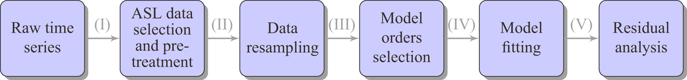
Figure 6. Diagrammatic flow of applying the ARMA model to boundary-layer turbulence.
There are two significant distinctions from traditional statistical practice in our procedure. First, the precondition of stationarity is required before employing the ARMA model. The traditional statistical modelling methods require only the removal of mean value by applying a moving average or a differential operator and the removal of periodic signals. Considering the physics of the ASL, we also need to ensure neutrality and filter large-scale synoptic signals. Second, the typical approach for ascertaining the model orders involves statistical criteria such as the Akaike or Bayesian information criterion (Choi Reference Choi2012). In contrast, within this study, we establish the model order based on the characteristic scale of the boundary layer, which again is restricted to ASL physics. This approach enhances the model's interpretability and endows the model with heightened physical significance.
Figure 7 shows an example of fitting the ARMA model. The half-hour raw fluctuating velocity series is presented in figure 7(a). Additionally, the reproduced coarse series is shown in figure 7(b). Using the ARMA model, we can regenerate the velocity series with almost the same velocity variance of raw data. Moreover, compared with the autocorrelation calculated from raw data, the autocorrelation generated by the ARMA(1,  $q$) model fits well, which is shown in figure 7(c). Figure 7(d) shows the corresponding second-order structure function, and the consistency between the result of the ARMA model and the proposed global expression indicates the validity of the approximate exponential function in the large-scale range. These results validate the applicability of using the ARMA(1, $q$) model to describe the boundary-layer streamwise velocity series.
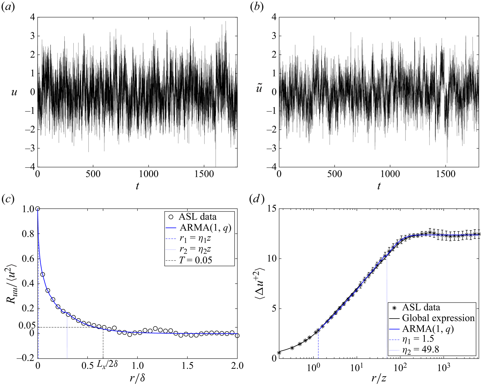
Figure 7. (a) Raw fluctuating velocity  $u$; (b) reproduced fluctuating velocity $\tilde u$; (c) comparison of autocorrelations of ASL data and ARMA model in normal-normal coordinates; and (d) comparison of the global expression, second-order structure functions of ASL data and ARMA model in log-normal coordinates, where $u_\tau =0.37$ m s $^{-1}$, ${Re}_\tau =3.78\times 10^6$ and $z^+=2.27\times 10^4$.
As discussed in § 2.1, we simplify the attached eddies with continuously varying sizes to a series of eddies whose sizes are approximated as a multiple of  $z$ up to $\delta$. The model parameters $\beta _i$ quantify these attached eddies’ effects on the current position's acceleration. Figure 8(a) shows that at all heights, as the distance $i\Delta x$ increases, the effect of corresponding attached eddies ( $\beta ^2_i$) decreases, indicating that the attached eddies with larger size contribute less to the fluctuating velocity. In addition, the model's memory depth is restricted to the dynamic range, where autocorrelation shows a logarithmic behaviour. Figure 8(b) shows that the self-similar random effect with a $-2$ power scaling of $\beta _i$ leads to a logarithmic autocorrelation, which is discussed in detail in Appendix B.

Figure 8. Fitted model parameters  $\beta _{i}$, $i=1,2,\ldots,q$, with ${Re}_\tau =3.78\times 10^6$.
Here, the ARMA(1,  $q$) model is used to model the dynamic range and to obtain the large-scale range's behaviour as a natural extension. To justify the large-scale behaviour, in figure 9, we show the premultiplied spectra, whose peak is used to distinguish large- and very-large-scale motions (Wang & Zheng Reference Wang and Zheng2016). Even though small scales are not resolved by the ARMA(1, $q$) model, its premultiplied spectra well captures that of the ASL data. Note that since the one-dimensional spectra at low wavenumber contain an aliasing effect, one needs to be careful when examining large-scale information from one-dimensional spectra. Improved approaches include examining two-dimensional spectra (Tong & Nguyen Reference Tong and Nguyen2015) and employing Fourier cutoff techniques (Ding et al. Reference Ding, Nguyen, Liu, Otte and Tong2018).

Figure 9. (a) Power spectra  $\varPhi _{uu}$ and (b) premultiplied spectra $k_x\varPhi _{uu}$ obtained from ASL data and ARMA(1, $q$) model, respectively. Here ${Re}_\tau =3.78\times 10^6$ and $z^+=7.55\times 10^5$.
3.3. Asymptotic global expression of the second-order structure function
Because the exact expression of the second-order structure function calculated from the ARMA(1,  $q$) model is complicated, for analytic simplicity, we derive a global asymptotic expression for the second-order structure function $\langle \Delta u^{+2} \rangle$ in § 2.3 (cf. (2.10), (2.11) and (2.16)), which is justified in figure 10(a). The uncertainty ranges of parameters $M_2$, $\xi _2$ and $\eta _1$ are discussed in Appendix C. Additionally, $\eta _2$ is calculated from (2.15b) with the optimized $\eta _1$. The parameters of inertial and dynamic ranges are close to the results of de Silva et al. (Reference de Silva, Marusic, Woodcock and Meneveau2015).

Figure 10. (a) Comparison of  $\langle \Delta u^{+2} \rangle$ obtained from ASL data and global asymptotic expression at ${Re}_\tau =3.78\times 10^6$. The intermediate scales of theoretical curves are as follows: Curve 1 – $\eta _1 = 1.06$, $\eta _2 = 27.71$; Curve 2 – $\eta _1 = 0.87$, $\eta _2 = 23.12$; Curve 3 – $\eta _1 = 0.73$, $\eta _2 = 15.42$. The black curves correspond to expressions for inertial and dynamic ranges presented by de Silva et al. (Reference de Silva, Marusic, Woodcock and Meneveau2015). (b) Comparison of $\eta _2$ obtained from ASL data and the expression (2.18) with $A_1/B_2=1.15$, $A_2/B_2=1/\xi _2=1.50$, $B_1/B_2=0.41$ and $B_1=0.80$.
According to (2.18),  $\eta _2/\eta _1$ is a power function of $z/\delta$, which we check in figure 10(b). This exponent is conventionally regarded to be $1$, corresponding to the empirical values of $B_1=1.25$ and $B_2=2.5$. However, in ASL data, $B_1$ often deviates from 1.25, and some researchers argue that $B_1$ may decrease with increasing $Re_\tau$ (Monkewitz Reference Monkewitz2022). In addition, $B_2$ depends on $\eta _1$ (cf. (2.11)), which is influenced by the ratio between the energy production and dissipation rate. So instead of restricting the values of $B_1$ and $B_2$ individually, we take the realistic values obtained from ASL data to test our expressions.
Furthermore, we undertake validation of the global expression through direct numerical simulation (DNS) and experimental results. Illustrated in figure 11(a), the triangle symbols correspond to the DNS data at  ${Re}_\tau \approx 5200$ obtained from Johns Hopkins turbulence database (Lee & Moser Reference Lee and Moser2015). Although the logarithmic slope $B_2$ of DNS data ranges from 1.46 to 1.78, smaller than the previously reported range of 2.16 to 2.5, the global expression matches the data well. The circle and square symbols in figure 11(a) correspond to the experiment results at ${Re}_\tau = 19\,000$, as detailed by Hutchins et al. (Reference Hutchins, Nickels, Marusic and Chong2009) and portrayed in figure 3(a) of de Silva et al. (Reference de Silva, Marusic, Woodcock and Meneveau2015). Combining these results from experiment, DNS and ASL data, we conclude that the proposed global expression for the second-order structure function is applicable across friction Reynolds numbers from $O(10^4)$ to $O(10^6)$. Since $B_2$ varies significantly with $z^+$ in DNS data, it is more appropriate to check (2.15b) rather than (2.18). The relationship between $\eta _2$ and $\eta _1$ obtained by asymptotic matching conforms well to the data, as shown in figure 11(b).
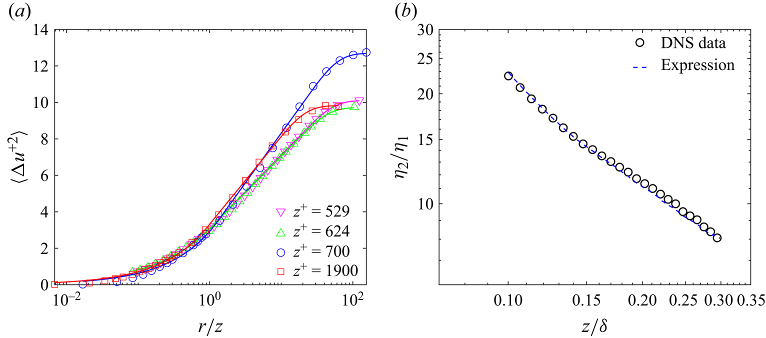
Figure 11. (a) Comparison of  $\langle \Delta u^{+2} \rangle$ obtained from DNS and experiment data and global asymptotic expression. Here, $z^+$ locates in the logarithmic region. The triangle symbols correspond to the DNS data at ${Re}_\tau \approx 5200$ (Lee & Moser Reference Lee and Moser2015), and the circle and square symbols correspond to the experiment data ${Re}_\tau = 19\,000$ (Hutchins et al. Reference Hutchins, Nickels, Marusic and Chong2009; de Silva et al. Reference de Silva, Marusic, Woodcock and Meneveau2015). (b) Comparison of $\eta _2$ obtained from DNS data and the expression (2.15b) with $A_1=1.72$ and $B_1=1.50$.
Introducing the two matching scales  $\eta _1$ and $\eta _2$ makes a more lucid examination of behaviours across distinct scale ranges feasible. Within the transport equation for the second-order structure function, the shear production term $\langle \Delta u\Delta w \rangle \,\mathrm {d} U/\mathrm {d} z$ injects energy into the shear boundary layers. So we explore the scaling behaviour of $\langle u_1w_2+u_2w_1 \rangle$. Figure 12(a) shows that the energy flux remains relatively constant within the inertial range (scales less than $\eta _1 z$). Additionally, in the dynamic range, $\langle u_1w_2+u_2w_1 \rangle$ follows a $-1$ power law that leads to the logarithmic expression for the structure functions (Xie et al. Reference Xie, de Silva, Baidya, Yang and Hu2021). Conversely, scales exceeding $\eta _2 z$ exhibit negligible production. So $\eta _2 z$ is an approximate indicator of the energy injection scale in boundary layers. With negligible energy flux, the autocorrelation in the active range decays exponentially.

Figure 12. Behaviour of covariance of streamwise velocity  $u$ and vertical velocity $w$ in the (a) dynamic range and (b) large-scale range.
One main result of the present study is obtaining the expression of the second-order structure function in the large-scale range, which is beyond previous works on the inertial and dynamic ranges (Davidson et al. Reference Davidson, Nickels and Krogstad2006b; Davidson & Krogstad Reference Davidson and Krogstad2014; de Silva et al. Reference de Silva, Marusic, Woodcock and Meneveau2015). In our extended expression, the upper bound of the dynamic range scales as  $\eta _2$. Thus, with scale normalized by $\eta _2 z$, collapse of data of different ${Re}_\tau$ in figure 13(a) justifies this characteristic scale. In the large-scale range, the exponential expression of the second-order structure functions obtained from the ARMA(1, $q$) model is justified in figure 13(b).

Figure 13. (a) Dynamic and large-scale ranges of second-order structure function with new scale  $\eta _2 z$ at different high friction Reynolds numbers ${Re}_\tau$. (b) Exponential scaling of the second-order structure function for scales larger than $\eta _2 z$.
3.4. The characteristic length scale
The asymptotic global expression for the second-order structure function provides a theoretical expression for characteristic length scales  $L_x$ identified by a threshold of autocorrelation. The well-fitting result of the global expression implies the validity of (2.22). There are three independent parameters in (2.22): $\eta _1$, $A_1/B_2$ and $B_1/B_2$. The empirical scale $\eta _1$ and already defined constants $A_1/B_2$ and $B_1/B_2$ characterize the variation of $L_x$. As shown in figure 14(a), the previous results of $L_x$ are summarized by Liu et al. (Reference Liu, Wang and Zheng2017) with an approximate logarithmic expression. However, other studies found anomalous behaviour of $L_x$ (Önder & Meyers Reference Önder and Meyers2018), suggesting that $L_x$ may be variant under different flow conditions. Our double-log expression (2.22) with turning parameters well captures all data, implying it as a robust relation.

Figure 14. (a) Characteristic length scales summarized by Liu et al. (Reference Liu, Wang and Zheng2017) and the data comes from Lee & Sung (Reference Lee and Sung2011), Volino, Schultz & Flack (Reference Volino, Schultz and Flack2007), Tutkun et al. (Reference Tutkun, George, Delville, Stanislas, Johansson, Foucaut and Coudert2009), Hutchins & Marusic (Reference Hutchins and Marusic2007), Hutchins et al. (Reference Hutchins, Chauhan, Marusic, Monty and Klewicki2012), Liu et al. (Reference Liu, Wang and Zheng2017) and Önder & Meyers (Reference Önder and Meyers2018). Equation (2.22) provides the prediction of parameters  $A_1/B_2$ and $B_1/B_2$. (b) Some ASL data that deviate from the $L_x$ summarized by Liu et al. (Reference Liu, Wang and Zheng2017) can also be characterized by (2.22). The height-averaged ratio of energy production and dissipation rate $P/\varepsilon$ for the time intervals corresponding to the circle, triangle and square symbols are 1.84, 1.47 and 1.37, respectively.
To further justify (2.22), in figure 14(b), we select three sets of ASL data with abnormal  $L_x$. Equation (2.22) also describe these behaviours with parameters $A_1/B_2$ and $B_1/B_2$ obtained from the streamwise fluctuating velocity variance and second-order structure function of the corresponding data sets. Note that in (2.22), in addition to $A_1/B_2$ and $B_1/B_2$, there is another parameter $\eta _1$ that needs to be determined, which is of order unity. In figure 14(a), $\eta _1$ is assumed to be 1 while it is taken as its average value at different heights in figure 14(b). The well-fitting results show that (2.22) is a good candidate to explain the variation of $L_x$.
Here our primary parameter of interest is  $B_1/B_2$, which although has an accepted value of $0.5$, deviates in different flows. As can be observed from the expression for $L_x$ in the large-scale range (cf. (2.22)), the extent to which $B_1/B_2$ deviates from 0.5 leads mainly to the growth rate of $L_x/\delta$ with $z/\delta$. Figure 14(b) shows that, usually, a smaller value of $B_1/B_2$ corresponds to a larger set of $L_x/\delta$. In uncontrollable ASL measurements, flow parameters that deviate from the standard zero-pressure-gradient boundary layer are not rare, e.g. production and dissipation are not locally balanced, and the height dependence of turbulent kinetic energy can vary (cf. (2.17)). The unbalanced energy production and dissipation affects the intermediate scale $\eta _1$ between inertial and dynamic ranges (Zhang et al. Reference Zhang, Xie and Zheng2022), thus impacting the value of $L_x$.
With the global expression, we can estimate the integral length scale  $\mathcal {L}$ approximately. For ASL data, because errors at large scales have a significant impact on the calculation of $\mathcal {L}$, we integrate the dimensionless autocorrelation up to the first 0.01 crossing scale, similar to the approach adopted by O'Neill et al. (Reference O'Neill, Nicolaides, Honnery and Soria2004) and Tritton (Reference Tritton2012). As shown in figure 15, (2.29a) characterizes the variation of $\mathcal {L}$ well. Since $f_1$ is sensitive to the value of $\mu$, see figure 4, we determine the value of $\mu$ from ASL data rather than using empirical values and the small-scale power exponent is set as $\xi _2=2/3$. Additionally, as discussed in § 2.4.3, (2.29) indicates that $\mathcal {L}$ locates in the dynamic range, suggesting that $\mathcal {L}$ is a characteristic scale of the attached eddies in the logarithmic region.

Figure 15. Comparison of integral length scale  $\mathcal {L}$ and approximate expression (2.29a). The autocorrelation is integrated up to the first 0.01 crossing. The parameter $\mu$ in $f_1$ is obtained from ASL data and $\xi _2=2/3$.
4. Summary and discussion
To model the streamwise velocity and explore the autocorrelation in boundary-layer turbulence, we apply the ARMA model to the dynamic and large-scale ranges of the second-order structure function. Consistent with the knowledge of boundary-layer turbulence and AEM, the memory depth  $q$ in the ARMA(1, $q$) model is determined by the lower and upper end of the dynamic range normalized by $z$,
$z$,  $\eta _1$ and $\eta _2$, respectively. The MA random effect in the ARMA(1, $q$) model dominates the behaviour of the dynamic range. A logarithmic second-order structure function is obtained when the randomness is self-similar, whose strength is captured by a power function with exponent $-2$. Additionally, we may regard the ARMA model as a stochastic AEM by the analogous linear additive random effects.
The ARMA model provides a natural extension of the second-order structure-function expression to the large-scale range (scales larger than  $\eta _2 z$), where the autocorrelation of streamwise velocity decays exponentially. We match the expression for the dynamic range and an exponential expression at $\eta _2$ to the second-order derivative to obtain an approximate global expression for the second-order structure function $\langle \Delta u^{+2} \rangle$ (cf. (2.10), (2.11) and (2.16)). In the global expression, the large- and small-scale coefficients are connected by asymptotically matching at characteristic scales $\eta _1$ and $\eta _2$. For example, for inertial and dynamic ranges, only three of the five coefficients ( $M_2$, $\xi _2$, $\eta _1$, $A_2$ and $B_2$) of the second-order structure-function expression are free and the global expression is determined after additionally determining the streamwise turbulence intensity $\langle u^{+2} \rangle$. This global expression is checked to be robust by well capturing the measured ASL data with non-canonical conditions and is applicable across friction Reynolds number from $O(10^4)$ to $O(10^6)$. Despite errors in autocorrelation and second-order structure function at large scales, the proposed expression yields an accurate calculation of the maximum energy injection scale $\eta _2$ and provides a method for determining the characteristic scale of the dynamic range from the streamwise turbulent intensity. These characteristic scales are relevant to other length scales in boundary-layer turbulence, as studied by Gustenyov et al. (Reference Gustenyov, Egerer, Hultmark, Smits and Bailey2023). For example, in the near-wall region, the energetic scale approximates the upper bound of the inertial range, which is close to the scale $\eta _1 z$. Additionally, the interface wavelength quantifying the average distance between two near turbulent regions corresponds to the peak of premultiplied spectra, which is consistent with $\eta _2 z$, indicating that in ASL, the large-scale range may be affected by the non-turbulent external atmospheric environment.
Based on the expression of  $\langle \Delta u^{+2} \rangle$, the expression for the streamwise characteristic scale $L_x$ is obtained. When the threshold of the autocorrelation locates in the large-scale range, the ARMA model implies that the characteristic scale has a double-log dependence on the distance to the wall, which resembles the traditional log-dependence in the parameter regimes with local energy production–dissipation balance and $B_1/B_2\approx 0.4$. In addition, our expression is also valid for non-standard situations, which is justified using ASL data with the Townsend–Perry constant and the logarithmic slope of $\langle \Delta u^{+2} \rangle$ deviating from their standard values. Thus, the robustness of this expression implies that the ARMA model captures certain underlying mechanisms in boundary-layer turbulence.
The exponential form of  $\langle \Delta u^{+2} \rangle$ based on the ARMA model, which links the dynamic range and the infinitely large scale, can be used to explain the previously proposed relation that the logarithmic slope of $\langle \Delta u^{+2} \rangle$ is twice that of the streamwise turbulent intensity $\langle u^{+2} \rangle$ in the logarithmic region. For instance, Davidson et al. (Reference Davidson, Nickels and Krogstad2006b) matched the dynamic range with the expression for streamwise turbulence intensity directly to obtain
 $$\begin{gather} \langle \Delta u^{+2} \rangle \left(r\right)= A_2+B_2\ln \left(r/z\right), \quad z< r\ll \delta, \end{gather}$$
 $$\begin{gather}\langle \Delta u^{+2} \rangle =2\langle u^{+2} \rangle = 2 \left[ A_1+B_1\ln \left(\delta/z\right)\right], \quad r\sim\delta, \end{gather}$$
where the coefficients  $B_2$ in (4.1a) and $2B_1$ in (4.1b) are equal. This matching procedure assumes that the logarithmic behaviour of $\langle \Delta u^{+2} \rangle$ lasts to the scale of $r = O(\delta )$ and that the the autocorrelation at $r = O(\delta )$ is negligible so $\langle \Delta u^{+2} \rangle \approx 2\langle u^{+2} \rangle$. However, without an expression for the range $r \geq O(\delta )$, the validity of the above assumptions is not solid. Additionally, based on the empirical value of $L_x$ larger than $\delta$, we know that when $r=\delta$, the second-order structure function is at least smaller than $1.9 \langle u^{+2} \rangle$. By proposing an expression of the large-scale range of $\langle \Delta u^{+2} \rangle$ using the ARMA model, we find when $\eta _2/\eta _1$ approximates $\delta /z$, their procedure is valid (cf. (2.19)), while for other cases, the double relation between $B_1$ and $B_2$ is modified.
Also, we obtained a lower bound of  $\langle u^{+2} \rangle$ in the logarithmic region, which is consistent with the existing numerical and experimental results (Hutchins et al. Reference Hutchins, Chauhan, Marusic, Monty and Klewicki2012; Wang & Zheng Reference Wang and Zheng2016). A dependence of this lower bound on the ratio of energy production to dissipation is proposed but remains to be checked. The global expression also yields an estimation of the integral length scale $\mathcal {L}$ (cf. (2.29)), which agrees well with the ASL data. Additionally, we conclude that in the logarithmic region of boundary-layer turbulence, $\mathcal {L}$ locates in the dynamic range of structure function and is a characteristic scale of attached eddies. A statistical study with more ASL data may be able to better validate (2.29a). In future studies, the same analytical procedure can be applied to the spanwise and wall-normal velocity series to explore the variation pattern of the corresponding characteristic length scales. Additionally, we can apply the ARMA( $\kern 0.06em p$, $q$) model with $p>1$. For the multivariate case, the vector ARMA model may be used to detect spatial information such as the inclination angle of coherent structures (Li et al. Reference Li, Hutchins, Zheng, Marusic and Baars2022). For convective ASL, a new range emerges due to the buoyancy effect, as delineated by the multi-point Monin–Obukhov similarity theory (Tong & Nguyen Reference Tong and Nguyen2015), and the combination of ARMA model and tempered fractional derivative (Samiee, Akhavan-Safaei & Zayernouri Reference Samiee, Akhavan-Safaei and Zayernouri2022) has the potential to capture the multi-scaling behaviour of structure functions.
Data errors and some assumptions limit the validation of present results. (i) The wall shear stress is not directly measured in QLOA and therefore the friction velocity  $u_\tau$ is approximated by the shear Reynolds stress. (ii) The orders of the ARMA model are all integers. Inevitably, errors are caused by extracting new series and implementing discrete models on continuous flow motion. (iii) Though we propose an approximate expression for $\langle \Delta u^{+2} \rangle$, its accuracy remains to be checked at large scales due to the error arising from Taylor's frozen hypothesis (He, Jin & Yang Reference He, Jin and Yang2017). This hypothesis is the only valid method for the current data to convert temporal data to the spatial domain, which is a common practice for ASL data analysis. For spatial data, the reformulation of the ARMA model is straightforward by replacing temporal separations with spatial separations, and it has the potential to capture more accurate physical information by avoiding the error brought about by the application of Taylor's frozen hypothesis.
Acknowledgements
We acknowledge valuable discussion with Yating Wan and open access direct numerical simulation data from Johns Hopkins turbulence databases.
Funding
F.-C.Z. and J.-H.X. gratefully acknowledge the financial support from the National Natural Science Foundation of China under Grant Nos. 92052102 and 12272006, and Joint Laboratory of Marine Hydrodynamics and Ocean Engineering, Laoshan Laboratory under Grant No. 2022QNLM010201. S.X.C. gratefully acknowledges financial support from the National Natural Science Foundation of China Grant No. 12292983. X.Z. gratefully acknowledges financial support from the National Natural Science Foundation of China Grant No. 92052202.
Declaration of interests
The authors report no conflict of interest.
Appendix A. Theoretical properties of the ARMA model
For an ARMA( $\kern 0.06em p$, $q$) model expressed as
 \begin{equation} u_t=\sum_{i=1}^{p}\alpha_i u_{t-i\Delta t}+\sum_{j=1}^{q}\beta_j\epsilon_{t-j\Delta t}+\epsilon_t, \end{equation}
or
 \begin{equation} A(\mathcal{B})u_t=B(\mathcal{B})\epsilon_t, \end{equation}
where  $\mathcal {B}$ is the time lag operators with lag $\Delta t$, i.e. $\mathcal {B}^i u_t=u_{t-i\Delta t}$, and $A$ and $B$ are linear operators defined as $A(\mathcal {B})=1-\sum _{i=1}^{p}\alpha _i\mathcal {B}^i$ and $B(\mathcal {B})=1+\sum _{j=1}^{q}\beta _j\mathcal {B}^j$, respectively. The time step $\Delta t$ could be chosen as the time interval corresponding to the measurement frequency of the time series or an artificially selected time step. The model equation (A1) or (A2) constrains the velocity at the moment $t$ to be influenced up to the velocities of the previous $p$ time steps (AR part) and the random noises of the previous $q$ time steps (MA part).
If the ARMA model can be applied to the time series, some restrictions must be satisfied. For example, if  $\{u_t\}$ is a causal function of $\{\epsilon _t\}$, there exists
 \begin{equation} u_t=\psi_0+\psi_1 \epsilon_{t-\Delta t}+\psi_2 \epsilon_{t-2\Delta t}+\cdots=\varPsi(\mathcal{B})\epsilon_t, \end{equation}
where the parameters should satisfy  $\sum _{i=0}^\infty |\psi _i|<\infty$ or $\varPsi (z)\neq 0$ for $|z|\leq 1$. Additionally, the series { $u_t$} should be an invertible function of { $\epsilon _t$}, i.e.
 \begin{equation} \epsilon_t=\vartheta_0+\vartheta_1 u_{t-\Delta t}+\vartheta_2 u_{t-2\Delta t}+\cdots = \varTheta(\mathcal{B})u_t, \end{equation}
where the parameters should satisfy  $\sum _{i=0}^\infty |\vartheta _i|<\infty$ or $\varTheta (z)\neq 0$ for $|z|\leq 1$. Also, the series is stationary if and only if $\varPsi (z)\neq 0$ for $|z|=1$.
A.1. Autocorrelation
Since the model equation is linear, some basic properties of the ARMA model can be expressed explicitly, such as the autocorrelation
 \begin{equation} R_{uu}(k\Delta t)=\langle u_t u_{t-k\Delta t} \rangle , \end{equation}
where  $k$ is the number of time steps and the angular brackets denote the time average over $t$. Since (A1) is a linear equation and the white noise $\epsilon _t$ is temporal independent, the autocorrelation of $u_t$ can be calculated directly as
 \begin{equation} R_{uu}(k\Delta t)= \sigma_\epsilon^2\sum_{i=0}^{\infty}\varphi_{i}\varphi_{i+k}, \end{equation}
where  $\varphi _0=\beta _0=1, \varphi _k=H(q-k)\beta _k+\sum _{i=1}^{min\{k,p\}}\alpha _i\varphi _{k-i}$. This is a convenient calculation method but without an explicit expression. An alternative method to obtain autocorrelation is to exploit the independence of white noise:
 \begin{align} R_{uu}(k\Delta
t)&=\langle u_t u_{t-k\Delta t} \rangle ,\nonumber\\
&=\left\langle \begin{pmatrix}\displaystyle\sum_{i=1}^{p}\alpha_i u_{t-i\Delta
t}+\sum_{j=0}^{q}\beta_j\epsilon_{t-j\Delta t} \end{pmatrix}
\begin{pmatrix}\displaystyle\sum_{i=1}^{p}\alpha_i u_{t-k\Delta t-i\Delta
t}+\sum_{j=0}^{q}\beta_j\epsilon_{t-k\Delta t-j\Delta t}
\end{pmatrix} \right\rangle ,
\end{align}
\begin{align} R_{uu}(k\Delta
t)&=\langle u_t u_{t-k\Delta t} \rangle ,\nonumber\\
&=\left\langle \begin{pmatrix}\displaystyle\sum_{i=1}^{p}\alpha_i u_{t-i\Delta
t}+\sum_{j=0}^{q}\beta_j\epsilon_{t-j\Delta t} \end{pmatrix}
\begin{pmatrix}\displaystyle\sum_{i=1}^{p}\alpha_i u_{t-k\Delta t-i\Delta
t}+\sum_{j=0}^{q}\beta_j\epsilon_{t-k\Delta t-j\Delta t}
\end{pmatrix} \right\rangle ,
\end{align}
where  $\langle {\sum }_{i=1}^{p}\alpha _i u_{t-i\Delta t}{\sum }_{i=1}^{p}\alpha _i u_{t-k\Delta t-i\Delta t} \rangle$ can easily be obtained since $\langle u_{t-i\Delta t}u_{t-j\Delta t} \rangle =R_{uu}(|i-j|\Delta t)$, and $\langle {\sum }_{j=0}^{q}\beta _j\epsilon _{t-j\Delta t}{\sum }_{j=0}^{q}\beta _j\epsilon _{t-k\Delta t-j\Delta t} \rangle$ can be calculated since $\langle \epsilon _{t-i\Delta t}\epsilon _{t-j\Delta t} \rangle =\delta _{ij}\sigma ^2_\epsilon$. For the other two terms, if $p\geq q$, the calculations are as follows:
 \begin{align} &\left\langle \sum_{i=1}^{p}\alpha_i u_{t-i\Delta t}\sum_{j=0}^{q}\beta_j \epsilon_{t-j\Delta t} \right\rangle \nonumber\\ &\quad= \langle {\alpha_1 u_{t-\Delta t}( \beta_1\epsilon_{t-\Delta t}+\beta_2\epsilon_{t-2\Delta t}+\cdots +\beta_q\epsilon_{t-q\Delta t} )}\nonumber\\ &\qquad +{\alpha_2 u_{t-2\Delta t}( \beta_2\epsilon_{t-2\Delta t}+\beta_3\epsilon_{t-3\Delta t}+\cdots +\beta_q\epsilon_{t-q\Delta t} )}+\cdots\nonumber\\ &\qquad +{\alpha_{q-1} u_{t-(q-1)\Delta t}( \beta_{q-1}\epsilon_{t-(q-1)\Delta t}+\beta_q\epsilon_{t-q\Delta t})}+{\alpha_{q} u_{t-q\Delta t}\beta_q\epsilon_{t-q\Delta t}}\rangle\nonumber\\ &\quad =\sum_{i=1}^{q}\sum_{j=i}^{q}\alpha_i \beta_j \varphi_{j-i}\sigma_\epsilon^2. \end{align}
A similar approach is taken for the case  $p< q$. Then (A7) can be simplified as
 \begin{equation} R_{uu}(k\Delta t)=\left\{ \begin{array}{ll} \displaystyle\sum_{i=1}^{p}\alpha_i^2R_{uu}(0)+2\sum_{i=1}^{p-1}\sum_{j=i+1}^{p}\alpha_i \alpha_j R_{uu}\left((\,j-i)\Delta t\right) & \\ \qquad +\displaystyle\sum_{i=0}^{q}\beta_i^2\sigma^2_\epsilon+2\sum_{i=1}^{min\{p,q\}}\sum_{j=i}^{q}\alpha_i \beta_j \varphi_{j-i}\sigma_\epsilon^2, & k=0,\\ \displaystyle\sum_{i=1}^{p}\alpha_i R_{uu}\left(|k-i|\Delta t\right)+H(q-k)\sum_{i=k}^{q}\beta_i \beta_{i-k} \sigma_\epsilon^2 & \\ \qquad +\, H(q-1-k)\displaystyle\sum_{i=1}^{min\{q-k,p\}}\sum_{j=k+i}^{q}\alpha_i \beta_j \varphi_{j-i-k}\sigma_\epsilon^2, & k\geq 1, \end{array} \right. \end{equation}
where  $H$ is a Heaviside function. Given the parameters $\alpha$, $\beta$ and $\sigma _{\epsilon} ^2$, the linear equations $R_{uu}(0), R_{uu}(\Delta t),\ldots,R_{uu}(\,p\Delta t)$ can be solved according to (A9) and the autocorrelation can be obtained.
Regardless of the method of calculation used, once the model parameters  $\alpha$, $\beta$ and $\sigma _{\epsilon} ^2$ are fitted, the autocorrelation $R_{uu}$ can be obtained explicitly. By comparing the autocorrelation calculated from the model parameters with the autocorrelation of data, it is intuitive to determine the applicability of the ARMA model.
Note that the Heaviside step function in (A9) leads to distinctive ranges of  $R_{uu}$. In particular, when $k\leq \max \{p, q\}$, the behaviour of autocorrelation can only be approximately derived under some assumptions, an example of which is given in Appendix B. When $k > \max \{p, q\}$, (A9) becomes
 \begin{equation} R_{uu}(k\Delta t)=\displaystyle\sum_{i=1}^{p}\alpha_i R_{uu}\left((k-i)\Delta t\right)\!. \end{equation}
Namely, when the considered data are beyond the model's memory depth  $(\max \{p\Delta t, q\Delta t\})$, the autocorrelation is only related to its history. Equation (A10) is a linear homogeneous recurrence relation whose characteristic equation is
 \begin{equation} \lambda^{p}-\alpha_1\lambda^{p-1}-\alpha_2\lambda^{p-2}-\cdots -\alpha_{p}=0. \end{equation}
If (A11) has  $p$ unequal roots $\lambda _1, \lambda _2,\ldots,\lambda _{p}$, its solution has the following form:
 \begin{equation} \lambda=c_1 \lambda_1^n +c_2 \lambda_2^n+\cdots+c_{p} \lambda_{p}^n, \end{equation}
where  $c_1, c_2,\ldots,c_{p}$ are constants. Then $R_{uu}$ has a general expression:
 \begin{equation} R_{uu}(k\Delta t)=\displaystyle\sum_{i=1}^{p}c_i \lambda_i^{k\Delta t} =\displaystyle\sum_{i=1}^{p}c_i \exp\left(k\Delta t\ln \lambda_i\right). \end{equation}
Or if (A11) has  $t$ unequal roots $\lambda _1, \lambda _2,\ldots,\lambda _{t}$, and the multiple numbers of roots are $m_1, m_2,\ldots,m_{t}$ ( $m_i\geq 1$ and $\sum _{i=1}^{t}m_i=p$), then the solution has the following form:
 \begin{align} \lambda&=(c_{1,0}n^0+c_{1,1}n^1+\cdots +c_{1,m_1-1}n^{m_1-1})\lambda_1^n+\cdots\nonumber\\ &\quad +(c_{t,0}n^0+c_{t,1}n^1+\cdots +c_{t,m_t-1}n^{m_t-1})\lambda_t^n, \end{align}
where  $c_{i,j} (i=1,\ldots,t,\,j=0,\ldots,m_i-1)$ are constants. In this case, $R_{uu}$ is still composed of exponential functions.
The above analysis implies that, beyond the model's memory depth, a set of exponential functions comprise the autocorrelation, which is mainly controlled by the parameters of the AR part and not affected explicitly by the MA part.
A.2. Power spectral density
After obtaining the model parameters, we can calculate the power spectral density of the ARMA model:
 \begin{equation} \varPhi_{uu}(k_x)=\frac{\sigma_\epsilon^2}{2{\rm \pi}} \left|\frac{B(\mathrm{i} k_x)}{A(\mathrm{i} k_x)} \right|^2, \end{equation}
where  $A$ and $B$ are functions defined in (A2), and $k_x$ is the wavenumber and the corresponding wavelength ${\unicode{x2113}}=2{\rm \pi} /k_x$. Because the power spectra and the autocorrelation are Fourier pairs, they provide the same statistical information of time series with different forms. In addition, the premultiplied power spectra $k_x\varPhi _{uu}$ illustrates the contribution of various wavenumber to the total spectra and identifies the wavenumber with the peak spectral density, which is commonly used to reveal large- and very-large-scale motions in boundary-layer turbulence. This work can also indicate how well the model's large-scale exponential behaviour approximates the data by comparing the premultiplied spectra of the ARMA model and the measured ASL data. Details and more information about the ARMA model presented here can be found from Shumway et al. (Reference Shumway, Stoffer and Stoffer2000).
Appendix B. Logarithmic behaviour of the autocorrelation of the ARMA(1,  $q$) model

Multiplying both sides of the equation of the ARMA(1,  $q$) model (cf. (2.6)) by $u_{t+\tau }$ and taking the average, we get
 \begin{equation} R_{uu}(\tau)=\alpha R_{uu}(\tau+\Delta t)+\sum_{i=0}^{q}\beta_i\langle u_{t+\tau}\epsilon_{t-i\Delta t} \rangle . \end{equation}
The continuous form of (B1) can be expressed as
 \begin{equation} \frac{\mathrm{d} R_{uu}}{\mathrm{d} \tau}=-\tilde\alpha R_{uu} +\langle u_{t+\tau}\epsilon_{t} \rangle +\int_{1}^{q}\beta_s\langle u_{t+\tau}\epsilon_{t-s\Delta t} \rangle \,\mathrm{d} s, \end{equation}
where  $\beta _0=1$ is used and $\tilde \alpha =(1-\alpha )/\Delta t$ is a positive constant. Following the same process as calculating (A8), we obtain
 \begin{align} \langle
u_{t+\tau}\epsilon_{t-s\Delta t} \rangle &= \left\langle
\left(\alpha u_{t+\tau-\Delta
t}+\epsilon_{t+\tau}+\sum_{i=1}^q\beta_i\epsilon_{t+\tau-i\Delta
t}\right)\epsilon_{t-s\Delta t} \right\rangle \nonumber\\
&=\left\langle \left[\alpha \left(\alpha u_{t+\tau-2\Delta
t}+\epsilon_{t+\tau-\Delta
t}+\sum_{i=1}^q\beta_i\epsilon_{t+\tau-\Delta t-i\Delta
t}\right)+\epsilon_{t+\tau}\right.\right.\nonumber\\
&\left.\left.\quad
+\sum_{i=1}^q\beta_i\epsilon_{t+\tau-i\Delta
t}\right]\epsilon_{t-s\Delta t} \right\rangle
=\sigma_\epsilon^2\sum_{i=0}^Q\beta_i\alpha^{Q-i},
\end{align}
\begin{align} \langle
u_{t+\tau}\epsilon_{t-s\Delta t} \rangle &= \left\langle
\left(\alpha u_{t+\tau-\Delta
t}+\epsilon_{t+\tau}+\sum_{i=1}^q\beta_i\epsilon_{t+\tau-i\Delta
t}\right)\epsilon_{t-s\Delta t} \right\rangle \nonumber\\
&=\left\langle \left[\alpha \left(\alpha u_{t+\tau-2\Delta
t}+\epsilon_{t+\tau-\Delta
t}+\sum_{i=1}^q\beta_i\epsilon_{t+\tau-\Delta t-i\Delta
t}\right)+\epsilon_{t+\tau}\right.\right.\nonumber\\
&\left.\left.\quad
+\sum_{i=1}^q\beta_i\epsilon_{t+\tau-i\Delta
t}\right]\epsilon_{t-s\Delta t} \right\rangle
=\sigma_\epsilon^2\sum_{i=0}^Q\beta_i\alpha^{Q-i},
\end{align}
where  $Q=\min \{\tau /\Delta t+s, q\}$. Therefore, in a continuous limit,
 \begin{equation} \langle u_{t+\tau}\epsilon_{t-s\Delta t} \rangle =\sigma_\epsilon^2 \left( \alpha^{\tau/\Delta t+s}+ \int_{1}^{\tau/\Delta t+s} \beta_{s'} \alpha^{\tau/\Delta t+s-s'}\,\mathrm{d} s' \right) . \end{equation}
Assuming  $\beta '_s$ has a power-function form $\beta '_s\sim s'^{-\gamma }$ when $s'>1$, to the leading order, we obtain
 \begin{equation} \langle u_{t+\tau}\epsilon_{t-s\Delta t} \rangle \sim \int_{1}^{\tau/\Delta t+s} s'^{-\gamma}\alpha^{\tau/\Delta t+s-s'}\,\mathrm{d} s' \sim(\tau/\Delta t+s)^{-\gamma+1}. \end{equation}
 Since  $\langle u_{t+\tau }\epsilon _{t-s\Delta t} \rangle$ decreases as $s$ increases according to (B5) and $\beta _s$ also decays, the integrand in (B2) is the convolution of $\langle u_{t+\tau }\epsilon _{t} \rangle$ with the kernel function $\beta _s$ and it is therefore less than $\langle u_{t+\tau }\epsilon _{t} \rangle$. Thus, the solution of (B2) is dominated by
 \begin{equation} R_{uu}\sim \mathrm{e}^{-\tilde\alpha \tau} \left( \int_{\tau_0}^{\tau} \mathrm{e}^{\tilde\alpha s'} \langle u_{t+s'}\epsilon_{t} \rangle \,\mathrm{d} s' +R_{uu}(\tau_0) \right). \end{equation}
Substituting (B5) into the above approximation, we obtain
 \begin{equation} R_{uu}\sim \mathrm{e}^{-\tilde\alpha \tau} \int_{\tau_0}^{\tau} \mathrm{e}^{\tilde\alpha s'} (s'/\Delta t)^{-\gamma+1} \,\mathrm{d} s'. \end{equation}
Then, taking the leading terms in the Taylor expansion of exponential functions, we get
 \begin{equation} R_{uu}\sim \left( 1-O(\tilde\alpha) \right) \int_{\tau_0}^{\tau} \left( 1+O(\tilde\alpha) \right) (s'/\Delta t)^{-\gamma+1} \,\mathrm{d} s' \sim \int_{\tau_0}^{\tau} s'^{-\gamma+1} \,\mathrm{d} s'. \end{equation}
Particularly, when  $\gamma = 2$, we obtain
 \begin{equation} R_{uu}\sim \ln \tau. \end{equation}
Thus, the logarithmic behaviour of autocorrelation is a consequence of the power law of the MA coefficients  $\beta$, which justified the fitting result in figure 8(b).
Appendix C. Uncertainty in determining the global expression
As discussed in § 2.3, for a fixed height  $z$ with known $\langle u^{+2} \rangle$, the behaviour of the global expression for the second-order structure function is controlled by the transition scale $\eta _1$ and small-scale parameters $M_2$ and $\xi _2$. To compare the agreement between global expression and ASL data, we define an error
 \begin{equation} \mathcal{E}_0(\eta_1,M_2,\xi_2)=\int_{r_{min}}^{r_{max}} \frac{\left|\langle \Delta u^2 \rangle -G(\eta_1,M_2, \xi_2,r)\right|}{2\langle u^2 \rangle } \,\mathrm{d} \ln \left( \frac{r}{z} \right), \end{equation}
where  $G(\eta _1,M_2, \xi _2,r)$ is the global expression of second-order structure function with fixed $\eta _1$, $M_2$ and $\xi _2$, and $r_{min}$ and $r_{max}$ are the minimum and maximum scales of the structure function, respectively.
Here, we illustrate the uncertainty relating to the choice of  $\eta _1$ using
 \begin{equation} \mathcal{E}(\eta_1)= \min_{M_2,\xi_2}\mathcal{E}_0(\eta_1,M_2,\xi_2), \end{equation}
which is the minimum error for a fixed  $\eta _1$. Figure 16 shows the dependence of $\mathcal {E}$ on $\eta _1$. These cases correspond to those shown in figure 10(a), where the values of $\eta _1$ are determined from the minimum of $\mathcal {E}$. The uncertainty range of $\eta _1$ is quantified as the values with $\mathcal {E}$ ranging from $\mathcal {E}_{min}$ to $(1+5\,\%)\mathcal {E}_{min}$. Figure 16 and table 1 show a small uncertainty of $\eta _1$. The uncertainty ranges of other parameters are summarized in table 1.

Figure 16. Errors in the optimization of  $\eta _1$.
Table 1. Uncertainty ranges of  $M_2$, $\xi _2$ and $\eta _1$ in figure 10(a).