


1. Introduction
There is a long history of research examining the reflection of oblique shock waves generated from a wedge over a wall or symmetry plane in steady supersonic flows. In 1878, Mach (Reference Mach1878) was the first to observe two reflection configurations: regular reflection (RR) and Mach reflection (MR). The transition criteria between these two shock reflection types have been the subject of discussion for several decades. The two- and three-shock theories were developed by von Neumann (Reference von Neumann1943, Reference von Neumann1945) to describe RR and MR, respectively. The configurations given by these two theories are shown schematically in figures 1(a,b). In the case of RR, the incident shock wave (i) intersects with the reflecting surface (R) and produces a reflected shock wave (r). For MR, the incident and reflected shock waves are connected to the reflecting surface by another shock called the Mach-stem shock (m). These three shocks intersect at the triple point (T) and generate a slip line (s). The foot of the Mach stem is perpendicular to the reflecting surface. Based on these two theories, von Neumann (Reference von Neumann1943, Reference von Neumann1945) proposed the mechanical equilibrium criterion (now commonly referred to as the von Neumann criterion) and the detachment criterion. The former provides the minimum of the incident shock angle at which MR exists theoretically; the latter gives the maximum shock angle for the existence of RR. After further research, Mölder (Reference Mölder1979) noted that the von Neumann criterion has an applicable condition whereby the free-stream Mach number  $M_0$ must be greater than a certain Mach number $M_c$. The value of $M_c$ is related to the specific heat ratio $\gamma$ ( $M_c\approx 2.2$ while $\gamma =1.4$). For $M_0 > M_c$, there is a dual-solution domain in which both RR and MR are theoretically possible. This domain is identified in the $(M_0,\theta _i)$ plane in figure 1(c), where $\theta _i$ is the incident shock angle at the reflection point. In this plane, $\theta _{{max}}$, $\theta _D$, $\theta _N$ and $\theta _{{min}}$ represent the incident shock wave detachment criterion, von Neumann's detachment criterion, mechanical equilibrium criterion and Mach angle, respectively. RR can occur for $\theta _{{min}}<\theta _i<\theta _D$, and MR can occur for $\theta _N<\theta _i<\theta _{{max}}$; the dual-solution domain exists between $\theta _N$ and $\theta _D$. For MR, Chow & Chang (Reference Chow and Chang1974) suggested that the flow behind the reflected shock is supersonic ( $M_2 > 1$) for $\theta _i < \theta _S$, and subsonic ( $M_2 < 1$) for $\theta _i > \theta _S$, where $\theta _S$ corresponds to the incident shock angle at which $M_2 = 1$. While both RR and MR are stable in the dual-solution domain (Teshukov Reference Teshukov1989; Li & Ben-Dor Reference Li and Ben-Dor1996), they can transit each other with a disturbance whose threshold level exceeds a certain value (Ivanov, Kudryavtsev & Khotyanovskii Reference Ivanov, Kudryavtsev and Khotyanovskii2000; Kudryavtsev et al. Reference Kudryavtsev, Khotyanovsky, Ivanov and Vandromme2002). In RR-to-MR transition initiated by a small disturbance, a tiny Mach stem first appears and develops smoothly to the steady-state height. With the growth of the Mach stem, the triple point moves upstream along the incident shock wave.

Figure 1. Schematic of RR and MR along with domains for different reflection types in the  $(M_0,\theta _i)$ plane.
For flat-shock reflections, several studies have investigated the height of the Mach stem, the shape of the discontinuities (Mach stem, reflected shock and the slip line) and the time history of the RR-to-MR transition. Azevedo (Reference Azevedo1989) and Azevedo & Liu (Reference Azevedo and Liu1993) studied the Mach stem and developed a physical model to predict its height  ${H_m}$. In their research, the region bounded by the slip line and the reflecting surface was considered an effective one-dimensional converging nozzle. To describe the flow pattern, the quasi-one-dimensional isentropic relation was applied. The slip line was assumed to be linear before interacting with the leading expansion wave, which is where the sonic throat formed. Li & Ben-Dor (Reference Li and Ben-Dor1997) studied the interactions of the reflected shock with the expansion fan from the trailing edge of the wedge. They described a physical mechanism by which the centred expansion fan creates the sonic throat and determines the Mach-stem height. However, they ignored the influence of the reflected waves of transmitted expansion waves on the slip line. Mouton (Reference Mouton2007) suggested another model that considered only the geometrical features of the flow pattern while neglecting the curvature of discontinuities (Mach stem and slip line). Gao & Wu (Reference Gao and Wu2010) improved the model by further considering additional details, such as interactions between the transmitted expansion fan and the waves generated from the slip line.
In addition to the Mach-stem height, research on the shape of the Mach stem and other flow structures has attracted significant attention. Dewey & McMillin (Reference Dewey and McMillin1985a,Reference Dewey and McMillinb) studied experimentally the shapes of the incident, reflected and Mach-stem shocks for pseudo-steady reflections. They showed that the Mach stem was described well by a circular arc centred slightly below the reflecting surface. These experimental results were confirmed by Olim & Dewey (Reference Olim and Dewey1992) and Dewey & Barss (Reference Dewey and Barss1996). The shape of the Mach stem was also considered analytically by Li, Ben-Dor & Han (Reference Li, Ben-Dor and Han1994) for pseudo-steady reflections, and by Li & Ben-Dor (Reference Li and Ben-Dor1997) for steady flows from a geometric perspective. A second-order curve was used by Li & Ben-Dor (Reference Li and Ben-Dor1997) to model the Mach stem. By assuming that the angle between the slip line and the reflecting plane is sufficiently small, Tan, Ren & Wu (Reference Tan, Ren and Wu2006) described the flow immediately behind the Mach stem using the isentropic small-disturbance equation, and demonstrated that the Mach stem can be approximated by a circular arc of relatively small curvature. The shape of the reflected shock wave was analysed using the shock-expansion wave interaction method of Rosciszewski (Reference Rosciszewski1960) and Hasimoto (Reference Hasimoto1964), as well as by the approximate method of Li & Ben-Dor (Reference Li and Ben-Dor1995). Bai & Wu (Reference Bai and Wu2017) derived analytical expressions for the shape of the slip line and reflected shock wave.
In comparison to the structures of stable MRs, the time history of the RR-to-MR transition has rarely been considered. Mouton & Hornung (Reference Mouton and Hornung2007, Reference Mouton and Hornung2008) presented an approximate theory to predict the growth rate of the Mach-stem height. They assumed that the transition process contains a single but evolutionary MR. The evolutionary MR satisfies a steady-flow model when the reference frame is attached to the moving triple point. In their model, during the transition, the Mach stem and reflected shock wave were considered to be straight. Kudryavtsev et al. (Reference Kudryavtsev, Khotyanovsky, Ivanov and Vandromme2002) performed a series of numerical simulations to study the influence of disturbances on shock wave reflection transitions. Their results showed that a new shock interaction structure exists at the beginning of the transition. The mechanism of this new interaction structure in the time history of transitions was studied by Li, Gao & Wu (Reference Li, Gao and Wu2011); they developed an idealized unsteady model that divides the transition process into a multiple-interaction stage and a pure-MR stage to capture the time evolution of the Mach stem.
The above studies considered flat shock waves. With the enrichment of theoretical research on curved shock waves (Mölder Reference Mölder2015; Emanuel Reference Emanuel2019; Shi et al. Reference Shi, Han, Deiterding, Zhu and You2020), the reflection of curved shock waves has gradually attracted increasing attention. Mölder (Reference Mölder2015) proposed the curved shock theory (CST), which relates the flow gradients to the curvatures of shock waves. Emanuel (Reference Emanuel2019) and Shi et al. (Reference Shi, Han, Deiterding, Zhu and You2020) further developed the theory to higher dimensions and orders, respectively. Shi et al. (Reference Shi, Zhu, You and Zhu2021) derived the method of curved shock characteristics (MOCC) for calculating the supersonic flow field behind curved shock waves based on the CST. In 2017, the CST was applied to the reflection of a curved shock by Mölder (Reference Mölder2017). The curvatures of the reflected shock wave, Mach stem and slip line, as well as the pressure gradient around the reflection point, were derived. Based on this work, Shi (Reference Shi2021) proposed a geometric equation for the Mach stem and slip line in curved shock MRs (CMRs). According to this equation, the shape of the Mach stem should be determined by the position of the triple point.
The above-described research focused solely on the flow structure near the reflection point. However, for CMRs, the wave configuration of the triple point is not sufficient to reflect the properties of the whole flow field. For example, the position of the triple point, which determines the shape of the Mach stem, is unknown. To reveal the formation mechanisms of CMRs, the structure of the flow field and the time history of the RR-to-MR transition should be examined. Due to the non-uniform nature of the flow behind curved shock waves, traditional models for flat shock waves are no longer applicable. In this paper, an analytical model is established to predict the overall structure of CMRs using the CST and the MOCC. Details of the flow field are analysed using high-order flow parameters. In addition, the curved shock equations attached to the moving frame are derived to model the RR-to-MR transition process. The influence of the incident shock angle and isentropic waves (or Mach waves) on the moving velocity of the triple point is studied theoretically and numerically. Finally, the influence of the wall curvature on the transition time is evaluated. This work is of great importance to the design of hypersonic vehicles and supersonic engines.
2. Analytical model
First, we simulate numerically the reflection of a curved incident shock in the dual-solution domain to display the two possible reflection structures and their associated transition. Analytical models are then proposed to describe the structure and transition of curved shock reflections. Throughout this paper,  $\delta _w$, $D_w$, $H_0$ and $H_e$ are used to denote the initial deflection angle, wall curvature, and heights of the curved-wall inlet and outlet, respectively. The wall curvature is positive when the deflection angle increases while approaching the reflecting surface along the wall. This means that a positively curved wall is always concave towards the upstream flow.
Figure 2 provides the Mach number contours of the flow at a series of moments during the RR-to-MR transition in the dual-solution domain for  $M_0 = 5$, $\delta _w = 19^\circ$, $D_w H_0 = 0.12$ and $H_e/H_0=0.5$. The transition time $t$ has been normalized with the inlet height $H_0$ and free-stream sound speed $a_0$. The computational fluid dynamics (CFD) methods used throughout this paper and the density perturbation that is applied to induce transitions are introduced in Appendix A, which also shows a grid independence analysis to illustrate that the current grid set-up is sufficient to achieve the goals of this paper. When $t=0$, the disturbance has just reached the reflection point, and the flow field presents a structure of RRs, as shown in figure 2(a). The steepening of the incident shock wave in the disturbed region can be seen in the locally enlarged image of the reflection point. After a period of continuous disturbance, figure 2(b) shows that the Mach stem is induced locally at the reflection point to form a three-shock structure. At this point, the RR structure still exists macroscopically. As the Mach stem evolves, the shock reflected at the triple point intersects the reflected shock of the RR structure to form another triple point, as shown in figures 2(c–f). The second triple point moves along the reflected shock of the RR structure until disappearing. At the same time, a sonic throat begins to form under the slip line, as shown in figure 2(g). The triple point then moves upstream continuously and eventually stabilizes at the position shown in figure 2(h). These plots clearly indicate the curving of the incident shock wave and the non-uniformity of the post-shock flow field.

Figure 2. Instantaneous representations of the Mach contours during the RR-to-MR transition triggered by an upstream density disturbance for a concave incident shock ( $M_0 = 5$, $\delta _w = 19^\circ$, $D_w H_0=0.12$, $H_e/H_0 = 0.5$).
The current numerical method can be used to simulate the overall MR. However, due to the numerical viscosity, the slip line will display Kelvin–Helmholtz instability (Samtaney & Pullin Reference Samtaney and Pullin1996; Ivanov et al. Reference Ivanov, Ben-Dor, Elperin, Kudryavtsev and Khotyanovskii2002). The rolling of the slip line will produce parasitic waves that invalidate the CFD results (Gao & Wu Reference Gao and Wu2010). Therefore, it is necessary to model the flow field to ensure that the main flow structures are well captured. In the rest of this section, the analytical methods describing the flow configurations of CMRs and the RR-to-MR transition process are introduced.
2.1. Analytical model for stationary CMRs
Figure 3 depicts schematic illustrations of the two stable structures (RR and MR) displayed in figure 2. In the diagram, the incoming flow (0) passes a curved wall and generates a curved shock at the leading edge due to flow deflection. The curved incident shock (i) propagates downstream and intersects with the reflecting surface. It occasionally forms an RR structure and produces a reflected shock wave (r) from the rigid wall (figure 3a). In the case of MR (figure 3b), a Mach stem (m) appears between the reflection point and the reflecting surface. The Mach stem grows along the incident shock and remains stable at the triple point (T). Sometimes, if the incident shock angle is located in the dual-solution domain, an RR-to-MR transition can occur with an initial disturbance, as shown in figure 2. The time history of the Mach stem during the transition is helpful for revealing the formation mechanism of the CMR flow field. Before this, considering the non-uniformity of the flow behind curved shock waves, the steady-state MR first has to be studied to evaluate the influence of the non-uniform nature of the flow structure.

Figure 3. Schematic illustration of the stable curved shock reflection configurations: (a) regular reflections, and (b) Mach reflections.
As shown in figure 3(b), four discontinuities meet at the triple point: the incident shock, reflected shock, Mach stem and slip line (s). Downstream of the triple point, the reflected shock wave interferes with the expansion waves (e) generated by the trailing edge of the wall. The four discontinuities, along with the first expansion wave, divide the entire flow field into four regions. In general, regions (1), (2) and (4) are supersonic, and region (3) is subsonic. The subsonic flow pattern behind the Mach stem can be approximated as a one-dimensional flow and is similar to that through a de Laval nozzle. The height of the slip line decreases initially. This is followed by an increase in height, giving a minimum value at the throat (t), where the Mach number is equal to 1. Due to the complexity of the flow behind a curved shock wave, the four regions should be solved separately. The solution methods are introduced below.
2.1.1. Flow around the triple point
We use  $\rho$, $p$,
$p$,  $V$,
$V$,  $M$,
$M$,  $\delta$, $\theta$ and $\gamma$ to denote the density, pressure, velocity, Mach number, flow angle, shock angle and specific heat ratio of the gas, respectively. The following classical shock relations connect the downstream flow (subscript 1) to the upstream flow (subscript 0) of the incident shock:
 \begin{equation} \left. \begin{gathered} \frac{{{p_1}}}{{{p_0}}} = 1 + \frac{{2\gamma }}{{\gamma + 1}}\left( {M_0^2\sin^2{\theta _i} - 1} \right),\\ \frac{{{\rho _1}}}{{{\rho _0}}} = \frac{{\left( {\gamma + 1} \right)M_0^2\sin^2{\theta _i}}}{{\left( {\gamma - 1} \right)M_0^2\sin^2{\theta _i} + 2}},\\ \frac{{{V_1}}}{{{V_0}}} = \frac{{\cos {\theta _i}}}{{\cos ( {{\theta _i} - \delta } )}},\\ \tan ( {{\delta _1} - {\delta _0}} ) = 2\cot {\theta _i}\,\frac{{M_0^2\sin^2{\theta _i} - 1}}{{M_0^2\left( {\gamma + \cos ( {2{\theta _i}} )} \right) + 2}}. \end{gathered} \right\} \end{equation}
Equations (2.1) provide the flow parameters downstream of the shock. With the development of CST (Mölder Reference Mölder2015), the first-order post-shock parameters, which reveal more information about the flow near the shock, can be acquired with the following planar curved shock equations:
 \begin{equation} \left. \begin{gathered} {A_{0,i}}{P_0} + {B_{0,i}}{D_0} + {E_{0,i}}{\varGamma _0} = {A_{1,i}}{P_1} + {B_{1,i}}{D_1} + {C_{i}}{S_{a,i}},\\ A_{0,i}'{P_0} + B_{0,i}'{D_0} + E_{0,i}'{\varGamma _0} = A_{1,i}'{P_1} + B_{1,i}'{D_1} + C_{i}'{S_{a,i}},\\ A_{0,i}''{P_0} + B_{0,i}''{D_0} + E_{0,i}''{\varGamma _0} = A_{1,i}''{P_1} + B_{1,i}''{D_1} + E_{1,i}''{\varGamma _1} + C_{i}''{S_{a,i}}, \end{gathered} \right\} \end{equation}
where  $P$,
$P$,  $D$,
$D$,  $\varGamma$ and $S_a$ indicate the pressure gradient, streamline curvature, vorticity and shock curvature in the flow plane, respectively. The coefficients can be found in (Mölder Reference Mölder2015), and for planar flow, $S_b$ (i.e. the shock curvature in the flow-normal plane) is zero.
The shock relations and the three-shock theory provide the following relationships between the four discontinuities:
 \begin{equation} \left. \begin{gathered} \frac{{{p_2}}}{{{p_1}}} = 1 + \frac{{2\gamma }}{{\gamma + 1}}\left( {M_1^2\sin^2{\theta _r} - 1} \right),\\ \tan ( {{\delta _2} - {\delta _1}} ) = 2\cot {\theta _r}\,\frac{{M_1^2\sin^2{\theta _r} - 1}}{{M_1^2\left( {\gamma + \cos ( {2{\theta _r}} )} \right) + 2}},\\ \frac{{{p_3}}}{{{p_0}}} = 1 + \frac{{2\gamma }}{{\gamma + 1}}\left( {M_0^2\sin^2{\theta _m} - 1} \right),\\ \tan ( {{\delta _3} - {\delta _0}} ) = 2\cot {\theta _m}\,\frac{{M_0^2\sin^2{\theta _m} - 1}}{{M_0^2\left( {\gamma + \cos ( {2{\theta _m}} )} \right) + 2}},\\ {p_3} = {p_2},\\ {\delta _3} = {\delta _2}. \end{gathered} \right\} \end{equation}
The angle moving anticlockwise towards the  $x$ axis is regarded as positive. There are six unknowns in (2.3) for the six equations: $p_2$, $\delta _2$, $\theta _r$, $p_4$, $\delta _4$ and $\theta _m$. Thus the angles of the reflected shock, Mach stem and slip line, as well as the post-shock pressure at the triple point, can be solved from the incident shock angle and incoming conditions. Mölder (Reference Mölder2017) proposed the following equations based on the three-shock theory and CST to acquire the curvatures of the reflected shock, Mach stem and slip line as well as the pressure gradient at the triple point, where there are six unknowns, $P_2$, $D_2$, $S_{a,r}$, $P_4$, $D_4$ and $S_{a,m}$:
 \begin{equation} \left. \begin{gathered} {A_{1,r}}{P_1} + {B_{1,r}}{D_1} + {E_{1,r}}{\varGamma _1} = {A_{2,r}}{P_2} + {B_{2,r}}{D_2} + {C_{r}}{S_{a,r}},\\ A_{1,r}'{P_1} + B_{1,r}'{D_1} + E_{1,r}'{\varGamma _1} = A_{2,r}'{P_2} + B_{2,r}'{D_2} + C_{r}'{S_{a,r}},\\ {A_{0,m}}{P_0} + {B_{0,m}}{D_0} + {E_{0,m}}{\varGamma _0} = {A_{3,m}}{P_3} + {B_{3,m}}{D_3} + {C_{m}}{S_{a,m}},\\ A_{0,m}'{P_0} + B_{0,m}'{D_0} + E_{0,m}'{\varGamma _0} = A_{3,m}'{P_3} + B_{3,m}'{D_3} + C_{m}'{S_{a,m}},\\ M_3^2{P_3} = M_2^2{P_2},\\ {D_3} = {D_2}. \end{gathered} \right\} \end{equation}
2.1.2. Introduction of the MOCC and its application in regions (1) and (2)
The CST gives the shock curvature and flow divergence/convergence in terms of the pressure gradient, vorticity and streamline curvature. Once the incoming flow conditions have been determined, the post-shock parameters can be solved using the curved shock equations. However, these are tenable only near the shock. To calculate supersonic flow fields, Shi et al. (Reference Shi, Zhu, You and Zhu2021) derived the MOCC in (2.5) in the  $(s,l)$ plane, where $s$ denotes the streamline, and $l$ denotes the characteristic coordinates from the Euler equations:
 \begin{equation} \left. \begin{gathered} \frac{\mathrm{d}p}{\mathrm{d}l_\pm}-\rho V^2(P\cos\mu \mp D\sin\mu) = 0,\\ \frac{\mathrm{d}\delta}{\mathrm{d}l_\pm}-\frac{D\sin\mu \mp P\cos\mu}{\tan\mu} \pm j\,\frac{\sin\delta\sin\mu}{y} = 0,\\ \frac{\mathrm{d}p}{\mathrm{d}s}-\rho V^2P = 0,\\ \frac{\mathrm{d}\delta}{\mathrm{d}s}-D = 0,\\ \rho V\,\frac{\mathrm{d}V}{\mathrm{d}s}+\frac{\mathrm{d}p}{\mathrm{d}s} = 0,\\ \frac{\mathrm{d}p}{\mathrm{d}s}-\frac{\gamma p}{\rho}\,\frac{\mathrm{d}\rho}{\mathrm{d}s} = 0. \end{gathered} \right\} \end{equation}
 The equations for the left-running characteristic and streamline are solved in the  $(s,l+)$ coordinates for the external flow, whereas the equations for the right-running characteristic and streamline are evaluated in the $(s,l-)$ coordinates for the internal flow. There are six unknowns – $p$,
$p$,  $\delta$, $\rho$, $V$,
$V$,  $P$ and $D$ – in the six equations to describe a unit process that contains a streamline and characteristic line. Therefore, the MOCC extends the application area of CST from the region near the shock to the post-shock flow field.
Three unit algorithms (interior process, shock process and wall/parameter distribution process) are introduced by Shi et al. (Reference Shi, Zhu, You and Zhu2021). As shown in figure 3, the flow in region (1) is a typical internal flow with uniform inflow and known wall boundary conditions that can be solved using the interior, shock and wall processes. The flow pattern in region (3) is considered as a one-dimensional flow. Thus the following equations establish the relationship between the pressure and height of the slip line (where  $\bar {M}_m$ and $\bar {p}_m$ are the average Mach number and pressure just behind the Mach stem) as
 \begin{gather} \frac{y}{\bar{H}_m} = \frac{\bar{M}_m}{M}\left\{\frac{1+\left[(\gamma-1)/2\right]M^2}{1+\left[(\gamma-1)/2\right]\bar{M}_m^2}\right\}^{(\gamma+1)/2(\gamma-1)}, \end{gather}
 \begin{gather}\frac{p}{\bar{p}_m} = \left\{\frac{1+\left[(\gamma-1)/2\right]M^2}{1+\left[(\gamma-1)/2\right]\bar{M}_m^2}\right\}^{1/(\gamma-1)}. \end{gather}
Therefore, the flow over the slip line (region (2)) can be regarded as a non-uniform external flow with a known pressure distribution.
2.1.3. Expansion fan and its interactions with the reflected shock
To prevent choking in internal contraction flows, the wall is set to turn at a certain height to stabilize the flow field. Hence there are always interactions between the expansion waves generated by the sharp corner and the reflected shock. For flat-shock MRs, the flow behind the incident shock wave is uniform, and region (4) is a Prandtl–Meyer fan. However, for curved shock reflections, the flow in front of the expansion fan is no longer uniform. Therefore, expansion waves should disperse into segments for the calculations, as shown in figure 4. Taking points 1 and 3 along the direction of the expansion wave as an example, the relationship between the two points is
 \begin{gather} \frac{\mathrm{d}\delta}{\mathrm{d}l}-\frac{\sin\bar{\mu}}{\gamma\bar{p}}\,\frac{\mathrm{d}p}{\mathrm{d}l} = j\,\frac{\sin\bar{\delta}\sin\bar{\mu}}{\bar{y}}, \end{gather}
 \begin{gather}y_3 = y_1+(x_3-x_1)\tan(\bar{\delta}+\bar{\mu}), \end{gather}
where  $p$,
$p$,  $\delta$ and $\mu$ represent the pressure, flow angle and Mach angle, respectively. The bars indicate the averages of points 1 and 3. The aerodynamic parameters along the streamline between different expansion waves, such as points 1 and 2, follow the relationship
 \begin{gather} \rho V\,\frac{\mathrm{d}V}{\mathrm{d}s}+\frac{\mathrm{d}p}{\mathrm{d}s}= 0, \end{gather}
 \begin{gather}\frac{\mathrm{d}p}{\mathrm{d}s}-\frac{\gamma p}{\rho}\,\frac{\mathrm{d}\rho}{\mathrm{d}s}=0, \end{gather}
 \begin{gather}y_2 = y_1+(x_2-x_1)\tan\bar{\delta}. \end{gather}
Figure 4. Schematic illustration of the interactions between the expansion waves and the reflected shock wave/slip line.
As the aerodynamic parameters in front of the expansion wave are obtained from the flow field solved in § 2.1.2, the position and aerodynamic parameters of the first expansion wave can be solved using (2.8) and (2.9). Then the shock angle at point 3 indicates that the aerodynamic parameters behind the reflected shock wave can be solved with the shock relations. The position at point 2 is then determined by the geometric equation
 \begin{equation} y_2 = y_3+(x_2-x_3)\tan(\bar{\delta}+\bar{\theta}). \end{equation}
The parameters of point 2 in front of the reflected shock are solved using (2.8)–(2.12). When the flow-deflection angle between points 3 and 4 is known, the aerodynamic parameters of point 4 can be obtained from (2.10)–(2.12). The limit concept suggests that when the adjacent expansion waves are sufficiently close, the deflection angle and pressure behind the reflected shock waves at points 2 and 4 should be approximately equal. Therefore, iterating the shock angle at point 2 provides the aerodynamic parameters after the reflected shock wave at points 2 and 4, and the shock angle at point 2. The reflected shock can be obtained by repeating the above process along the reflected shock wave.
2.1.4. Calculation of the Mach-stem height
The global algorithm used to obtain the height of the Mach stem is described here. An initial guess for the Mach-stem height  $H_m^*$ is established, and this gives an initial value for the position of the triple point $(x_T, y_T)$. From quasi-one-dimensional-flow theory, the height $H_t^*$ of the sonic throat is related to $H_m^*$ by
 \begin{equation} \frac{H_m^*}{H_t^*} = \frac{1}{\bar{M}_m}\left(1+\frac{\gamma-1}{2}\,\bar{M}_m^2\right)^{(\gamma+1/2(\gamma-1)}, \end{equation}
where  $\bar {M}_m$ is the average Mach number immediately behind the Mach stem. The flow parameters for the entire flow field, and the position and shapes of the slip line, are obtained from the process described in §§ 2.1.1–2.1.3. Sonic flow must occur at a section with a minimal area. Thus we examine whether the minimum distance between the slip line and the reflecting surface is exactly $H_t^*$. If not, then the value of $H_m^*$ is updated, and the entire process described above is repeated until a converged $H_m^*$ is obtained.
2.2. Simplified model to describe the transition process
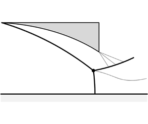
To describe the time history of the Mach stem, Li et al. (Reference Li, Gao and Wu2011) divided the transition process into a multiple-interaction stage and a pure-MR stage based on the evolution of the flow structure. Figure 5 gives a schematic illustration of these two stages. At the initial stage of the transition, the flow field appears as a multiple-interaction structure. This structure was first observed in the numerical simulations of Kudryavtsev et al. (Reference Kudryavtsev, Khotyanovsky, Ivanov and Vandromme2002) and explained by Li et al. (Reference Li, Gao and Wu2011), as illustrated in figure 5(a). The overall structure is still RR, and a the Mach stem (m) appears locally near the reflection point. The appearance of the Mach stem forms a three-shock structure with the incident (i) and reflected (r) shock waves corresponding to the MR. Here, the RR structure still exists downstream of the triple point (T). The corresponding reflected shock wave (r $'$) of the RR structure interferes with r and results in another triple point (O), a transmitted shock wave (r $''$) and a slip line (s $'$). The transmitted shock wave r $''$ further interferes with the slip line (s) emitted from the triple point T. This prevents it from intersecting with the reflecting surface, as this is physically impossible for streamlines. This is true even though, based on the CFD results shown in figure 2, the point N at which r $''$ and s intersect is close to the reflecting surface. In the mathematical description, Li et al. (Reference Li, Gao and Wu2011) assumed that point N is on the reflecting surface. Thus the flow from the Mach stem is used to grow the control volume TNG. As the Mach stem grows, the initial formation of the sonic throat indicates that the flow field enters the pure-MR stage, as assumed by Mouton & Hornung (Reference Mouton and Hornung2007). Figure 5(b) gives a schematic diagram of the configuration. This is similar to the stationary MR, except that the triple point moves upstream along the incident shock wave with velocity $V_T$. This velocity is the key parameter of the transition. The next subsubsection describes the method to determine this.

Figure 5. Schematic illustration of two dynamic configurations during the transition: (a) multiple-interaction stage, and (b) pure-MR stage.
2.2.1. Solution for the moving triple point
We start with the flow around the moving triple point. It is assumed that the flow just around the three-shock structure is pseudo-steady and satisfies the steady three-shock theory when the reference frame is attached to the triple point. The shock wave relationships and curved shock equations described by (2.1) and (2.2) still connect the flow parameters upstream and downstream of the incident shock wave (i). The incident shock wave is stationary in both the fixed and moving frames attached to the moving triple point. In contrast to the incident shock wave, the reflected shock wave (r) and Mach stem (s) remain stationary only in the moving frame.
Based on the basic shock relations and curved shock equations attached to the moving frame derived in Appendix B, the flow parameters in regions (2) and (3) are given by
 \begin{gather} \left. \begin{gathered} \frac{{{p_2}}}{{{p_1}}} = 1 + \frac{{2\gamma }}{{\gamma + 1}}
(M_{1,M}^2\sin^2{\theta _{r,M}}- 1),\\
\tan (\delta _{2,M}-\delta_{1,M}) = 2\cot {\theta _{r,M}}\frac{{M_{1,M}^2\sin^2{\theta _{r,M}} - 1}}{{M_{1,M}^2
(\gamma + \cos (2\theta _{r,M})) + 2}},\\
\frac{{{p_3}}}{{{p_0}}} = 1 + \frac{{2\gamma }}{{\gamma + 1}}(M_{0,M}^2\sin^2{\theta _{m,M}}- 1),\\
\tan (\delta _{3,M}- \delta _{0,M}) = 2\cot {\theta _{m,M}}\frac{{M_{0,M}^2\sin^2{\theta _{m,M}} - 1}}{{M_{0,M}^2(\gamma + \cos (2{\theta _{m,M}})) + 2}},\\
{p_3} = {p_2},\\ {\delta _3} = {\delta _2},\end{gathered} \right\} \end{gather}
\begin{gather} \left. \begin{gathered} \frac{{{p_2}}}{{{p_1}}} = 1 + \frac{{2\gamma }}{{\gamma + 1}}
(M_{1,M}^2\sin^2{\theta _{r,M}}- 1),\\
\tan (\delta _{2,M}-\delta_{1,M}) = 2\cot {\theta _{r,M}}\frac{{M_{1,M}^2\sin^2{\theta _{r,M}} - 1}}{{M_{1,M}^2
(\gamma + \cos (2\theta _{r,M})) + 2}},\\
\frac{{{p_3}}}{{{p_0}}} = 1 + \frac{{2\gamma }}{{\gamma + 1}}(M_{0,M}^2\sin^2{\theta _{m,M}}- 1),\\
\tan (\delta _{3,M}- \delta _{0,M}) = 2\cot {\theta _{m,M}}\frac{{M_{0,M}^2\sin^2{\theta _{m,M}} - 1}}{{M_{0,M}^2(\gamma + \cos (2{\theta _{m,M}})) + 2}},\\
{p_3} = {p_2},\\ {\delta _3} = {\delta _2},\end{gathered} \right\} \end{gather}
 \begin{gather} \left. \begin{gathered} {A_{1,r}}{P_{1,M}} + {B_{1,r}}{D_{1,M}} + {E_{1,r}}{\varGamma _{1,M}} = {A_{2,r}}{P_{2,M}} + {B_{2,r}}{D_{2,M}} + {C_{r}}{S_{a,r}},\\ A_{1,r}'{P_{1,M}} + B_{1,r}'{D_{1,M}} + E_{1,r}'{\varGamma _{1,M}} = A_{2,r}'{P_{2,M}} + B_{2,r}'{D_{2,M}} + C_{r}'{S_{a,r}},\\ {A_{0,m}}{P_{0,M}} + {B_{0,m}}{D_{0,M}} + {E_{0,m}}{\varGamma _{0,M}} = {A_{3,m}}{P_{3,M}} + {B_{3,m}}{D_{3,M}} + {C_{m}}{S_{a,m}},\\ A_{0,m}'{P_{0,M}} + B_{0,m}'{D_{0,M}} + E_{0,m}'{\varGamma _{0,M}} = A_{3,m}'{P_{3,M}} + B_{3,m}'{D_{3,M}} + C_{m}'{S_{a,m}},\\ M_3^2{P_3} = M_2^2{P_2},\\ {D_3} = {D_2}. \end{gathered} \right\} \end{gather}
The quantities with subscript  $M$ are in the moving frame (the reference frame attached to the moving triple point). Their transformation relations with the quantities in the fixed frame are
 \begin{equation} \left. \begin{gathered} V_M^2 = {\left( {V\cos \delta + {V_T}\cos {\eta _T}} \right)^2} + {\left( {V\sin \delta + {V_T}\sin {\eta _T}} \right)^2},\\ {\delta _M} = \arctan \left( {\frac{{V\sin \delta + {V_T}\sin {\eta _T}}}{{V\cos \delta + {V_T}\cos {\eta _T}}}} \right),\\ M{_M} = {V_M}\sqrt {\frac{\rho }{{\gamma p}}} ,\\ {\theta _M} = \theta + \delta - {\delta _M},\\ {P_M} = {K_{11}}P + {K_{12}}D + {K_{13}}\varGamma+K_{14},\\ {D_M} = {K_{21}}P + {K_{22}}D + {K_{23}}\varGamma+K_{24}, \\ {\varGamma _M} = {K_{31}}P + {K_{32}}D + {K_{33}}\varGamma+K_{34}. \end{gathered} \right\} \end{equation}
 The coefficients and their detailed derivations are provided in Appendix B. Here,  $V_T$ and $\eta _T$ are the magnitude and direction of the velocity of the triple point, respectively. As the triple point moves along the incident shock wave, $\eta _T=\theta _i$.
2.2.2. Determination of the triple point velocity
Due to differences in the flow structures, the velocities of the triple point in the two stages should be determined using different methods. For the pure-MR stage, the assumption of Mouton & Hornung (Reference Mouton and Hornung2007) indicates that the flow satisfies a steady-flow model when the reference frame is attached to the moving triple point. The method to determine the relationship between the velocity of the triple point and the Mach-stem height is as follows. Given a velocity  $V_T > 0$ in advance, the unsteady model (now reduced to a steady model due to the use of the moving frame) can be solved in the same way as the steady-flow model proposed in § 2.1. Thus a Mach-stem height corresponding to $V_T$ can be acquired.
For the multiple-interaction stage, we consider the triangle TNG as a control volume in which the density is constant over time (Li et al. Reference Li, Gao and Wu2011). We then apply mass conservation to determine the velocity of the triple point as
 \begin{equation} \rho_0(u_0+V_T\cos\theta_i)H_m \approx \frac{\mathrm{d}(\rho_3A_{TNG})}{\mathrm{d}t} .\end{equation}
This suggests that the mass flow rate across the Mach stem is balanced with the mass increase in the triangle TNG. In flat-shock reflections, both the reflected shock and slip line can be regarded as linear. Therefore, the area of the triangle can be calculated approximately as  $A_{TNG} = \tfrac {1}{2}H_m^2\tan {\delta _s}$. However, in curved shock reflections, the curvature of the slip line is non-negligible (illustrated in § 3.1.2). Therefore, to extend the model to curved shock reflections, we calculate the area of the triangle by integrating the shape function of the slip line derived by Shi (Reference Shi2021), who described the shape of the slip line with the quadratic function
 \begin{equation} \frac{{{D_s}}}{{2\cos^3{\delta _s}}}( {x - {x_T}} )^2 + \tan {\delta _s}\,( {x - {x_T}} ) + {H_m} - y = 0. \end{equation}
The above process establishes the relation between the position and velocity of the triple point during the whole transition process (including the pure-MR stage and the multiple-interaction stage). With this relation, the transition time corresponding to the position and velocity can be obtained by integration.
3. Results and discussion
The flow structure determined from the analytical model presented in § 2 is now studied and compared to the CFD results.
3.1. Flow structure for CMRs
3.1.1. Overall configuration
The overall structure of the flow field is studied first. Three cases of different wall curvatures under the conditions  $M_0 = 5$, $\delta _w = 26.9^\circ$ and $H_e/H_0 = 0.5$ are displayed in figure 6. This shows good agreement between the analytical (denoted by dashed red lines) and numerical results (denoted by solid black lines). Figure 6(a) illustrates the Mach number contours for the case $D_w H_0 = 0.08$. A concave shock is generated, and the corresponding reflected shock wave is close to the trailing edge. The flow field generated from a wedge ( $D_w H_0 = 0$) is shown in figure 6(b) for comparison. Distinct from the other two cases, the incident shock is linear, and the flow in front of the first expansion wave is uniform. Figure 6(c) displays an upward-curved wall with $D_w H_0 = -0.08$. The incident shock weakens as it moves downstream, and the triple point is close to the reflecting surface. These differences in flow structures are apparently caused by the curvature of the wall.

Figure 6. Comparison of the analytical configuration with the numerical results (a) case A,  $D_w H_0 = 0.08$, concave, (b) case B, $D_w H_0 = 0$, flat wall, and (c) case C, $D_w H_0 = -0.08$, convex, under the conditions $M_0 = 5$, $\delta _w = 26.9^\circ$ and $H_e/H_0 = 0.5$.
Due to the one-dimensional-flow assumption behind the Mach stem and the Kelvin–Helmholtz instability, as predicted analytically, the flow between the slip line and the reflected shock does not match well with the CFD results. Especially when the height of the Mach stem is small, the deviation between the analytical results and the CFD results seems to be large. The main reason for these deviations is the difficulty in determining the location of the sonic throat near the von Neumann transition point, as described by Gao & Wu (Reference Gao and Wu2010). We believe that another reason is the greater interference of the Kelvin–Helmholtz instability with one-dimensional flows when the slip line is closer to the reflecting surface, as shown in figure 6(c). Nevertheless, the general configuration of the flow, including the Mach stem, slip line and reflected shock wave, are well predicted. Therefore, it is appropriate to use this analytical model to study the CMR structure in planar flow.
3.1.2. Shape of the reflected shock wave and slip line
Analysis of the shape of the slip line and shock waves is helpful for understanding the action mechanism of the wall curvature. The influence mechanism of the wall curvature on the shape of the incident shock wave is simple. The concave wall generates compression waves and increases the incident shock intensity, therefore a concave incident shock is produced. Conversely, expansion waves generated from the convex wall decrease the incident shock angle, resulting in convex incident shocks.
The shape of the forward part of the reflected shock wave is also affected by these isentropic waves generated from the curved wall. Figure 7 shows the slope and curvature of the reflected shock wave for the three cases illustrated in figure 6. Before the reflected shock wave intersects the leading Mach wave generated by the trailing edge at point F, it deflects relatively slowly. After that, it starts to deviate upwards rapidly until reaching point Q, where the last Mach wave intersects it. At this point, the reflected shock wave becomes linear and the curvature dips to zero. For  $D_w \neq 0$, the curvature of the forward part of the reflected shock wave (i.e. the part before point F) is obvious due to these isentropic waves, as shown in figures 7(a,c). It is found that compression waves deflect the reflected shock downwards ( $S_{a,r}<0$), and expansion waves deflect the reflected shock upwards ( $S_{a,r}>0$). For $D_w$ = 0, the curvatures of the reflected shock remain nearly 0 before interacting with the expansion wave (figure 7b). Thus this portion of the reflected shock appears linear. An earlier investigation (Gao & Wu Reference Gao and Wu2010) indicated that the reflected shock wave remains linear before interacting with the expansion fan. Indeed, this statement is not strictly valid, even in flat-shock reflections. According to (2.2), the shock curvature is determined by the non-uniformity of the flow in front of and behind the wave. For flat-shock MRs, the flow upstream of the reflected shock wave is uniform. However, the flow behind the reflected shock wave is always non-uniform due to pressure variations in quasi-one-dimensional flows under the slip line. Therefore, the reflected shock wave is nonlinear before it interacts with the expansion fan in flat-shock MRs. This is also confirmed by the analytical results, as shown in figure 7(d). There is a slight curvature in the front portion of the reflected shock wave, while the incident shock is linear. This curvature has also been observed by Bai & Wu (Reference Bai and Wu2017). Neglecting the curvature of the forward part of the reflected shock wave might be one cause for deviations between the previous analytical models and the CFD results.

Figure 7. Slope and curvature of the analytical reflected shock wave, (a) case A,  $D_w H_0= 0.08$, (b) case B, $D_w H_0 = 0$, (c) case C, $D_w H_0= -0.08$, under the conditions $M_0 = 5$, $\delta _w = 26.9^\circ$, $H_e/H_0 = 0.5$. (d) Comparison of the reflected shock wave curvature for the three cases.
After interaction with the reflected shock wave, isentropic waves generated on the curved wall will cross it and further affect the shape of the slip line. Figure 8 provides the slope and curvature of the analytical slip line. For the flat incident shock (figure 8b), the slip line is first convex and then concave with an inflection point B. At this point, the leading transmitted Mach wave generated by the trailing edge intersects the slip line, and the curvature  $D_s$ mutates abruptly from negative to positive. The slip line deflects continuously upwards and becomes horizontal at point P, where the deflection angle is exactly zero. This rule also applies when the incident shock is concave, except that the free section of the slip line (i.e. the slip line before point B) is more convex. This suggests the possibility of inverse Mach reflection (i.e. the slip line is deflected upwards at the triple point) in curved shock reflections, while it is impossible for flat shock reflections (Ben-Dor Reference Ben-Dor2007). The situation is more complicated for a convex incident shock. As displayed in figure 8(c), the slip line is initially concave, transforms to convex between points T and B, and then develops with the above rule. These differences are exactly attributed to the interactions between the transmitted isentropic waves generated from the curved wall and the slip line.

Figure 8. Slope and curvature of the analytical slip line: (a) case A,  $D_w H_0= 0.08$, (b) case B, $D_w H_0 = 0$, (c) case C, $D_w H_0= -0.08$, under the conditions $M_0 = 5$, $\delta _w = 26.9^\circ$, $H_e/H_0 = 0.5$.
3.1.3. Mach-stem height
The variation of the shapes of the slip line and the shock waves will eventually be reflected in the variation of the Mach-stem height, which is a key parameter in MRs. In this subsubsection, the Mach-stem height will be studied quantitatively. A comparison of the normalized Mach-stem height  $H_m/H_0$ between the present analytical results and those of Bai & Wu (Reference Bai and Wu2017), Gao & Wu (Reference Gao and Wu2010), Mouton & Hornung (Reference Mouton and Hornung2007) and Li & Ben-Dor (Reference Li and Ben-Dor1997), as well as the CFD results of this work and from Gao & Wu (Reference Gao and Wu2010) for flat-shock MRs, are provided in table 1. In addition, three cases of CMRs are added to the table.
Table 1. Mach-stem heights for various conditions.

For flat-shock MRs, the difference between theory and the CFD of the current model appears to be smaller than for earlier theories for most conditions. This can be interpreted as resulting from the influence of the waves generated over the slip line being ignored either partially or entirely by previous approaches (as illustrated in § 3.1.2). Moreover, for special cases of flat-shock reflection, the heights predicted by Gao & Wu (Reference Gao and Wu2010) are also close to the CFD results, and the analytical model is much simpler than that presented here. However, the advantage of the current model is that it has a similar precision for CMRs, as seen from the last three rows of table 1.
Figure 9 further compares the present results with those of Gao & Wu (Reference Gao and Wu2010), Mouton & Hornung (Reference Mouton and Hornung2007) and Li & Ben-Dor (Reference Li and Ben-Dor1997), and the current CFD results for flat-shock MRs. We maintain a fixed wedge angle in figure 9(a), and a fixed free-stream Mach number in figure 9(b). There is good agreement between the current predictions and the CFD results, especially for large Mach-stem heights.

Figure 9. Comparisons of the current non-dimensional Mach-stem height with those in Gao & Wu (Reference Gao and Wu2010), Mouton & Hornung (Reference Mouton and Hornung2007) and Li & Ben-Dor (Reference Li and Ben-Dor1997), and the current numerical results ( $w/H_0 = 1.1$) for flat-shock MRs ( $D_w = 0$): (a) $\delta _w = 28^\circ$, and (b) $M_0 = 4.5$.
For CMRs, we studied the relationship between the wall curvature and the Mach-stem height both numerically and analytically, as shown in figure 10. The initial deflection angle  $\delta _w$ is fixed in figure 10(a), and the coordinates of the trailing edge are fixed in figure 10(b) (the fixed values are different at different Mach numbers). In figure 10(a), the Mach-stem height increases nearly linearly. This is caused by the dual effects of the changes in incident shock angle and the slip line shape. Increasing the wall curvature results in increasing incident shock wave intensity and downward deflection of the slip line. This hinders the formation of the sonic throat and increases the Mach-stem height. For cases with the same trailing edge, as shown in figure 10(b), the height of the Mach stem also shows an increasing trend as the wall curvature increases.

Figure 10. Comparisons of the current non-dimensional Mach-stem height with the numerical results ( $H_e/H_0 = 0.5$) for CMRs: (a) fixed initial deflection angle ( $\delta _w = 26^\circ$ while $M_0 = 4.5$, and $\delta _w = 28^\circ$ while $M_0 = 6$); and (b) fixed wedge-tail coordinates ( $X_e = 0.1025$ while $M_0 = 4.5$, and $X_e = 0.0940$ while $M_0 = 6$).
3.2. Time history of RR-to-MR transition
The time evolution of the Mach stem during the RR-to-MR transition is studied in this subsection to analyse the formation mechanism of the MR flow field.
3.2.1. Flat-shock transition
For a better understanding of curved shock transitions, we first study the transitions of flat shocks. Consider the case with  $M_0 = 5$, $\delta _w = 26.9^\circ$, $w/H_0 = 1.1$ and $D_w H_0 = 0$. The time evolution of the triple point as predicted by the model described in § 2.2 is displayed in figure 11 alongside the numerical results. The results obtained from the models of Mouton & Hornung (Reference Mouton and Hornung2007) and Li et al. (Reference Li, Gao and Wu2011) are also displayed. The Mach contours obtained from CFD at a series of instants during the transition process are shown in figure 12.

Figure 11. Evolutions of the triple point from the analytical model and CFD for a flat incident shock ( $M_0 = 5$, $\delta _w = 26.9^\circ$, $D_w H_0 = 0$, $w/H_0 = 1.1$). (a) Mach-stem height as a function of time; (b) relationship between the triple point velocity and the Mach-stem height; and (c) triple point velocity as a function of time.

Figure 12. Instantaneous representations of the Mach contours during the RR-to-MR transition triggered by an upstream density disturbance for a flat incident shock ( $M_0 = 5$, $\delta _w = 26.9^\circ$, $D_w H_0=0$, $H_e/H_0 = 0.5023$).
For flat-shock reflections, the analytical model indicates that the multiple-interaction stage is self-similar. Therefore, the velocity of the triple points is constant at the initial stage of the transition, as shown in figure 11 (where  $a_0$ is the speed of sound for the incoming flow). In the pure-MR stage, the velocity of the triple point gradually decreases to zero with the Mach-stem height. We also observe that for flat-shock reflections, the velocity of the predicted triple point is mostly consistent with that of Li et al. (Reference Li, Gao and Wu2011). This is because the model of the pure-MR stage established by Li et al. (Reference Li, Gao and Wu2011) is based on the steady model of Gao & Wu (Reference Gao and Wu2010). According to the analysis in § 3.1.3, the stable Mach-stem heights predicted from the current steady model and by Gao & Wu (Reference Gao and Wu2010) are both close to the CFD results for flat-shock MRs. Generally, both results agree much better with CFD than those of Mouton & Hornung (Reference Mouton and Hornung2007); this is because they did not model the multiple-interaction stage.
The numerical results indicate that the triple point moves with a velocity that first increases and then decreases. The velocity reaches its maximum at time  $t_m$, and the corresponding Mach contours are displayed in figure 12(e). The reflected shock corresponding to the MR has just entered the influence area of the expansion fan at this moment. Accordingly, the flow fields before and after $t_m$ should be analysed. Here, $\phi$ denotes the ratio of the mass flow rate out of the control volume TNG from the gap between the slip line and the reflecting surface to that into the control volume through the Mach stem. Before $t_m$, as shown in figures 12(b–d), the deflection point of the slip line is close to the reflecting surface; thus the mass flow ratio $\phi$ is close to 0. This means that nearly all of the flow from the Mach stem is used to grow the control volume. Therefore, the velocity of the triple point is relatively large at this stage. After $t_m$, the influence of the expansion waves deflects the slip line upwards. The flow out from the right-hand side of the control volume gradually increases. This leads to a velocity decrease in the triple point until the sonic throat is fully formed ( $\phi = 1$) and the flow field stabilizes.
Some new explanations for the two stages of the simplified model are given based on the above findings and analyses. The multiple-interaction stage corresponds to the initial moment of the transition at which  $\phi$ is close to 0. The pure-MR stage models the state in which the flow field tends to be stable and $\phi$ is close to 1. The envelope of the $V_T$– $H_M$ curves corresponding to the two states simulates the time history of the Mach-stem height during the transition process, and the effects of the expansion waves and changes in the flow ratio are ignored. Nevertheless, the results plotted in figure 11 show that the simplified method can generally simulate the trends of the triple point.
3.2.2. Curved shock transition
A discussion on the transition process of the curved shock further illustrates the analysis in the previous subsubsection. We consider the case with  $M_0 = 5$, $\delta _w = 22.0^\circ$, $H_e/H_0 = 0.5$ and $D_w H_0 = 0.08$ to analyse the transition of curved shock reflection. Figure 13 illustrates the time evolution of the triple point. The corresponding Mach contours are given in figure 14. The time evolution of the Mach stem in the pure-MR stage is similar to the case for the flat incident shock. However, during the multiple-interaction stage, the magnitude of the velocity of the triple point is no longer a constant; it varies with the Mach-stem height, as it should on a concave wall. The weakening of the incident shock wave leads to a decreased deflection angle for the slip line and an increased control volume area as the triple point moves upstream. Therefore, this is no longer a self-similar stage. The increased relative area of the control body instead decreases the velocity of the triple point at larger Mach stems. This process is opposite to that with a convex wall.

Figure 13. Evolution of the triple point from both the analytical model and CFD for a concave incident shock ( $M_0 = 5$, $\delta _w = 22.0^\circ$, $D_w H_0 = 0.08$, $H_e /H_0 = 0.5$). (a) Mach-stem height as a function of time; (b) relationship between the triple point velocity and the Mach-stem height; and (c) triple point velocity as a function of time.

Figure 14. Instantaneous representations of the Mach contours during the RR-to-MR transition triggered by an upstream density disturbance for a concave incident shock ( $M_0 = 5$, $\delta _w = 22.0^\circ$, $D_w H_0=0.08$, $H_e/H_0 = 0.5$).
The influence of compression or expansion waves, which are more complicated in non-uniform flow, is neglected. Therefore, the agreement between the analytical and CFD results for curved shock reflections is not as good as that for flat-shock reflections, even though the curvature of the slip line is considered. Nevertheless, the analysis based on the analytical results still reflects the trend of triple point motion. This is evidenced by the numerical results shown in figure 13. The results show that the velocity of the triple point does not tend to increase at the initial moment of the transition. Examination of the analytical results suggests that this is due to the impact of the varying incident shock angle and the decreased  $\phi$ as caused by the compression waves generated on the concave wall.
3.2.3. Transition-time analysis
Although the time evolution predicted by the theoretical model deviates from that calculated from the analytical method, it is sufficient for macroscopic law analyses. Therefore, in this subsubsection, the model is used to analyse the relationship between the transition time and the wall curvature. Figure 15 shows the time evolution of the Mach-stem height for varying wall curvatures, with fixed  $M_0$ and initial deflection angle ${\delta _w}$. We observe that the Mach-stem heights are sensitive to the wall curvature in the multiple-interaction stage. With a decreased curvature, the growth rate of the Mach stem slows down and the stationary height decreases.

Figure 15. Evolution of the Mach stem as a function of time ( $M_0 = 5$, $\delta _w = 26.5^\circ$, $H_e /H_0 = 0.5$).
We use  $t^*$ and $t_c$ to denote the times of the entire transition process and the multiple-interaction stage, respectively. Table 2 provides the non-dimensional characteristic times $t^*/(H_0/a_0)$ and $t_c /(H_0/a_0)$, the non-dimensional average speed of the triple point during the entire transition process $H_m/(t^* a_0)$, and the time proportion of the multiple-interaction stage $t_c/t^*$, for various inflow conditions. To control the variables to the greatest extent, we adjust the boundary conditions so that the stable Mach-stem heights in these cases are the same. Li et al. (Reference Li, Gao and Wu2011) defined the transition time $t^*$ as the time from the initial instance of the transition to that at which the Mach-stem height is 95 % of the stable value. However, figures 11 and 13 indicate that defining the transition time in this way is not reasonable, as the last 5 % of the height may require a significant time. With the analytical model, the time taken for the Mach stem to reach the stable height can be obtained and defined as the transition time $t^*$. The table indicates that for $H_e/H_0 = 0.5$, the times for both the entire transition process and the multiple-interaction stage are sensitive to the inflow Mach number. Increasing the inflow Mach number for a fixed Mach-stem height reduces the transition time and increases the average velocity of the triple point during the entire transition process. When the incoming Mach number is 4, the multiple-interaction stage occupies approximately $1/5$ of the total transition time. This proportion decreases and reaches approximately $1/8$ when $M_0=6$.
Table 2. Transition times for cases with the same Mach-stem height under different conditions.

In addition to the Mach number of the incoming flow, the transition time is also affected by the wall curvature, although the extent of this influence is much smaller. We observe that when the curvature is negative, the corresponding transition time is less than that for the flat shock, which increases the absolute value of the curvature. Conversely, the transition time of the concave shock is longer than that of the flat shock. This is consistent with the analysis in the previous section. We believe that this is the result of isentropic waves generated from the wall.
4. Conclusion
In this paper, the configurations of CMRs and the time evolution of the RR-to-MR transition were studied numerically and analytically. The analytical model agrees well with the CFD results when considering the global structure of the flow field. This includes the slip line, reflected shock wave, Mach stem and triple point. In CMRs, the height of the Mach stem depends not only on the strength of the incident shock wave but also on the wall curvature. The wall produces Mach waves, and these interact with shock waves and the slip line, and affect the height of the Mach stem. The influence mechanisms can be expressed as compression waves that hinder the formation of the sonic throat to increase the Mach-stem height. Expansion waves accelerate the formation of the sonic throat and decrease the height of the Mach stem.
For the transition process, the shock relationships and curved shock equations in the moving frame were studied. For curved shock transitions, the moving velocity of the triple point depends greatly on the Mach-stem height during the multiple-interaction stage. The analysis also showed that the transition time depends not only on the velocity of the incoming flow but also on the curvature of the wall. It appears that concave shock waves transition faster than convex shock waves. As the compression waves (including the incident shock wave) deflect the slip line downwards, the reduction of the area and mass flow ratio of the control volume finally increases the velocity of the triple point. In contrast, expansion waves have the effect of decreasing the velocity of the triple point.
Funding
We would like to acknowledge the support of the National Natural Science Foundation of China (NSFC, grant nos U20A2069, U21B6003 and 12202372), the Fundamental Research Funds for the Central Universities (20720220094) and project 1912. We are also grateful for the support of the open-source program AMROC: http://www.vtf.website/.
Declaration of interests
The authors report no conflict of interest.
Appendix A. Numerical methods
The numerical simulations in this paper are based on AMROC (Adaptive Mesh Refinement in Object-Oriented C++) (Deiterding Reference Deiterding2011; Laurence & Deiterding Reference Laurence and Deiterding2011), which improves the calculation efficiency with a high grid resolution (refer to the website for details: http://rdeiterding.website/html/pub.htm). In this work, only inviscid flow is considered, and the hybrid Roe solver for the Euler equations is used to solve Riemann problems along one data slice. The scheme is blended with the Harten–Lax–Van Leer scheme for robustness. A multi-dimensional entropy correction is used to prevent the carbuncle phenomenon. The slip boundary condition is used on the wedge surface and the reflecting surface; the left boundary models the supersonic inflow condition. The other boundaries are interpolated under the assumption of zero first-order derivatives over all flow parameters. We have
 \begin{equation} \left. \begin{gathered}
\frac{{{p_1}}}{{{p_0}}} = 1 + \frac{{2\gamma }}{{\gamma +
1}}\left( {M_0^2\sin^2{\theta _i} - 1} \right),\\ \tan
( {{\delta _1} - {\delta _0}} ) = 2\cot
{\theta _i}\,\frac{{M_0^2\sin^2{\theta _i} -
1}}{{M_0^2\left[ {\gamma + \cos ( {2{\theta _i}}
)} \right] + 2}},\\ \frac{{{p_4}}}{{{p_2}}} = 1 +
\frac{{2\gamma }}{{\gamma + 1}}\left(
{M_{dist}^{\rm{2}}\sin^2{\theta _{refr}} - 1}
\right),\\ \tan ( {{\delta _4} - {\delta _2}}
) = 2\cot {\theta
_{refr}}\,\frac{{M_{dist}^2\sin^2{\theta _i} -
1}}{{M_{dist}^2\left[ {\gamma + \cos \left( {2{\theta
_{refr}}} \right)} \right] + 2}},\\ {\delta _3} - \sqrt
{\frac{{\gamma + 1}}{{\gamma - 1}}} \arctan \sqrt {\left(
{\frac{{\gamma - 1}}{{\gamma + 1}}} \right)\left( {M_3^2 -
1} \right)} + \arctan \sqrt {M_3^2 - 1}\\ ={\delta _1} -
\sqrt {\frac{{\gamma + 1}}{{\gamma - 1}}} \arctan \sqrt
{\left( {\frac{{\gamma - 1}}{{\gamma + 1}}} \right)\left(
{M_1^2 - 1} \right)} + \arctan \sqrt {M_1^2 - 1} ,\\
\frac{{{p_3}}}{{{p_1}}} = {\left\{ {\frac{{1 + \left[
{\left( {\gamma - 1} \right)/2} \right]M_1^2}}{{1 + \left[
{\left( {\gamma - 1} \right)/2} \right]M_3^2}}}
\right\}^{\gamma /\left( {\gamma - 1} \right)}},\\ {p_3} =
{p_4},\quad {\delta _3} = {\delta _4}.
\end{gathered} \right\}
\end{equation}
\begin{equation} \left. \begin{gathered}
\frac{{{p_1}}}{{{p_0}}} = 1 + \frac{{2\gamma }}{{\gamma +
1}}\left( {M_0^2\sin^2{\theta _i} - 1} \right),\\ \tan
( {{\delta _1} - {\delta _0}} ) = 2\cot
{\theta _i}\,\frac{{M_0^2\sin^2{\theta _i} -
1}}{{M_0^2\left[ {\gamma + \cos ( {2{\theta _i}}
)} \right] + 2}},\\ \frac{{{p_4}}}{{{p_2}}} = 1 +
\frac{{2\gamma }}{{\gamma + 1}}\left(
{M_{dist}^{\rm{2}}\sin^2{\theta _{refr}} - 1}
\right),\\ \tan ( {{\delta _4} - {\delta _2}}
) = 2\cot {\theta
_{refr}}\,\frac{{M_{dist}^2\sin^2{\theta _i} -
1}}{{M_{dist}^2\left[ {\gamma + \cos \left( {2{\theta
_{refr}}} \right)} \right] + 2}},\\ {\delta _3} - \sqrt
{\frac{{\gamma + 1}}{{\gamma - 1}}} \arctan \sqrt {\left(
{\frac{{\gamma - 1}}{{\gamma + 1}}} \right)\left( {M_3^2 -
1} \right)} + \arctan \sqrt {M_3^2 - 1}\\ ={\delta _1} -
\sqrt {\frac{{\gamma + 1}}{{\gamma - 1}}} \arctan \sqrt
{\left( {\frac{{\gamma - 1}}{{\gamma + 1}}} \right)\left(
{M_1^2 - 1} \right)} + \arctan \sqrt {M_1^2 - 1} ,\\
\frac{{{p_3}}}{{{p_1}}} = {\left\{ {\frac{{1 + \left[
{\left( {\gamma - 1} \right)/2} \right]M_1^2}}{{1 + \left[
{\left( {\gamma - 1} \right)/2} \right]M_3^2}}}
\right\}^{\gamma /\left( {\gamma - 1} \right)}},\\ {p_3} =
{p_4},\quad {\delta _3} = {\delta _4}.
\end{gathered} \right\}
\end{equation}
To trigger the RR-to-MR transition, we introduce a localized density disturbance upstream of the reflection point, following the approach of Li et al. (Reference Li, Gao and Wu2011). The density of the lower five calculation cells that belong to the incoming flow (left) boundary is varied by  $\Delta \rho$ (figure 16a). In this way, the Mach number in the disturbed layer becomes $M_{dist} = M_0 \sqrt {1+\Delta \rho /\rho _0 }$. The disturbance is kept constant for a certain time $T = 0.1H_0 /a_0$ until the undisturbed incoming flow conditions are restored. When the disturbance propagates downstream and reaches the reflection point, the spatial Riemann problem shown in figure 16(b) occurs. The structure is similar to the triple point of the MR except that the reflected shock is replaced with an expansion fan. The angle of the refracted shock can be determined easily analytically by solving (A1). Through the proper selection of $\Delta \rho$, the refracted shock angle $\theta _{refr}$ can exceed the detachment angle $\theta _D$ and induce the transition. The level of density disturbance needed for the RR-to-MR transition can be evaluated directly, and the results are given in figure 16(c).

Figure 16. Schematic illustration of localized density disturbance: (a) upstream density disturbance; (b) spatial Riemann problem; and (c) threshold-level contour lines of the localized density disturbance.
The mesh is refined carefully near points with fine structures using the block-structured adaptive mesh-refinement technique proposed by Berger & Colella (Reference Berger and Colella1989). The refinement factor  $r_i$ is set to 2, 2 and 4. The max time step is set to $10^{-4}H_0/a_0$. Figure 17 displays the Mach contours during the transition using two grid densities ( $300 \times 120$ on level 4, and $450 \times 180$ on level 4) for $M_0 = 4$, $D_w H_0 = -0.08$, $\theta _w = 20^\circ$ and $H_e/H_0 = 0.5$. Although slight differences exist in terms of the flow details, the main flow structures in the present study of the two dense grid numbers are similar and can be well captured.

Figure 17. Instantaneous representations of the Mach contours for the RR-to-MR transition for  $M_0 = 4$, $D_w H_0 = -0.08$, $\delta _w = 20^\circ$ and $H_e/H_0 = 0.5$. The grid is $300 \times 120$ in (a–d), and $450 \times 180$ in (e–h).
Figure 18 displays the time evolutions of the triple points under the different grids and refinement levels. The results show good agreement when the number of grid points is greater than  $300 \times 120$ and the refinement level is above 3. Therefore, we use grid $300 \times 120$ or denser, and refinement level 4, throughout the paper.

Figure 18. Time evolution of the Mach-stem height during the transition using different grids and refinement levels for  $M_0 = 4$, $D_w H_0 = -0.08$, $\delta _w = 20^\circ$, and $H_e/H_0 = 0.5$.
Appendix B. Shock wave relations and curved shock equations in the moving frame
The classical shock relations and the curved shock equation for a fixed frame are provided in § 2.1.1. To build the flow model during the transition, the connections for the flow quantities between the fixed and moving frames are derived. The shock wave relationship and curved shock equations in the moving frame are provided in (B11) and (B12). Here, the subscript  $M$ denotes the quantities with respect to the moving reference frame, which moves at speed $V_T$ in the direction $\eta _T$. The flow quantities in the reference frame are related to the parameters in the fixed frame as
 \begin{equation} \left. \begin{gathered} V_M^2 = {\left( {V\cos \delta + {V_T}\cos {\eta _T}} \right)^2} + {\left( {V\sin \delta + {V_T}\sin {\eta _T}} \right)^2},\\ {\delta _M} = \arctan \left( {\frac{{V\sin \delta + {V_T}\sin {\eta _T}}}{{V\cos \delta + {V_T}\cos {\eta _T}}}} \right),\\ M{_M} = {V_M}\sqrt {\frac{\rho }{{\gamma p}}} ,\\ {\theta _M} = \theta + \delta - {\delta _M}. \end{gathered} \right\} \end{equation}
Equations (B1) provide the relationships for only the velocity, deflection angle, Mach number and shock angle. To study the high-order flow parameters of the flow field, CST in the moving reference frame should be included. The connections between the pressure gradient, streamline curvature and vorticity in the two reference frames provide the moving and fixed frames. By definition, the pressure gradient, streamline curvature and vorticity in the moving frame are given by
 \begin{equation} \left. \begin{gathered} {P_M} = \frac{1}{\rho V_M^2}\,\frac{{\partial p}}{{\partial {s_M}}},\\ {D_M} = \frac{{\partial {\delta _M}}}{{\partial {s_M}}},\\ {\varGamma _M} = \frac{1}{{{V_M}}}\,\frac{{\partial {V_M}}}{{\partial {n_M}}} - {D_M}. \end{gathered} \right\} \end{equation}
Replacing  $V_M$ and $\delta _M$ by the quantities with respect to the fixed frame gives
 \begin{equation} \left. \begin{aligned} {P_M} & = \frac{{V^2}}{{{V_M^2}}}\,\frac{1}{\rho {V^2}}\,\frac{{\partial p}}{{\partial {s_M}}},\\ {D_M} & = \frac{{\partial \left[ {\arctan \left( {\dfrac{{V\sin \delta + {V_T}\sin {\eta _T}}}{{V\cos \delta + {V_T}\cos {\eta _T}}}} \right)} \right]}}{{\partial {s_M}}}\\ & = \frac{{( {V\cos \delta + {V_T}\cos {\eta _T}} )\sin \delta - ( {V\sin \delta + {V_T}\sin {\eta _T}} )\cos \delta }}{{( {1 + \tan^2{\delta _M}} ){{( {V\cos \delta + {V_T}\cos {\eta _T}} )}^2}}}\,\frac{{\partial V}}{{\partial {s_M}}}\\ & \quad + \frac{{( {V\cos \delta + {V_T}\cos {\eta _T}} )V\cos \delta + ( {V\sin \delta + {V_T}\sin {\eta _T}} )V\sin \delta }}{{( {1 + \tan^2{\delta _M}} ){{( {V\cos \delta + {V_T}\cos {\eta _T}} )}^2}}}\,\frac{{\partial \delta }}{{\partial {s_M}}},\\ {\varGamma _M} & = \frac{1}{{{V_M}}}\,\frac{{\partial \left[ {{{( {V\cos \delta + {V_T}\cos {\eta _T}} )}^2} + {{( {V\sin \delta + {V_T}\sin {\eta _T}} )}^2}} \right]}}{{\partial {n_M}}} - {D_M}\\ & = \frac{{V + {V_T}\cos \delta \cos {\eta _T} + {V_T}\sin \delta \sin {\eta _T}}}{{V_M^2}}\,\frac{{\partial V}}{{\partial {n_M}}}\\ & \quad +\frac{{V{V_T}\sin \delta \cos {\eta _T} + V{V_T}\cos \delta \sin {\eta _T}}}{{V_M^2}}\,\frac{{\partial \delta }}{{\partial {n_M}}} - {D_M}. \end{aligned} \right\} \end{equation}
Further simplification gives
 \begin{equation} \left. \begin{aligned} {P_M} & = \frac{{V^2}}{{{V_M^2}}}\,\frac{1}{\rho {V^2}}\,\frac{{\partial p}}{{\partial {s_M}}},\\ {D_M} & = \frac{{{V_T}\sin ( {\delta - {\eta _T}} )}}{{( {1 + \tan^2{\delta _M}} ){{( {V\cos \delta + {V_T}\cos {\eta _T}} )}^2}}}\,\frac{{\partial V}}{{\partial {s_M}}}\\ & \quad + \frac{{{V^2} + V{V_T}\cos ( {\delta - {\eta _T}} )}}{{( {1 + \tan^2{\delta _M}} ){{( {V\cos \delta + {V_T}\cos {\eta _T}} )}^2}}}\,\frac{{\partial \delta }}{{\partial {s_M}}},\\ {\varGamma _M} & = \frac{{V + {V_T}\cos ( {\delta - {\eta _T}} )}}{{V_M^2}}\,\frac{{\partial V}}{{\partial {n_M}}} + \frac{{V{V_T}\sin ( {\delta + {\eta _T}} )}}{{V_M^2}}\,\frac{{\partial \delta }}{{\partial {n_M}}} - {D_M}. \end{aligned} \right\} \end{equation}
The derivatives of any quantity with respect to distance along and normal to the streamline in the moving frame can be expressed in terms of the two derivatives along and normal to the streamline in the fixed frame as
 \begin{equation} \left. \begin{aligned} & \left( {\frac{{\partial \bullet }}{{\partial {s_M}}}} \right) = \left( {\frac{{\partial \bullet }}{{\partial s}}} \right)\cos ( {{\delta _M} - \delta } ) + \left( {\frac{{\partial \bullet }}{{\partial n}}} \right)\sin ( {{\delta _M} - \delta } ),\\ & \left( {\frac{{\partial \bullet }}{{\partial {n_M}}}} \right) ={-} \left( {\frac{{\partial \bullet }}{{\partial s}}} \right)\sin ( {{\delta _M} - \delta } ) + \left( {\frac{{\partial \bullet }}{{\partial n}}} \right)\cos ( {{\delta _M} - \delta } ). \end{aligned} \right\} \end{equation}
This produces
 \begin{equation} \left. \begin{aligned} {P_M} & = \frac{{V^2}}{{{V_M^2}}}\,\frac{1}{\rho {V^2}}\left[ {\frac{{\partial p}}{{\partial s}}\cos ({\delta _M} - \delta ) + \frac{{\partial p}}{{\partial n}}\sin ({\delta _M} - \delta )} \right],\\ {D_M} & = \frac{{{V_T}\sin ( {\delta - {\eta _T}} )}}{{( {1 + \tan^2{\delta _M}} ){{( {V\cos \delta + {V_T}\cos {\eta _T}} )}^2}}}\left[ {\frac{{\partial V}}{{\partial s}}\cos ({\delta _M} - \delta ) + \frac{{\partial V}}{{\partial n}}\sin ({\delta _M} - \delta )} \right]\\ & \quad + \frac{{{V^2} + V{V_T}\cos ( {\delta - {\eta _T}} )}}{{( {1 + \tan^2{\delta _M}} ){{( {V\cos \delta + {V_T}\cos {\eta _T}} )}^2}}}\left[ {\frac{{\partial \delta }}{{\partial s}}\cos ({\delta _M} - \delta ) + \frac{{\partial \delta }}{{\partial n}}\sin ({\delta _M} - \delta )} \right],\\ {\varGamma _M} & = \frac{{V + {V_T}\cos ( {\delta - {\eta _T}} )}}{{V_M^2}}\left( { - \frac{{\partial V}}{{\partial s}}\sin ({\delta _M} - \delta ) + \frac{{\partial V}}{{\partial n}}\cos ({\delta _M} - \delta )} \right)\\ & \quad +\frac{{V{V_T}\sin ( {\delta + {\eta _T}} )}}{{V_M^2}}\left( { - \frac{{\partial \delta }}{{\partial s}}\sin ({\delta _M} - \delta ) + \frac{{\partial \delta }}{{\partial n}}\cos ({\delta _M} - \delta )} \right) - {D_M}. \end{aligned} \right\} \end{equation}
 The derivatives  ${\partial \bullet }/{\partial s}$ and ${\partial \bullet }/{\partial n}$ can be expressed as
 \begin{equation}
\left.\begin{aligned}
\frac{{\partial p}}{{\partial s}} &= \rho {V^2}P, & \frac{{\partial p}}{{\partial n}} &={-} \rho {V^2}D,\\
\frac{{\partial V}}{{\partial s}} &={-} PV, &\frac{{\partial V}}{{\partial n}} &={-} V\left( {D - \varGamma } \right),\\
\frac{{\partial \delta }}{{\partial s}} &= D, & \frac{{\partial \delta }}{{\partial n}} &={-}( {{M^2} - 1} )P - j\,\frac{{\sin \delta }}{y}.
\end{aligned} \right\} \end{equation}
\begin{equation}
\left.\begin{aligned}
\frac{{\partial p}}{{\partial s}} &= \rho {V^2}P, & \frac{{\partial p}}{{\partial n}} &={-} \rho {V^2}D,\\
\frac{{\partial V}}{{\partial s}} &={-} PV, &\frac{{\partial V}}{{\partial n}} &={-} V\left( {D - \varGamma } \right),\\
\frac{{\partial \delta }}{{\partial s}} &= D, & \frac{{\partial \delta }}{{\partial n}} &={-}( {{M^2} - 1} )P - j\,\frac{{\sin \delta }}{y}.
\end{aligned} \right\} \end{equation}
With these substitutions,  $P_M$, $D_M$ and $\varGamma _M$ become
 \begin{equation} \left. \begin{aligned} {P_M} & = \frac{{V^2}}{{{V_M^2}}}\,P\cos ({\delta _M} - \delta ) - \frac{{V^2}}{{{V_M^2}}}\,D\sin ({\delta _M} - \delta ),\\ {D_M} & = \frac{{{V_T}\sin ( {\delta - {\eta _T}} )}}{{( {1 + \tan^2{\delta _M}} ){{( {V\cos \delta + {V_T}\cos {\eta _T}} )}^2}}}\\ & \quad \times \left[ { - PV\cos ({\delta _M} - \delta ) + V(D - \varGamma )\sin ({\delta _M} - \delta )} \right]\\ & \quad + \frac{{{V^2} + V{V_T}\cos ( {\delta - {\eta _T}} )}}{{( {1 + \tan^2{\delta _M}} ){{( {V\cos \delta + {V_T}\cos {\eta _T}} )}^2}}}\\ & \quad \times \left\{ {D\cos ({\delta _M} - \delta ) + \left[ {-( { {M^2} - 1} )P - j\,\frac{{\sin \delta }}{y}} \right]\sin ({\delta _M} - \delta )} \right\},\\ {\varGamma _M} & = \frac{{V{V_T}\sin ( {\delta + {\eta _T}} )}}{{V_M^2}}\left\{ { - D\sin ({\delta _M} - \delta ) + \left[ {-( { {M^2} - 1} )P - j\,\frac{{\sin \delta }}{y}} \right]\cos ({\delta _M} - \delta )} \right\}\\ & \quad +\frac{{V + {V_T}\cos ( {\delta - {\eta _T}} )}}{{V_M^2}}\left( {PV\sin ({\delta _M} - \delta ) + V(D - \varGamma )\cos ({\delta _M} - \delta )} \right) - {D_M}. \end{aligned} \right\} \end{equation}
Collecting terms gives
 \begin{equation} \left. \begin{gathered} {P_M} = {K_{11}}P + {K_{12}}D + {K_{13}}\varGamma+K_{14},\\ {D_M} = {K_{21}}P + {K_{22}}D + {K_{23}}\varGamma+K_{24}, \\ {\varGamma _M} = {K_{31}}P + {K_{32}}D + {K_{33}}\varGamma+K_{34}, \end{gathered} \right\} \end{equation}
where
 \begin{equation} \left. \begin{aligned} {K_{11}} & = \frac{{V^2}}{{{V_M^2}}}\cos ({\delta _M} - \delta ),\\ {K_{12}} & ={-} \frac{{V^2}}{{{V_M^2}}}\sin ({\delta _M} - \delta ),\\ {K_{13}} & = 0,\\ {K_{14}} & = 0,\\ {K_{21}} & ={-} \frac{{V{V_T}\sin ( {\delta - {\eta _T}} )}}{{( {1 + \tan^2{\delta _M}} ){{( {V\cos \delta + {V_T}\cos {\eta _T}} )}^2}}}\cos ({\delta _M} - \delta )\\ & \quad - \frac{{{V^2} + V{V_T}\cos ( {\delta - {\eta _T}} )}}{{( {1 + \tan^2{\delta _M}} ){{( {V\cos \delta + {V_T}\cos {\eta _T}} )}^2}}}\,( {{M^2} - 1} )\sin ({\delta _M} - \delta ),\\ {K_{22}} & = \frac{{V{V_T}\sin ( {\delta - {\eta _T}} )}}{{( {1 + \tan^2{\delta _M}} ){{( {V\cos \delta + {V_T}\cos {\eta _T}} )}^2}}}\sin ({\delta _M} - \delta )\\ & \quad+ \frac{{{V^2} + V{V_T}\cos ( {\delta - {\eta _T}} )}}{{( {1 + \tan^2{\delta _M}} ){{( {V\cos \delta + {V_T}\cos {\eta _T}} )}^2}}}\cos ({\delta _M} - \delta ),\\ {K_{23}} & ={-} \frac{{V{V_T}\sin ( {\delta - {\eta _T}} )}}{{( {1 + \tan^2{\delta _M}} ){{( {V\cos \delta + {V_T}\cos {\eta _T}} )}^2}}}\sin ({\delta _M} - \delta ),\\ {K_{24}} & ={-} \frac{{{V^2} + V{V_T}\cos ( {\delta - {\eta _T}} )}}{{( {1 + \tan^2{\delta _M}} ){{( {V\cos \delta + {V_T}\cos {\eta _T}} )}^2}}}\,j\,\frac{{\sin \delta }}{y}\sin ({\delta _M} - \delta ),\\ {K_{31}} & ={-} \frac{{V{V_T}\sin ( {\delta + {\eta _T}} )}}{{V_M^2}}\,( {{M^2} - 1} )\cos ({\delta _M} - \delta ) + \frac{{{V^2} + V{V_T}\cos ( {\delta - {\eta _T}} )}}{{V_M^2}}\sin ({\delta _M} - \delta ),\\ {K_{32}} & ={-} \frac{{V{V_T}\sin ( {\delta + {\eta _T}} )}}{{V_M^2}}\sin ({\delta _M} - \delta ) + \frac{{{V^2} + V{V_T}\cos ( {\delta - {\eta _T}} )}}{{V_M^2}}\cos ({\delta _M} - \delta ),\\ {K_{33}} & ={-} \frac{{{V^2} + V{V_T}\cos ( {\delta - {\eta _T}} )}}{{V_M^2}}\cos ({\delta _M} - \delta ),\\ {K_{34}} & ={-} \frac{{V{V_T}\sin ( {\delta + {\eta _T}} )}}{{V_M^2}}\,j\,\frac{{\sin \delta }}{y}\cos ({\delta _M} - \delta ) - {D_M}. \end{aligned} \right\} \end{equation}
Through the above transformation, the shock relationship and curved shock equations can be written in the form of the moving frame as
 \begin{gather} \left. \begin{gathered} \frac{{{p_1}}}{{{p_0}}} = 1 + \frac{{2\gamma }}{{\gamma + 1}}\left( {M_{0,M}^2\sin^2{\theta _M} - 1} \right),\\ \frac{{{\rho _1}}}{{{\rho _0}}} = \frac{{( {\gamma + 1} )M_{0,M}^2\sin^2{\theta _M}}}{{( {\gamma - 1} )M_{0,M}^2\sin^2{\theta _M} + 2}},\\ \frac{{{V_{1,M}}}}{{{V_{0,M}}}} = \frac{{\cos {\theta _M}}}{{\cos ( {{\theta _M} - {\delta _M}} )}},\\ \tan ( {{\delta _{1,M}} - {\delta _{0,M}}} ) = 2\cot {\theta _M}\,\frac{{M_{0,M}^2\sin^2{\theta _M} - 1}}{{M_{0,M}^2\left( {\gamma + \cos ( {2{\theta _M}} )} \right) + 2}}, \end{gathered} \right\} \end{gather}
 \begin{gather} \left. \begin{gathered} {A_{0}}{P_{0,M}} + {B_{0}}{D_{0,M}} + {E_{0}}{\varGamma _{0,M}} = {A_{1}}{P_{1,M}} + {B_{1}}{D_{1,M}} + {C}{S_a},\\ A_{0}'{P_{0,M}} + B_{0}'{D_{0,M}} + E_{0}'{\varGamma _{0,M}} = A_{1}'{P_{1,M}} + B_{1}'{D_{1,M}} + C'{S_a},\\ A_{0}''{P_{0,M}} + B_{0}''{D_{0,M}} + E_{0}''{\varGamma _{0,M}} = A_{1}''{P_{1,M}} + B_{1}''{D_{1,M}} + E_{1}''{\varGamma _{1,M}} + C''{S_a}. \end{gathered} \right\} \end{gather}
The coefficients are also calculated in the moving frame.


