


1. Introduction
High Reynolds number flows tend to become hydrodynamically unstable wherein a small perturbation of the velocity field grows rapidly, resulting in a transformation of the base flow field in finite time (Drazin Reference Drazin2002). In general, instability draws energy from an organized base flow and deposits into a less-organized perturbation field. When the velocity perturbations grow to a threshold magnitude relative to the base flow, nonlinear effects set in (Reshotko Reference Reshotko1976; Morkovin Reference Morkovin1994), initiating breakdown of the base flow toward a turbulent state which is characterized by chaotic velocity fluctuations. As a flow transitions from a base laminar flow to a chaotic turbulent state, there is a significant change in the overall mass, momentum and energy transport characteristics (Pope Reference Pope2001; Monin & Yaglom Reference Monin and Yaglom2013). The study of instabilities is therefore of great importance for flows in nature and engineering.
In incompressible flows, all of the kinetic energy extracted from the mean flow by the instability-enabled production mechanism goes toward energizing the perturbation velocity field (Pope Reference Pope2001; George Reference George2013). Pressure is merely a Lagrange multiplier with the sole function of preserving a dilatation-free velocity field and hence does no work (energy transfer) on the velocity field (Pope Reference Pope2001). As a result, instability and ensuing turbulence analyses do not entail thermodynamic or internal energy considerations.
In compressible flows, the role of pressure reverts to that of a thermodynamic state variable (Anderson Reference Anderson1990). Pressure field now evolves according to a wave equation derived from an internal energy balance and equation of state (Landau & Lifshitz Reference Landau and Lifshitz1987; Lele Reference Lele1994). The change in the fundamental nature of pressure action triggers important flow–thermodynamics interactions. Most importantly, the velocity field develops a dilatational component allowing for pressure to perform work on the velocity field (or vice versa) via the pressure-dilatation mechanism. Thus additional degrees of freedom and a new component of energy (internal) enter into the instability analysis. From the perspective of energetics, the kinetic energy extracted from the mean flow can be diverted away from perturbation kinetic energy to perturbation internal energy by the pressure-dilatation mechanism (Sarkar et al. Reference Sarkar, Erlebacher, Hussaini and Kreiss1991; Sarkar Reference Sarkar1992; Praturi & Girimaji Reference Praturi and Girimaji2019; Mittal & Girimaji Reference Mittal and Girimaji2020).
The initial growth/decay of small perturbations is described by linear stability theory. Linear stability analysis (LSA) of an incompressible boundary layer shows the emergence of the Tollmien–Schlichting instability (also termed the first mode) beyond a critical Reynolds number (Schmid, Henningson & Jankowski Reference Schmid, Henningson and Jankowski2002). Akin to incompressible flows, instability in compressible boundary layers has been studied in the literature using LSA (Lees & Lin Reference Lees and Lin1946; Mack Reference Mack1984; Reed, Saric & Arnal Reference Reed, Saric and Arnal1996; Criminale, Jackson & Joslin Reference Criminale, Jackson and Joslin2018). Lees & Lin (Reference Lees and Lin1946) extended the Rayleigh stability criterion (Rayleigh Reference Rayleigh1880) to compressible flows, and established that an extremum of mean angular momentum ( $D(\bar {\rho }D\bar {U})=0$) is necessary for inviscid instability. Mack (Reference Mack1984) developed a more complete theory for boundary layers by performing extensive stability calculations. At subsonic Mach numbers, compressibility is known to have a stabilizing effect. Unlike subsonic flows, beyond $M=1$, oblique first modes are more unstable than their two-dimensional (2-D) counterparts. In addition to the first mode, at high Mach numbers a new family of instability modes coexists along with the first mode (Mack Reference Mack1984). These additional modes belong to the family of trapped acoustic waves and exist whenever there is a relative supersonic region in the flow, i.e. the relative Mach number is greater than 1. The first of these additional modes, termed the second or Mack mode, becomes the dominant instability (Mack Reference Mack1984) at $M\geq 4$ for an adiabatic flat plate. Gushchin & Fedorov (Reference Gushchin and Fedorov1990) show that the second mode instability occurs in a region where two modes of the discrete spectrum are synchronized, leading to the branching of the discrete spectrum. These discrete modes were categorized as fast ( $F$) and slow ( $S$) by Fedorov (Reference Fedorov2011) based on their asymptotic behaviour near the leading edge. The branching pattern of the discrete spectrum is dependent on the Mach number at a fixed Reynolds number (Fedorov & Tumin Reference Fedorov and Tumin2011). As a result, depending on the flow parameters, the second mode can be associated with the fast or slow mode. Extensive studies have been conducted on the effect of wall cooling for these modes (Lees & Lin Reference Lees and Lin1946; Mack Reference Mack1984; Malik Reference Malik1989; Masad, Nayfeh & Al-Maaitah Reference Masad, Nayfeh and Al-Maaitah1992; Mack Reference Mack1993). In general, cooling stabilizes the first mode while destabilizing the second mode. Consequently for cold walls, the second mode becomes the dominant instability at even lower Mach numbers. Recently, Bitter & Shepherd (Reference Bitter and Shepherd2015) have shown the existence of unstable supersonic modes at very high levels of cooling causing the flow to become unstable over a much wider range of frequencies. Malik & Anderson (Reference Malik and Anderson1991) investigated real gas effects on the stability of hypersonic boundary layers by considering disassociation of air and conclude that real gas effects stabilize the first mode while destabilizing the second mode.
At high temperatures excitation of internal modes and disassociation can lead to large deviation of the effective Prandtl number from its baseline value (Hansen Reference Hansen1958; Capitelli et al. Reference Capitelli, Colonna, Gorse and d'Angola2000). The Prandtl number for air at atmospheric pressure and extremely high temperatures can be  $0.9$ or higher, whereas at low pressures and high temperature the Prandtl number can be as low as $0.3$ (Hansen Reference Hansen1958; Capitelli et al. Reference Capitelli, Colonna, Gorse and d'Angola2000). Such combinations of extremely high temperature and low pressure can be experienced during hypersonic re-entry in the Jovian atmosphere (Seiff et al. Reference Seiff, Kirk, Knight, Young, Mihalov, Young, Milos, Schubert, Blanchard and Atkinson1998). The effect of flow parameters such as the Mach number, wall temperature and Reynolds number on compressible boundary layer stability have been studied extensively in the literature (Mack Reference Mack1984; Malik Reference Malik1989; Masad et al. Reference Masad, Nayfeh and Al-Maaitah1992; Fedorov & Tumin Reference Fedorov and Tumin2011). However, studies examining the effect of Prandtl number have been limited. Ramachandran et al. (Reference Ramachandran, Saikia, Sinha and Govindarajan2015) investigate the effect of the Prandtl number on the eigenspectrum of hypersonic boundary layers. They observe destabilization of both first and second modes with increasing Prandtl number. Moreover, their findings also suggest that the discrete spectrum branching pattern is dependent on the Prandtl number. Although the effect of the Prandtl number on instability trends and eigenspectrum branching has been discussed, the underlying physics leading to the destabilization has not been clearly explained.
Comprehensive understanding of instability at different Mach and Prandtl numbers is of much value for many engineering flows for developing predictive tools. Specifically, there is much interest in a unified reduced-order computational tool capable of accurately simulating the entire transition-to-turbulence process. This entails developing closure models for various flow mechanisms and processes contributing toward instability.
In this work, we seek to understand the flow physics underlying the effect of the Prandtl number on boundary layer instability with adiabatic walls. These effects manifest on the flow stability via the flow–thermodynamics interactions. Thus we investigate perturbation internal energy, kinetic energy and pressure–velocity interactions. We establish kinetic and internal energy levels of the first and second modes at different Mach and Prandtl numbers. The various flow–thermodynamics interactions and turbulence mechanisms contributing to first and second instability modes are also examined. We explicate the observed instability behaviour by characterizing production, pressure–strain correlation and pressure dilatation at different Mach and Prandtl numbers. The profiles of the base flow and the stresses are analysed to explain the different trends shown by the first and second modes. The results obtained by LSA are corroborated by direct numerical simulations performed using the gas kinetic method (Xu Reference Xu2001). Thus the work also leads to the validation of the kinetic-theory-based numerical scheme and computational code.
2. Governing equations and linear analysis
The compressible Navier–Stokes equations for an ideal fluid are as follows:
 $$\begin{gather} \frac{\partial \rho^*}{\partial t^*} + \frac{\partial}{\partial x_j^*} (\rho^* u_j^*) =0, \end{gather}$$
 $$\begin{gather}\frac{ \partial (\rho^* u_i^*)}{\partial t^*} + \frac{\partial (\rho^* u_i^* u_j^*)}{\partial x_j^*} ={-}\frac{\partial p^*}{\partial x_i^*} + \frac{\partial {\mathsf \tau}_{ij}^*}{\partial x_j^*}, \end{gather}$$
 $$\begin{gather}\frac{\partial}{\partial t^*} \left(\frac{p^*}{\gamma-1}\right) + \frac{\partial }{\partial x_j^*}\left(\frac{p^* u_j^*}{\gamma-1}\right) = \frac{\partial}{\partial x_j^*} \left( \kappa^* \frac{\partial T^*}{\partial x_j^*} \right) - p^* \frac{\partial u_k^*}{\partial x_k^*} + {\mathsf \tau}_{ij}^*\frac{\partial u_i^*}{\partial x_j^*}, \end{gather}$$
 $$\begin{gather}p^* = \rho^* R T^*, \end{gather}$$
where the superscript  $^{*}$ is used to denote the dimensional variables. The density of the fluid is denoted by $\rho ^*$, velocity by $u_i^*$, temperature by $T^*$ and pressure by $p^*$. Also, $\gamma$ is the specific heat ratio, $\kappa ^*$ is the coefficient of thermal conductivity, $R$ is the universal gas constant and ${\mathsf \tau} _{ij}^*$ is the viscous stress tensor given by
 \begin{equation} {\mathsf \tau}_{ij}^*=\mu^* \left(\frac{\partial u_i^*}{\partial x_j^*} +\frac{\partial u_j^*}{\partial x_i^*} \right) - \frac{2}{3}\mu^*\frac{\partial u_k^*}{\partial x_k^*}{\mathsf \delta}_{ij}. \end{equation}
The coefficient of viscosity  $\mu ^*$ is dependent on the local temperature as dictated by Sutherland's law (Sutherland Reference Sutherland1893).
The evolution of total kinetic energy ( $\rho ^*u_i^*u_i^*/2$) as obtained from the momentum equations (2.1b) is given by
 \begin{equation} \frac{ \partial (\rho^* u_i^*u_i^*/2)}{\partial t^*} + \frac{\partial (u_j^*\rho^* u_i^*u_i^*/2 )}{\partial x_j^*} = \underbrace{p^* \frac{\partial u_i^*}{\partial x_i}}_{\varPi} \underbrace{-{\mathsf \tau}_{ij}^*\frac{\partial u_i^*}{\partial x_j}}_{\epsilon} +\underbrace{\frac{\partial}{\partial x_j}[{\mathsf \tau}_{ij}^*u_i^*-p^*u_i^*{\mathsf \delta}_{ij}]}_{\mathcal{T}}.\end{equation}
Here,  $\varPi$ represents pressure dilatation, $\epsilon$ is viscous dissipation of kinetic energy and $\mathcal {T}$ is the kinetic energy transport term. From (2.1c) it is evident that the pressure-dilatation and dissipation terms couple the kinetic and internal/pressure modes. Pressure dilatation enables a reversible exchange between the internal and kinetic energies. On the other hand, the dissipation of kinetic energy to the internal mode is irreversible.
2.1. Linear stability analysis
The dimensional variables are normalized as follows:
 \begin{equation} \left.\begin{array}{c@{}} \displaystyle u_i = \dfrac{u_i^*}{U_\infty}, \quad \rho = \dfrac{\rho^*}{\rho_\infty}, \quad T = \dfrac{T^*}{T_\infty}, \quad p = \dfrac{p^*}{\rho_\infty U_\infty^2}, \\ \displaystyle x_i = \dfrac{x_i^*}{L_r}, \quad t = \dfrac{t^*U_\infty}{L_r} , \quad \mu = \dfrac{\mu^*}{\mu_\infty}, \quad \kappa = \dfrac{\kappa^*}{\kappa_\infty}, \end{array}\right\} \end{equation}
where  $U_\infty$ is the free-stream velocity, $\rho _\infty$ is the free-stream density, $T_\infty$ is the free-stream temperature and $\mu _\infty$ and $\kappa _\infty$ are the free-stream viscosity and thermal conductivity, respectively. The spatial coordinate $x_i^*$ is normalized by the Blasius length scale $L_r=\sqrt {\mu _\infty x^*/\rho _\infty U_\infty }$.
The flow variables are then decomposed into a basic state and perturbations
 \begin{equation} A=\bar{A}+A'. \end{equation}
Here,  $A$ represents the flow variables ( $u_i, \rho, p, T$). We assume a 2-D locally parallel basic state wherein the wall-normal and spanwise base velocities are zero. Moreover, the basic state properties only vary along the wall-normal direction $x_2$. A schematic of the base flow is shown in figure 1. The fluid properties, viscosity and thermal conductivity are also decomposed into a base state and perturbations. The base viscosity ( $\bar {\mu }$) is obtained from Sutherland's law of viscosity (Sutherland Reference Sutherland1893) while the base thermal conductivity ( $\bar {\kappa }$) is varied to ensure a constant Prandtl number across the boundary layer. The viscosity and thermal conductivity perturbations are expressed in terms of temperature fluctuations as
 \begin{equation} \mu'=\frac{{\rm d} \bar{\mu}}{{\rm d} \bar{T}}T';\quad \kappa'=\frac{{\rm d} \bar{\kappa}}{{\rm d} \bar{T}}T', \end{equation}
where the derivatives  $\textrm {d} \bar {\mu }/\textrm {d} \bar {T}$ and $\textrm {d} \bar {\kappa }/ \textrm {d} \bar {T}$ are also computed from Sutherland's law.

Figure 1. Schematic of the basic state for LSA and the problem set-up for direct numerical simulation (DNS). Here,  $L_{x1}$, $L_{x2}$ and $L_{x3}$ represent the domain sizes in the streamwise, wall-normal and spanwise directions, respectively, and $\delta _{99}$ denotes the 99 % boundary layer thickness.
The basic state is obtained by solving the 2-D compressible laminar flat plate boundary layer equations using the Levy–Lees similarity transformation (Rogers Reference Rogers1992). The physical coordinates ( $x_1^*, x_2^*$) are transformed to the ( $\xi$– $\eta$) space using the following relations:
 \begin{equation} \left.\begin{array}{c@{}} \displaystyle \xi=\int_0^{x_1^*} \rho_\infty\mu_\infty U_\infty \, {\rm d} x_1^*, \\ \displaystyle \eta=\dfrac{U_\infty}{\sqrt{2\xi}}\int_0^{x_2^*} \bar{\rho} \, {\rm d} x_2^*. \end{array}\right\} \end{equation}
The basic state equations in the transformed space reduce to a system of ordinary differential equations (ODEs) given by (Rogers Reference Rogers1992)
 $$\begin{gather} (Cf'')' + ff''=0, \end{gather}$$
 $$\begin{gather}\left(\frac{C}{Pr}g'\right)' + fg' + (\gamma-1)M^2Cf''^2=0. \end{gather}$$
Here, the similarity variable  $f'=\bar {U}_1$ is the non-dimensional streamwise velocity, $g=\bar {T}$ is the non-dimensional temperature, $C=\bar {\rho }\bar {\mu }$ is the Chapman–Rubesin factor, $M$ is the free-stream Mach number and $Pr$ is the Prandtl number. For an adiabatic flat plate, the set of ODEs (2.8) is subjected to the following boundary conditions:
 \begin{equation} \left.\begin{array}{c@{}} f(0)=0; \quad f'(0)=0; \quad g'(0)=0; \\ f'(\eta\to\infty)=1; \quad g(\eta\to\infty)=1. \end{array}\right\} \end{equation}
The resulting boundary value problem is solved using the Nachtsheim–Swigert iteration technique (Nachtsheim & Swigert Reference Nachtsheim and Swigert1965).
The basic state equations are subtracted from the full Navier–Stokes equations (2.1) and the higher-order terms are neglected to obtain the linearized perturbation equations. The full form of the linearized perturbation equations is detailed in Appendix A.1. The non-dimensional parameters in the perturbation equations are defined below
 \begin{equation} Re=\frac{\rho_\infty U_\infty L_r}{\mu_\infty}\quad M=\frac{U_\infty}{\sqrt{\gamma R T_\infty}}\quad Pr=\frac{\mu_\infty C_p}{\kappa_\infty}, \end{equation}
where,  $C_P=\gamma R/(\gamma -1)$ is the specific heat at constant pressure and the specific heat ratio $\gamma =1.4$.
The perturbations are then expressed in the normal mode form as
 \begin{equation} A'=\hat{A}(x_2)\, {\rm e}^{\iota(\alpha x_1+\beta x_3-\omega t)}, \end{equation}
where  $\alpha$ and $\beta$ are the wavenumbers in the streamwise and spanwise directions, respectively, $\omega$ is the temporal frequency and $\hat {A}$ is the amplitude of perturbation varying in the wall-normal direction. For temporal stability analysis, $\alpha$ and $\beta$ are assumed to be real and specified a priori, while $\omega$ is the complex eigenvalue obtained from analysis. The sign of the imaginary part of $\omega$ ( $\omega _i$) determines the stability: perturbations grow if $\omega _i>0$ and decay if $\omega _i<0$.
Substituting the modal form of perturbations (2.11) into the linearized perturbation equation (A1)–(A4) yields the following eigenvalue problem:
 \begin{equation} \omega{\boldsymbol{\mathsf{\Phi}}} =\boldsymbol{A}^{{-}1}\boldsymbol{B} (\alpha,\beta,Re,M,Pr){\boldsymbol{\mathsf{\Phi}}}. \end{equation}
Here,  ${\boldsymbol{\mathsf{\Phi}}} =[\hat {u}_1,\hat {u}_2,\hat {u}_3,\hat {T},\hat {p}]$ are the eigenmode shapes corresponding to the eigenvalue $\omega$. The elements of the fifth-order coefficient matrices $\boldsymbol {A}$ and $\boldsymbol {B}$ are listed in Appendix A.2. The eigenvalue problem is solved by discretizing equation (2.12) using Chebyshev polynomials (Malik Reference Malik1990) on collocation points. The Chebyshev polynomials are defined on the following Gauss–Lobatto points ( $\xi _i$) in the interval $[-1,1]$:
 \begin{equation} \xi_i=\cos{\frac{{\rm \pi} i}{N}}\quad i=0,1\ldots N, \end{equation}
where  $N$ is the number of collocation points. The physical domain ( $x_2 \in [0,L_{x2}]$) is mapped to the computational domain using an algebraic stretching function (Malik Reference Malik1990)
 \begin{equation} x_2=a\frac{1+\xi}{b-\xi};\quad\text{where } b=1+\frac{2a}{L_{x2}};\quad \& \quad a=\frac{y_lL_{x2}}{L_{x2}-2y_l}. \end{equation}
Here,  $L_{x2}$ is the edge of physical domain and half of the grid points lie between the wall and the parameter $y_l$. The parameter $y_l$ is selected to be half of the 99 % boundary layer thickness ( $\delta _{99}$) in all the stability calculations. No slip and zero thermal perturbation boundary conditions are used for velocity and temperature, while a Neumann boundary condition for pressure is obtained by solving the wall-normal momentum equation. The global eigenvalue problem is solved using the QZ algorithm (Moler & Stewart Reference Moler and Stewart1973) at 199 collocation points.
We validate the results of LSA by comparison against the multi-domain spectral method (MDSP) of Malik (Reference Malik1990). The eigenvalues  $\omega$ of the most unstable mode for two different cases are listed in table 1. The eigenvalues obtained from the code used in the current work are in excellent agreement with the MDSP results from Malik (Reference Malik1990).
Table 1. Comparison of eigenvalues of the most unstable mode.

2.2. Flow processes in the linear limit
In this subsection, we discuss the role of key turbulent processes in the linear limit. Starting from the perturbation momentum equation (A2) the instantaneous perturbation kinetic energy ( $k=\bar {\rho }u_i'u_i'/2$) equation can be derived as
 \begin{equation} \frac{\partial k}{\partial t}+ \bar{U}_i\frac{\partial k}{\partial x_i} ={-}\bar{\rho}u_i'u_k'\frac{\partial \bar{U}_i}{\partial x_k} + p'\frac{\partial u_i'}{\partial x_i} -\frac{1}{Re}{\mathsf \tau}_{ik}'\frac{\partial u_i'}{\partial x_k} +\frac{\partial}{\partial x_k}\left[\frac{1}{Re}{\mathsf \tau}_{ik}'u_i'-p'u_i'\delta_{ik}\right]. \end{equation}
The instantaneous kinetic energy equation (2.15) is averaged in the homogeneous  $x_1$ and $x_3$ directions to derive the average kinetic energy equation
 \begin{align} \frac{\partial \langle k\rangle }{\partial t}+ \bar{U}_i\frac{\partial\langle k\rangle }{\partial x_i} ={-} \underbrace{\langle\bar{\rho}u_i'u_k'\rangle \frac{\partial \bar{U}_i}{\partial x_k}}_{P_k} + \underbrace{\left\langle p'\frac{\partial u_i'}{\partial x_i}\right\rangle }_{\varPi_k} \underbrace{-\frac{1}{Re}\left\langle{\mathsf \tau}_{ik}'\frac{\partial u_i'}{\partial x_k}\right\rangle }_{\epsilon_k} + \underbrace{\frac{\partial}{\partial x_k}\left[\frac{1}{Re}\langle {\mathsf \tau}_{ik}'u_i'\rangle -\langle p'u_i'\rangle \delta_{ik}\right]}_{\mathcal{T}_k}, \end{align}
where the notation  $\langle \ \rangle$ denotes the averaging operator in the homogeneous directions and is defined as follows:
 \begin{equation} \langle k \rangle = \frac{1}{L_{x1}L_{x3}}\int_0^{L_{x3}} \int_0^{L_{x1}}k \, {\rm d} x_1\, {\rm d} x_3. \end{equation}
The key turbulent processes are defined in (2.16). Here,  $P_k$ denotes the production of kinetic energy, $\varPi _k$ is pressure dilatation, $\epsilon _k$ is dissipation of kinetic energy and $\mathcal {T}_k$ is the transport term. The role of the aforementioned processes is well known in the context of turbulence. A brief overview in the current context is presented here. The perturbation velocity field extracts energy from the basic state via production. Pressure dilatation quantifies the amount of pressure work on the velocity field. In incompressible flows, the net work done by pressure on the velocity field is zero at each point in the flow field due to the solenoidal nature of velocity field. On the other hand, flow–thermodynamics interactions become important for compressible flows as $\varPi _k$ becomes significant. The energy transfer enabled by pressure dilatation is reversible. The dissipation process irreversibly transfers energy from the perturbation velocity field to the mean flow internal energy in both compressible and incompressible flows. The transport terms merely redistribute energy in space. It must be noted that the transport terms are zero in the streamwise and spanwise directions due to spatial homogeneity. In the linear limit of small perturbation the basic state remains unaltered. Therefore the basic state can be considered an infinite source/sink of energy.
We now derive the perturbation internal energy equation. In the linear limit, pressure variance can be approximated as the internal energy (Sarkar et al. Reference Sarkar, Erlebacher, Hussaini and Kreiss1991; Mittal & Girimaji Reference Mittal and Girimaji2019). The instantaneous perturbation internal energy is defined as
 \begin{equation} e=\frac{p'p'}{2\gamma\bar{P}}. \end{equation}
The governing equation for the averaged internal energy ( $\langle e\rangle$) in pressure fluctuations is
 \begin{align} \frac{\partial \langle e\rangle }{\partial t} + \bar{U}_i\frac{\partial\langle e\rangle }{\partial x_i} &={-}\underbrace{\left\langle p'\frac{\partial u_k'}{\partial x_k}\right\rangle }_{\varPi_k} \underbrace{-\frac{1}{\gamma Re\,Pr\,M^2\bar{P}}\left\langle p'\frac{\partial q_k'}{\partial x_k}\right\rangle }_{T_s} \nonumber\\ &\quad + \underbrace{\frac{\gamma-1}{\gamma Re\bar{P}}\left[\langle p'\tau_{ij}'\rangle \frac{\partial \bar{U}_i}{\partial x_j}+\bar{{\mathsf \tau}}_{ij}\left\langle p'\frac{\partial u_i'}{\partial x_j}\right\rangle \right]}_{\epsilon_s}. \end{align}
Here,  $T_s$ and $\epsilon _s$ denote the thermal flux and viscous contribution to internal energy, respectively. It is evident from (2.19) that pressure dilatation couples the internal and kinetic modes of the perturbation field. The thermal flux and viscous flux terms represent the interaction of fluctuating internal field with the mean internal field via heat conduction and viscous action, respectively.
Finally, the evolution equation for the stress components  $R_{ij}=-\bar {\rho }u_i'u_j'$ is derived. The evolution of averaged stresses $\langle R_{ij}\rangle$ is given by the following equation:
 \begin{align} &\frac{\partial \langle R_{ij}\rangle }{\partial t} + \bar{U}_k \frac{\partial \langle R_{ij}\rangle }{\partial x_k} = \underbrace{-\langle\bar{\rho}u_j'u_k'\rangle\frac{\partial \bar{U}_i}{\partial x_k}-\langle\bar{\rho}u_i'u_k'\rangle \frac{{\rm d} \bar{U}_j}{{\rm d} x_k}}_{P_{ij}} + \underbrace{\left\langle p'\left(\frac{\partial u_i'}{\partial x_j} +\frac{\partial u_j'}{\partial x_i}\right)\right\rangle}_{\varPi_{ij}} \nonumber\\ & \quad -\underbrace{\frac{1}{Re}\left(\left\langle{\mathsf \tau}_{ik}'\frac{\partial u_j'}{\partial x_k}\right\rangle+\left\langle\tau_{jk}'\frac{\partial u_i'}{\partial x_k}\right\rangle\right)}_{\epsilon_{ij}} +\underbrace{\frac{\partial}{\partial x_k}\left[\left\langle\frac{1}{Re}{\mathsf \tau}_{ik}'u_j'+\frac{1}{Re}\tau_{jk}'u_i'-p'u_i'\delta_{jk}-p'u_j'\delta_{ik}\right\rangle\right]}_{\mathcal{T}_{ij}}, \end{align}
where  $P_{ij}$ are the components of production tensor for stresses, $\varPi _{ij}$ denotes the components of pressure–strain correlation, $\epsilon _{ij}$ is the dissipation tensor and $\mathcal {T}_{ij}$ denotes the diffusion term. The traces of $P_{ij}$ and $\varPi _{ij}$ are equal to twice the production and pressure dilatation, respectively. The pressure–strain correlation redistributes energy among different stress components.
In a recent work by Weder, Gloor & Kleiser (Reference Weder, Gloor and Kleiser2015), a balance equation for the total disturbance energy is derived and the temporal growth rate is decomposed into production and dissipation components. Such a decomposition (Weder et al. Reference Weder, Gloor and Kleiser2015) is aimed at isolating the contribution of processes facilitating an exchange between the base and perturbation field. Consequently, flow–thermodynamics interactions in the perturbation field cannot be analysed within this framework. In this work, the budget equations (2.16)–(2.20) are examined to highlight both base–perturbation interactions and the energy exchanges within the perturbation field.
2.3. Dependence of base flow on Prandtl number
The basic state plays a key role in the instability dynamics. It directly influences several key processes such as production, dissipation and thermal flux, and it varies substantially with Prandtl number. Figures 2(a) and 2(b) plot the base velocity and temperature profiles for an adiabatic flat plate boundary layer at  $M=4$ at three different Prandtl numbers. The base velocity and temperature gradient are also plotted in figures 2(c) and 2(d). The adiabatic wall temperature ( $\bar {T}_{aw}$) is dependent on $M$ and $Pr$ according to the following relation (Rogers Reference Rogers1992; Dorrance Reference Dorrance2017):
 \begin{equation} \bar{T}_{aw}=1+\frac{\gamma-1}{2}M^2\sqrt{Pr}. \end{equation}
It is evident from figure 2 that the temperature at the wall increases with Prandtl number. Consequently, the peak temperature gradient inside the boundary layer is stronger at higher Prandtl numbers. Increasing the Prandtl number leads to stronger viscous transport compared with thermal diffusion. As a result, the boundary layer thickness ( $\delta _{99}$) increases while the thermal boundary layer thickness decreases with increasing Prandtl number. The velocity gradient is stronger near the wall at lower Prandtl numbers. The velocity gradient weakens toward the boundary layer edge. Beyond $x_2\approx 6$ ( $0.55\delta _{99}$) the velocity gradient is stronger at $Pr=1.3$ compared with the lower Prandtl number cases.

Figure 2. Profiles of base (a) velocity ( $\bar {U}_1$), (b) temperature ( $\bar {T}$), (c) velocity gradient ( $\textrm {d} \bar {U}_1/\textrm {d} x_2$) and (d) temperature gradient ( $\textrm {d} \bar {T}/\textrm {d} x_2$) at $M=4$ for three different Prandtl numbers.
3. Methodology for DNSs
Although the linear analysis employs Navier–Stokes equations, DNSs of a temporally evolving boundary layer are performed using a finite volume solver based on the gas kinetic method (Xu Reference Xu2001) (GKM). The GKM solver is capable of accommodating non-equilibrium thermodynamic effects. The GKM–DNS results will be compared against linear theory for validation of the numerical method.
A brief overview of the GKM is provided here, and for more details the reader is referred to Xu (Reference Xu2001). The GKM solves the Boltzmann equation
 \begin{equation} \frac{\partial f}{\partial t} + \boldsymbol{c} \boldsymbol{\cdot} \boldsymbol{\nabla} f + \boldsymbol{a}\boldsymbol{\cdot}\nabla_c f = \left(\frac{\partial f}{\partial t} \right)_{collisions}, \end{equation}
describing the evolution of single particle probability density function,  $f (\boldsymbol {x},\boldsymbol {c},t)$, defined as a function of physical space, velocity space and time (Xu Reference Xu2001). Here, $\boldsymbol {a}$ is the particle acceleration. Solving the more fundamental Boltzmann equation allows applicability over a wider range of flow conditions for addressing non-equilibrium and non-continuum effects encountered in high speed flows. The collision terms in the Boltzmann equation are modelled using the Bhatnagar–Gross–Krook (BGK) model resulting in the following Boltzmann–BGK equation:
 \begin{equation} \frac{\partial f}{\partial t} + \boldsymbol{c} \boldsymbol{\cdot} \boldsymbol{\nabla} f + \boldsymbol{a}\boldsymbol{\cdot}\nabla_c f = \frac{g-f}{\tau}, \end{equation}
where  $g$ is the equilibrium (i.e. Maxwellian) particle distribution function and $\tau$ is the characteristic relaxation time.
The macroscopic variables,  $U = [\rho, \rho u_i , E]^T$, are obtained from the distribution function, $f$, using
 \begin{equation} U = \int_{-\infty}^{\infty} \psi f \, {\rm d} \varXi. \end{equation}
Here,  $\rho$ is fluid density, $u_i$ is macroscopic velocity, $E$ is the sum of kinetic and thermal energy densities, $\psi = [1,c_i,\frac {1}{2}(c_i^2 + \xi ^2)]^T$, $\xi$ is an internal variable with $K=(5-3\gamma )/(\gamma -1)$ degrees of freedom and $d\varXi = dc_i d\xi$ is a volume element in phase space. Being a finite volume based solver, the GKM is governed by
 \begin{equation} \frac{\partial}{\partial t} \int_\varOmega U {{\rm d} x} + \oint_A \boldsymbol{F}{\cdot} {\rm d} \boldsymbol{A} = 0,\end{equation}
where  $\varOmega$ is the control volume, $A$ is the surface of control volume and $\boldsymbol {F}$ is the flux of macroscopic variables. Equation (3.4) is integrated in time and discretized in space. The solution update $U$ at time step $n+1$ and at the cell centre $(i,j,k)$ is obtained as
 \begin{align} U_{i,j,k}^{n+1} &= U_{i,j,k}^n - \frac{1}{\Delta x} \int_0^t F_{i+1/2,j,k}(t) -F_{i-1/2,j,k}(t) \, {\rm d} t \nonumber\\ &\quad - \frac{1}{\Delta y} \int_0^t G_{i,j+1/2,k}(t) - G_{i,j-1/2,k}(t) \, {\rm d} t \nonumber\\ &\quad - \frac{1}{\Delta z} \int_0^t H_{i,j,k-1/2}(t) - H_{i,j,k-1/2}(t) \, {\rm d} t , \end{align}
where  $\boldsymbol {F_i} = [F,G,H]$ are the fluxes for the conservative variables. The flux at the cell interface $(i+1/2,j,k)$ is then calculated from the distribution function using the following relation:
 \begin{equation} \boldsymbol{F_i} = [F_\rho , F_{\rho u_i} , F_E]^T = \int_{-\infty}^{\infty} c_i \psi f_{i+1/2,j,k} (c, t , \xi) \, {\rm d} \varXi. \end{equation}
Here,  $F_\rho$, $F_{\rho u_i}$ and $F_{E}$ represent the density, momentum and energy flux, respectively. The flux calculations at the cell interface require the interpolation of conservative variables from the cell centre. The interpolation is performed by a fifth-order weighted essentially non-oscillatory scheme (Kumar, Girimaji & Kerimo Reference Kumar, Girimaji and Kerimo2013).
The GKM solver used in the current work has already been validated for various compressible flows: channel flows (Mittal & Girimaji Reference Mittal and Girimaji2020), decaying and homogeneous shear turbulence (Kumar et al. Reference Kumar, Girimaji and Kerimo2013; Kumar, Bertsch & Girimaji Reference Kumar, Bertsch and Girimaji2014) and mixing layers with Kelvin–Helmholtz instability (Karimi & Girimaji Reference Karimi and Girimaji2016). In this work, the DNS results will be compared against LSA for the case of high speed boundary layers.
Temporal simulations (Adams, Sandham & Kleiser Reference Adams, Sandham and Kleiser1992; Adams & Kleiser Reference Adams and Kleiser1993, Reference Adams and Kleiser1996) of a flat plate adiabatic boundary layer are considered. The problem set-up is shown in figure 1. The temporal approach allows for the use of periodic boundary conditions in both the streamwise ( $x_1$) and spanwise ( $x_3$) directions. A forcing term (Adams & Kleiser Reference Adams and Kleiser1996) is added to the governing equation to ensure that the boundary layer is locally parallel and the basic state is independent of $x_1$. It must be noted that the effects of boundary layer growth have not been accounted for in the current computations. As a result, the basic state stays invariant, allowing for a direct comparison with the temporal stability analysis described in § 2.1. At the wall, no-slip boundary conditions for velocity are employed, while the temperature is set to the adiabatic wall temperature. The Dirichlet boundary condition for temperature ensures consistency with linear analysis, wherein the temperature perturbation vanishes at the wall. A zero gradient boundary condition is used for density at the wall. At the top boundary, all the variables are set to their respective free-stream values. The simulations are initialized with a laminar basic state superposed with low intensity perturbations. The basic state solution is the same as used earlier in the LSA.
The non-dimensional parameters and the grid sizes for the simulations are listed in table 2. Simulations  $C_1$– $C_3$ are initialized with the most unstable first mode and $C_4$– $C_6$ are initialized by the most unstable second mode. The domain size in the streamwise direction ( $L_{x1}$) is set to twice the wavelength of the instability. The computational grid is uniform in the streamwise and spanwise directions while a stretched grid with a cell-to-cell grading of $r =1.015$ is employed in the wall-normal direction. The DNS results are validated in § 5 by comparing the growth rate of kinetic energy and other statistics against LSA.
Table 2. Non-dimensional parameters, free-stream properties and grid sizes for the DNSs. The domain sizes are normalized by the Blasius length scales  $L_R$; $N_{x1}$, $N_{x2}$ and $N_{x3}$ denote the number of grid points in the $x_1$, $x_2$ and $x_3$ directions, respectively. The grid resolutions are selected after conducting appropriate grid convergence studies.

4. Neutral stability curves and eigenspectrum
The neutral stability curves for 2-D disturbances at different Mach and Prandtl numbers are displayed in figure 3. The neutral stability curves represent contours of zero growth rate in the  $Re$–
$Re$– $\alpha$ plane. The curves shown in figure 3 are computed for $Re\in [10,5000]$. At low Mach numbers, the stability curves are reasonably invariant with Prandtl number. This is not surprising as the base flow for the low Mach number cases is more or less unaltered in the Prandtl number regime considered. For $M\geq 4$, there are two loops of instability in the $\alpha$– $Re$ plane. The loop at low wavenumbers corresponds to the first mode instability while the second mode is unstable at higher wavenumbers. The streamwise first mode is stable at $M=4$ and $M=6$ for $Pr=0.5$ over the range of Reynolds number considered. As the Prandtl number is increased the first mode becomes unstable over a wider range of wavenumbers and the critical Reynolds number ( $Re_{cr}$) for the first mode decreases. The instability region of the second mode also expands with increasing Prandtl number. For $Pr\leq 0.7$ at $M=4$, the first mode destabilizes at a higher Reynolds number than the second mode. However, at $Pr=0.9$, $Re_{cr}$ for the first mode is lower than the second mode. The loops corresponding to first and second modes fuse at $M=6$ for $Pr=0.9$ as destabilization increases with Prandtl number. Ramachandran et al. (Reference Ramachandran, Saikia, Sinha and Govindarajan2015) also observed a similar merger of the loops of first and second modes. Figure 4 shows the effect of Prandtl number on the stability characteristics of 3-D disturbances. The wave angle for the oblique waves is defined by the following relation:
 \begin{equation} \psi=\tan^{{-}1}\left(\frac{\beta}{\alpha}\right). \end{equation}
The stability curves shown in figure 4 correspond to  $\varPsi =60^\circ$. Much like the 2-D disturbances, oblique waves are also destabilized at high Prandtl number. The critical Reynolds number for 3-D disturbances also decreases with increasing Prandtl number.

Figure 3. Neutral stability curves of 2-D disturbances for different Prandtl numbers at (a)  $M=0.5$, (b) $M=1$, (c) $M=4$ and (d) $M=6$.

Figure 4. Neutral stability curves of 3-D disturbances ( $\varPsi =60^\circ$) for different Prandtl numbers at (a) $M=2$ and (b) $M=3$.
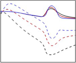
We now investigate the effect of Prandtl number on the eigenspectrum by examining the variation of phase speed and growth rate for the fast and slow modes (Fedorov & Tumin Reference Fedorov and Tumin2011). The phase speed and growth rate variation for different  $Pr$ at $M=4$ are shown in figure 5. In the limit of $\alpha \to 0$, the fast and slow modes are synchronized with the acoustic wave ( $c_{a\pm }=1\pm 1/M$). The phase speed of the fast mode decreases with increasing wavenumber and synchronizes with the continuous spectrum branch corresponding to entropy and vorticity modes ( $C_r=1$). The fast mode after synchronization with the vorticity/entropy modes is termed the mode $F_+$ (Fedorov & Tumin Reference Fedorov and Tumin2011). The phase speed of the fast mode decreases further and it synchronizes with the slow mode. Due to this synchronization the growth rates of the fast and slow modes exhibit a peak and trough (Fedorov & Tumin Reference Fedorov and Tumin2011). The phase speed evolution for the fast and slow modes shown in figure 5(a) are similar for all three Prandtl numbers considered. The synchronization point between the fast and entropy/vorticity mode and the location of discrete spectrum branching is weakly dependent on Prandtl number. At $M=4$, the slow mode is unstable at low wavenumbers while the fast mode ( $F_+$) becomes unstable at high $\alpha$ for all three Prandtl numbers considered. Figure 6 plots the phase speed and growth rates for fast and slow modes at $M=6$. Similar to the case at $M=4$, the phase speed evolution and the synchronization wavenumbers do not have a strong dependence on Prandtl number for $M=6$ as well. However, the branching pattern of the eigenspectrum is dependent on Prandtl number. For low Prandtl number, the mode $F_+$ becomes unstable at high wavenumbers and exhibits a strong peak. On the other hand, for $Pr\geq 0.7$, the slow mode after synchronization with the fast mode becomes the dominant instability. Fedorov & Tumin (Reference Fedorov and Tumin2011) and Ramachandran et al. (Reference Ramachandran, Saikia, Sinha and Govindarajan2015) also report a similar branching pattern of the eigenspectrum depending on the Mach and Prandtl numbers. The effect of Prandtl number on the eigenfunctions of the fast and slow modes at $M=6$, $\alpha =0.05$ is shown in figure 7. The eigenfunctions are normalized by the magnitude of the pressure perturbation at the wall. In the low wavenumber limit, the eigenfunctions of velocity and pressure for both the fast and slow modes do not have a strong dependence on Prandtl number. The eigenfunctions of temperature for the slow mode peak near the critical layer. The critical layer ( $y_{cl}$) is the location in the flow where the phase speed of the instability ( $C_r$) equals the base velocity (Mack Reference Mack1984). In general, $y_{cl}$ increases with Prandtl number, as a result, there is a moderate shift in the location of peak temperature at high Prandtl number. The peak value of the temperature eigenfunction is also larger at $Pr=0.9$ compared with $Pr=0.5$. The eigenfunctions of the fast ( $F_+$) and slow ( $S$) modes before the branching of the discrete spectrum are presented in figure 8. Before the branching of the discrete spectrum the fast mode is more unstable at $Pr=0.5$ (figure 6) while the slow mode is the dominant instability at $Pr=0.9$. The eigenfunctions for the fast and slow modes at both Prandtl numbers are similar before the synchronization point. Figure 9 displays the eigenfunctions of the fast and slow modes near the peak/trough in growth rates. The pressure eigenfunctions for both $F_+$ and $S$ modes are reasonably invariant with $Pr$. The temperature eigenfunction for the $F_+$ mode exhibits a stronger peak at $Pr=0.9$, while the slow mode has higher peak temperature at $Pr=0.5$. This can be attributed to the different branching patterns observed for $Pr=0.5$ and $Pr=0.9$.

Figure 5. Variation of (a) phase speed and (b) growth rate for fast and slow modes with wavenumber at  $M=4$, $Re=4000$ for three different $Pr$. Solid lines correspond to fast mode and dashed lines represent slow mode; (a) $C_r$ and (b) $C_i$.

Figure 6. Variation of (a) phase speed and (b) growth rate for fast and slow modes with wavenumber at  $M=6$, $Re=4000$ for three different $Pr$. Solid lines correspond to fast mode and dashed lines represent slow mode; (a) $C_r$ and (b) $C_i$.

Figure 7. Eigenmode shapes of the (a–c) fast ( $F$) and (d–f) slow ( $S$) modes at $M=6$, $Re=4000$, $\alpha =0.05$, $\beta =0$ for two different Prandtl numbers; (a) $\hat {u}_1$, (b) $\hat {T}$, (c) $\hat {p}$, (d) $\hat {u}_1$, (e) $\hat {T}$ and ( f) $\hat {p}$.

Figure 8. Eigenmode shapes of the (a–c) fast ( $F_+$) and (d–f) slow ( $S$) modes before the branch point at $M=6$, $Re=4000$, $\alpha =0.15$, $\beta =0$ for two different Prandtl numbers; (a) $\hat {u}_1$, (b) $\hat {T}$, (c) $\hat {p}$, (d) $\hat {u}_1$, (e) $\hat {T}$ and ( f) $\hat {p}$.

Figure 9. Eigenmode shapes of the (a–c) fast ( $F_+$) and (d–f) slow ( $S$) modes near peak/trough in growth rate at $M=6$, $Re=4000$, $\alpha =0.175$, $\beta =0$ for two different Prandtl numbers; (a) $\hat {u}_1$, (b) $\hat {T}$, (c) $\hat {p}$, (d) $\hat {u}_1$, (e) $\hat {T}$ and ( f) $\hat {p}$.
5. Prandtl number effects on flow–thermodynamics interactions
The effect of Prandtl number on the flow–thermodynamics interactions is investigated in this section. For simplicity, we only consider the most unstable first/second mode for a given  $(Re,Pr,M)$ combination. The most unstable mode is obtained by sweeping over a range of thestreamwise–spanwise wavenumber pairs ( $\alpha, \beta$). The Reynolds number for all the cases considered here is maintained at $Re=4000$. At each Prandtl number, the most unstable first mode is obtained for $M=\{0.5,1,2,3,4,6\}$, while the most unstable second mode is computed for $M=\{4,5,6,7,8\}$.
We first analyse the effect of Mach number and Prandtl number on the instability growth rate. The growth rates for the most unstable first and second modes are shown in figure 10. The mean growth rates obtained from GKM–DNS for cases  $C1$–
$C1$– $C6$ outlined in table 2 are also plotted in figure 10. The growth rates predicted by GKM–DNS are in excellent agreement with linear analysis for both first and second mode cases. A more rigorous validation by comparing the mode shapes of perturbations for cases $C_{3}$ and $C_{6}$ is provided in Appendix B.

Figure 10. Growth rates for the most unstable (a) first mode and (b) second mode. Filled symbols are from LSA computations and unfilled symbols correspond to results of GKM–DNS cases outlined in table 2. (a) First mode and (b) second mode.
The most unstable first mode is streamwise for the subsonic Mach numbers, and oblique for the supersonic and hypersonic Mach numbers. The obliqueness angle for the most unstable mode decreases with Prandtl number at a given Mach number. At  $Pr=0.5$, the growth rate for the first mode decreases monotonically with Mach number. The high Mach number ( $M\geq 2$) cases are destabilized with increasing Prandtl number while the low Mach number cases are unaffected by Prandtl number changes. The instability growth rates at high Mach numbers increases tenfold as the Prandtl number is increased from $0.5$ to $1.3$. This is consistent with the findings of Ramachandran et al. (Reference Ramachandran, Saikia, Sinha and Govindarajan2015), wherein a similar destabilization of the streamwise first mode is observed for $M=4$.
The most unstable second mode is always aligned along the streamwise direction as the relative supersonic region is of maximum extent for 2-D waves (Mack Reference Mack1984). Much like the first mode, the second mode is also destabilized with increasing Prandtl number, although the destabilization is not as strong as the first mode. As shown in figure 10(b), the growth rate for all Mach numbers considered at  $Pr=1.3$ is more than double the growth rate at $Pr=0.5$. A similar destabilization of the second mode was also observed by Ramachandran et al. (Reference Ramachandran, Saikia, Sinha and Govindarajan2015). The main novelty of the present work is to examine the physics underlying the destabilization with increasing Prandtl number.
5.1. Flow–thermodynamics interactions for the first mode
The influence of Prandtl number on the growth rate can be best understood by examining the flow–thermodynamics interactions in the flow. Toward this end, the internal-kinetic energy exchange for the first mode instability is analysed. For this analysis we define the global average  $Q^g$ as
 \begin{equation} Q^g=\frac{1}{L_{x2}}\int_0^{L_{x2}}\langle Q(x_1,x_2,x_3) \rangle \, {\rm d} x_2. \end{equation}
The global averaged perturbation internal energy is obtained from LSA by integrating the amplitude of pressure perturbations in the wall-normal direction
 \begin{equation} e^g = \frac{1}{L_{x2}}\int_0^{L_{x2}}\frac{\hat{p}(x_2) \hat{p}^c(x_2)}{2\gamma\bar{P}} \, {\rm d} x_2, \end{equation}
where  $\hat {p}$ is the mode shape of pressure perturbation obtained from linear theory and $\hat {p}^c$ is the complex conjugate of $\hat {p}$. Similarly, the global averaged perturbation kinetic energy $k^g$ is determined by the following expression:
 \begin{equation} k^g = \frac{1}{2L_{x2}}\int_0^{L_{x2}}\bar{\rho}(x_2) [\hat{u}_1(x_2)\hat{u}_1^c(x_2)+\hat{u}_2(x_2)\hat{u}_2^c(x_2) +\hat{u}_3(x_2)\hat{u}_3^c(x_2)]\, {\rm d} x_2. \end{equation}
The global averaged perturbation internal energy normalized by the global averaged perturbation kinetic energy at different  $M$ and $Pr$ is presented in figure 11(a). It is evident from figure 11(a) that the internal energy content increases with increasing Prandtl number at high Mach numbers, suggesting thermodynamic effects are stronger in high Prandtl number fluids. For the first mode, the perturbation internal energy content is at least 20 times smaller than the kinetic energy. As mentioned previously, the internal and kinetic modes are coupled via pressure dilatation. The perturbation velocity field interacts with the mean flow and the perturbation internal field via production and pressure dilatation, respectively. Therefore, the ratio of pressure dilatation to production is key for quantifying internal-kinetic energy exchange. The ratio of globally averaged pressure dilatation to production is shown in figure 11(b). The ratio is always negative, indicating energy is transferred from kinetic to the internal mode. The plots also indicate that production is an order of magnitude greater than pressure dilatation for all cases. As pressure dilatation is small compared with production, the internal-kinetic energy exchange is not significant for the first mode.

Figure 11. Global averaged (a) internal energy fraction ( $e^g/k^g$) and (b) pressure-dilatation to production ratio for the most unstable first mode. The symbols are the same as figure 10; (a) $e^g$ and (b) $\varPi _k^g/P_k^g$.
The globally averaged internal energy and pressure-dilatation to production ratio obtained from GKM–DNS are also shown in figure 11(a,b). As the DNSs are initialized by the mode computed from LSA, the mean values of  $e^g$ and $\varPi _k^g/P_k^g$ in time are presented. The spatial derivatives in the $\varPi _k^g$ computations are obtained with spectral accuracy in the homogeneous directions while a fourth-order central difference scheme is employed in the wall-normal direction. The mean $e^g$ and pressure-dilatation to production ratio obtained from GKM–DNS are in good agreement with linear analysis.
We now consider the effect of Prandtl number on the various processes in the kinetic energy budget detailed in (2.16). Once again, the statistics are averaged in the wall-normal direction. The global averaged terms in the kinetic energy budget are normalized by  $\zeta =2k^g U_\infty /L_r$. The normalization ensures that the same level of perturbation kinetic energy is maintained allowing for a valid comparison across different cases. The global average of the transport term is identically zero as the velocity perturbations vanish at the top and bottom boundaries. Figure 12 plots global averaged production ( $P_k^g$), pressure dilatation ( $\varPi _k^g$) and dissipation ( $\epsilon _k^g$) for the first mode at three different Prandtl numbers. At all $Pr$–
$Pr$– $M$ combinations, production is the dominant process and pressure dilatation is considerably smaller. The kinetic energy budget is essentially a balance between production and dissipation. At $Pr=0.5$, production is highest for $M=0.5$ and decreases monotonically with Mach number. Dissipation is fairly constant across all $M$ at this Prandtl number. The production decrease leads to stabilization of the first mode with Mach number at $Pr=0.5$. As the Prandtl number is increased, production increases almost tenfold for the high Mach number cases. On the other hand, production levels are unchanged for the low Mach number ( $M\leq 1$) cases. Dissipation exhibits only a marginal increase with Prandtl number. Thus, the main cause of increased destabilization with $Pr$ is the enhancement of production.

Figure 12. Global averaged terms in the kinetic energy budget: (a) production  $P_k^g$, (b) pressure dilatation $\varPi _k^g$ and (c) dissipation $\epsilon _k^g$ for the most unstable first mode. All budget terms are normalized by $\zeta =2k^g U_\infty /L_r$.
Delving further, we examine the inter-component exchange of energy amongst the three kinetic modes by considering the diagonal components of the stress budget (2.20). The globally averaged terms on the right-hand side of the streamwise component of the stress ( $R_{11}^g$) budget are shown in figure 13(a–c). Since the base flow is two-dimensional and parallel, the streamwise energy production ( $P_{11}^g$) is the only non-zero diagonal component of the production tensor. Consequently, $P_{11}^g$ is equal to twice the total production of kinetic energy. The streamwise component of pressure–strain correlation ( $\varPi _{11}^g$) is of the order of $P_{11}^g$ even though pressure dilatation is negligible. It is evident form figure 13(b) that the sign of $\varPi _{11}^g$ is always negative, indicating that energy is extracted from the streamwise mode. The amount of energy extracted by pressure–strain correlation from the streamwise mode increases with Prandtl number. The streamwise component of the dissipation tensor ( $\epsilon _{11}^g$) is fairly constant with Prandtl number and is the least significant of the three processes. Overall, $P_{11}^g+\varPi _{11}^g$ increases with Pr for a given Mach number.

Figure 13. Global averaged terms in the streamwise kinetic energy ( $R_{11}$) budget: (a) production $P_{11}^g$, (b) pressure–strain correlation $\varPi _{11}^g$ and (c) dissipation $\epsilon _{11}^g$ for the most unstable first mode. All budget terms are normalized by $\zeta =2k^g U_\infty /L_r$.
The averaged terms on the right-hand side of the wall-normal kinetic energy budget are shown in figure 14(a,b). Here,  $P_{22}^g$ is identically zero due to the absence of mean velocity in the wall-normal direction. Energy extracted from the streamwise mode is transferred to the wall-normal mode via $\varPi _{22}^g$. The wall-normal component of the dissipation tensor is negligible, indicating that almost all of the energy transferred to the wall-normal mode is retained. Also, $\varPi _{22}^g$ increases with Prandtl number, resulting in higher kinetic energy in the wall-normal direction. This is shown in figure 14(c), wherein the wall-normal kinetic energy fraction is plotted. The wall-normal kinetic energy content ( $R_{22}^g$) increases with Prandtl number due to increase in $\varPi _{22}^g$. The fraction of wall-normal kinetic energy as obtained from GKM–DNS is also presented in figure 14(c). The results from DNS are in excellent agreement with linear analysis.

Figure 14. Global averaged terms in the wall-normal kinetic energy ( $R_{22}$) budget: (a) pressure–strain correlation $\varPi _{22}^g$ and (b) dissipation $\epsilon _{22}^g$ for the most unstable first mode. (c) Wall-normal kinetic energy fraction ( $R_{22}^g/2k^g$) for the most unstable first mode. All budget terms are normalized by $\zeta =2k^g U_\infty /L_r$. The symbols are the same as figure 10.
Figures 15(a) and 15(b) present the global averaged terms on the right-hand side of the spanwise kinetic energy budget. As the most unstable first mode at  $M=0.5$ is aligned in the streamwise direction, the spanwise kinetic energy is negligible. For the oblique modes ( $M\geq 1$), $\varPi _{33}^g$ provides a source of spanwise energy. Some of this energy is dissipated via the spanwise component of the dissipation tensor $\epsilon _{33}^g$. The dissipated energy is not significant compared with $\varPi _{33}^g$ at high Prandtl numbers. Also, $\varPi _{33}^g$ increases with Prandtl number, resulting in increased energy in the spanwise mode, as shown in figure 15(c). The DNS results for the spanwise energy fraction are also shown in figure 15(c), and once again the agreement with linear analysis is very good.

Figure 15. Global averaged terms in the spanwise kinetic energy ( $R_{33}$) budget: (a) pressure–strain correlation $\varPi _{33}^g$ and (b) dissipation $\epsilon _{33}^g$ for the most unstable first mode. (c) Spanwise kinetic energy fraction ( $R_{33}^g/2k^g$) for the most unstable first mode. All budget terms are normalized by $\zeta =2k^g U_\infty /L_r$. The symbols are the same as figure 10.
The above results indicate that the destabilization of the first mode with Prandtl number is due to increased production. For a parallel flow, production is dependent on the shear stress anisotropy  $\langle R_{12} \rangle$. The shear stress budget is examined in figure 16(a–c). The shear stress production ( $P_{12}$) and the shear component of pressure–strain correlation tensor ( $\varPi _{12}$) are given by the following relation:
 \begin{equation} P_{12} ={-}\langle\bar{\rho}u_2'u_2'\rangle\frac{{\rm d} \bar{U}_1}{{\rm d} x_2}; \quad \varPi_{12} =\left\langle p'\left(\frac{\partial u_1'}{\partial x_2}+ \frac{\partial u_2'}{\partial x_1}\right)\right\rangle. \end{equation}
Here,  $P_{12}$ is dependent on the wall-normal kinetic energy and the mean velocity gradient. As mentioned previously, the wall-normal energy content increases with Prandtl number. Consequently, the global averaged production of shear stress ( $P_{12}^g$) increases in magnitude, as shown in figure 16(a). The absolute value of the ratio $\varPi _{12}^g/P_{12}^g$ is presented in figure 16(b). Here, $\varPi _{12}^g$ is positive for all $(M,Pr)$ combinations. The ratio $|\varPi _{12}^g/P_{12}^g|$ is approximately unity at low Mach numbers and decreases monotonically with increasing Mach number. Furthermore, as the Prandtl number is increased, the ratio $|\varPi _{12}^g/P_{12}^g|$ decreases. It must be noted that $\varPi _{12}^g$ increases with Prandtl number in such a way that the ratio of pressure–strain correlation to shear production decreases. This results in a net increase in the magnitude of the shear stress budget (figure 16c).

Figure 16. (a) Global averaged shear stress production  $P_{12}^g$, (b) absolute value of ratio of pressure–strain correlation $\varPi _{12}^g$ to shear stress production for the most unstable first mode. (c) Sum of all the terms on the right-hand side of the shear stress budget equation (2.20). All budget terms are normalized by $\zeta =2k^g U_\infty /L_r$; (a) $P_{12}^g$, (b) $|\varPi _{12}^g/P_{12}^g|$ and (c) $\varPi _{12}^g+P_{12}^g+\epsilon _{12}^g$.
Seeking the reason for increased production with  $Pr$, we now examine shear stress and mean velocity gradients. The shear stress is shown in figure 17(a). The shear stress becomes more negative with increasing Prandtl number. This is also confirmed by DNS results presented in figure 17(a). The base velocity gradient at the critical layer in the flow is presented in figure 17(b). The location of the critical layer corresponds to maximum production in the flow. Although the base velocity gradient at the critical layer decreases slightly with Prandtl number, the significant increase in the shear stress anisotropy allows for higher production. At $Pr=1.3$, the magnitude of shear stress anisotropy increases monotonically with Mach number. The mean velocity gradient, on the other hand, decreases monotonically with the Mach number. The competing trends for shear stress anisotropy and mean velocity gradient leads to a production peak (figure 12) at $M=4$ for $Pr=1.3$.

Figure 17. (a) Shear stress anisotropy ( $R_{12}^g/2k^g$) for the most unstable first mode. (b) Mean velocity gradient ( $\textrm {d} \bar {U}_1/\textrm {d} x_2$) at the critical layer for the most unstable first mode. The symbols are the same as figure 10.
5.2. Flow–thermodynamics interactions for the second mode
In this subsection, we analyse the effect of Prandtl number on the flow–thermodynamics interaction of the most unstable second mode. The global averaged perturbation internal energy normalized by  $k^g$ for the most unstable second mode is shown in figure 18(a). The internal energy content increases with Prandtl number as thermodynamic effects become stronger with increasing Prandtl number. Unlike the first mode, internal energy for the second mode is of the same order as the perturbation kinetic energy. The internal-kinetic energy interactions can be quantified by the ratio of pressure dilatation to production shown in figure 18(b). The ratio $\varPi _k^g/P_k^g\sim O(1)$, indicating pressure work is significant for the second mode. Energy is transferred from the kinetic to the internal mode as $\varPi _k^g/P_k^g$ is always negative. For a given Mach number, the ratio of pressure dilatation to production decreases in magnitude with Prandtl number, and yet the internal energy fraction increases with Prandtl number. The mean values of $e^g$ and $\varPi _k^g/P_k^g$ computed from GKM–DNS also shown in figure 18(a,b) are in excellent agreement with linear analysis.

Figure 18. Global averaged (a) internal energy fraction ( $e^g/k^g$) and (b) pressure-dilatation to production ratio for the most unstable second mode. The symbols are the same as figure 10; (a) $e^g$ and (b) $\varPi _k^g/P_k^g$.
We now analyse the effect of Prandtl number on the flow processes. The global average of the terms on the right-hand side of the kinetic energy budget (2.16) are shown in figure 19(a–c). As in the case of the first mode, production is the dominant process and increases with Prandtl number. Dissipation also increases with Prandtl number, although it is small compared with production at high Prandtl numbers. Pressure dilatation for the second mode is non-negligible, as seen previously. This kinetic to internal energy transfer becomes stronger as the Prandtl number of the fluid increases. Nonetheless, the increase in  $P_k^g$ is larger compared with the other two processes, resulting in higher kinetic energy growth rates with increasing Prandtl number.

Figure 19. Global averaged terms in the kinetic energy budget: (a) production  $P_k^g$, (b) pressure dilatation $\varPi _k^g$ and (c) dissipation $\epsilon _k^g$ for the most unstable second mode. All terms in the budget are normalized by $\zeta =2k^g U_\infty /L_r$.
The inter-component energy transfer amongst the normal stresses is considered next. Since the most unstable second mode is always aligned with the streamwise direction, the spanwise modes have no energy. Figures 20(a)–20(c) plot the global averaged production of the streamwise kinetic energy ( $P_{11}^g$), the streamwise pressure–strain correlation ( $\varPi _{11}^g$) and the streamwise component of the dissipation tensor ( $\epsilon _{11}^g$), respectively. Similar to the first mode, $P_{11}^g$ equals twice the total production of kinetic energy. Pressure–strain correlation extracts energy from the streamwise mode. The amount of energy extracted increases with Prandtl number. A small portion of the energy gained via production is dissipated, and the effect of dissipation increases slightly with Prandtl number.

Figure 20. Global averaged terms in the streamwise kinetic energy ( $R_{11}$) budget: (a) production $P_{11}^g$, (b) pressure–strain correlation $\varPi _{11}^g$ and (c) dissipation $\epsilon _{11}^g$ for the most unstable second mode. All terms in the budget are normalized by $\zeta =2k^g U_\infty /L_r$.
Once again,  $\varPi _{22}^g$ provides a source of wall-normal energy. This is evident from figure 21(a,b), wherein the global averaged terms of the wall-normal kinetic energy budget are shown. A small fraction of the energy attained by $\varPi _{22}^g$ is dissipated by the wall-normal perturbations via $\epsilon _{22}$. Also, $\varPi _{22}^g$ increases with Prandtl number whereas $\epsilon _{22}^g$ is fairly constant across all Prandtl numbers. The higher pressure–strain correlation level leads to increased energy content in the wall-normal mode with increasing Prandtl number. This is shown in figure 21(c), wherein the fraction of wall-normal energy is presented. The DNS results are also presented in the same figure, corroborating the linear analysis findings.

Figure 21. Global averaged terms in the wall-normal kinetic energy ( $R_{22}$) budget: (a) pressure–strain correlation $\varPi _{22}^g$ and (b) dissipation $\epsilon _{22}^g$ for the most unstable second mode. (c) Wall-normal kinetic energy fraction ( $R_{22}^g/2k^g$) for the most unstable second mode. All budget terms are normalized by $\zeta =2k^g U_\infty /L_r$. The symbols are the same as figure 10.
The wall-normal component of kinetic energy contributes to the production of shear stress ( $R_{12}$). The shear stress budget is examined in figure 22(a–c). Unlike the first mode, the shear stress production ( $P_{12}^g$) decreases in magnitude with Prandtl number. The absolute value of the ratio of $\varPi _{12}^g$ to $P_{12}^g$ is of the order of unity. This is consistent with the findings of Bertsch, Suman & Girimaji (Reference Bertsch, Suman and Girimaji2012) for homogeneous shear flows. For a given Prandtl number, the ratio decreases monotonically with Mach number. Also, $|\varPi _{12}^g/P_{12}^g|$ decreases with Prandtl number at a given $M$. This results in net magnitude increase of the shear stress budget, as shown in figure 22(c).

Figure 22. Global averaged shear stress production  $P_{12}^g$, (b) absolute value of ratio of pressure–strain correlation $\varPi _{12}^g$ to shear stress production for the most unstable second mode. (c) Sum of all the terms on the right-hand side of the shear stress budget equation (2.20). All budget terms are normalized by $\zeta =2k^g U_\infty /L_r$; (a) $P_{12}^g$, (b) $|\varPi _{12}^g/P_{12}^g|$ and (c) $P_{12}^g+\varPi _{12}^g+\epsilon _{12}^g$.
We now examine the kinetic energy production. Figures 23(a) and 23(b) plot the averaged shear stress anisotropy and the base velocity gradient at peak production, respectively. The maximum production is at the sonic line for low Prandtl number fluids but moves toward the boundary layer edge as the Prandtl number is increased. The sonic line ( $x_{2a}$) is defined as the location in the flow wherein the relative disturbance Mach number ( $M_r$) equals 1. The relative disturbance Mach number (Mack Reference Mack1984) is defined as
 \begin{equation} M_r=\frac{(\alpha \bar{U}_1 -\omega_r)M}{[(\alpha^2+\beta^2)\bar{T}]^{1/2}}. \end{equation}
The magnitude of the globally averaged shear stress anisotropy increases with Prandtl number but the base velocity gradient at peak production decreases with Prandtl number. The significant increase in the shear stress magnitude permits the high levels of production observed in figure 19(a). For a fixed Prandtl number, the magnitude of  $R_{12}^g$ increases with Mach number while the base flow gradient at peak production decreases. This results in a non-monotonic dependence of production with respect to Mach number, as shown in figure 19(a). The mean $R_{12}^g$ obtained from DNS is also shown in figure 23(a). The DNS results are in excellent agreement with linear analysis.

Figure 23. (a) Shear stress anisotropy ( $R_{12}^g/2k^g$) for the most unstable second mode. (b) Mean velocity gradient ( $\textrm {d} \bar {U}_1/ \textrm {d} x_2$) at peak production for the most unstable second mode. The symbols are the same as figure 10.
Finally, we examine the internal energy budget (2.19) in figure 24(a–c). Internal and kinetic modes exchange energy via pressure dilatation. The kinetic to internal energy transfer increases with Prandtl number at a given Mach number. The perturbation internal mode also interacts with the mean internal mode via the thermal flux ( $T_s^g$) and viscous terms ( $\epsilon _s^g$). A significant portion of the energy gained by the perturbation internal mode is transferred to the mean internal mode via the action of thermal flux. The thermal flux action weakens with increasing Prandtl number as it is inversely proportional to Prandtl number. The viscous action is small compared with $\varPi _k^g$ and $T_s^g$. The increased pressure work combined with reduced thermal flux action leads to higher internal energy content in high Prandtl number fluids (figure 18a).

Figure 24. Global averaged terms in the internal energy budget: (a) negative of pressure dilatation  $-\varPi _{k}^g$, (b) thermal flux $T_{s}^g$ and (c) viscous term $\epsilon _s^g$ for the most unstable second mode. All budget terms are normalized by $\zeta =2k^g U_\infty /L_r$.
5.3. Flow physics underlying Prandtl number effects
In this subsection the sequence of flow processes underlying the observed  $Pr$ effects on the first and second modes will be summarized. It is already established that for both the first and second modes the averaged shear stress anisotropy increases with Prandtl number. And yet, $P_{12}^g$ increases with Prandtl number for first mode while it decreases for the second mode. We examine the contrasting behaviour of $P_{12}^g$ by considering the profiles of wall-normal kinetic energy ( $R_{22}$), base flow gradient ( $\textrm {d} \bar {U}_1/ \textrm {d} x_2$) and $P_{12}$. The profiles for first mode at $M=4$ are shown in figure 25(a–c). For the first mode, the wall-normal kinetic energy increases with Prandtl number throughout the boundary layer. The base flow gradient near the $R_{22}$ peak is also higher at high Prandtl numbers. Therefore, $P_{12}^g$ increases with Prandtl number for the first mode.

Figure 25. Profiles of (a) wall-normal kinetic energy ( $R_{22}$), (b) mean velocity gradient $\textrm {d} \bar {U}_1/ \textrm {d} x_2$ and (c) production of shear stress ( $P_{12}$) for the most unstable first mode at $M=4$.
We now summarize the flow–thermodynamics interactions for the first mode. A schematic representing the key interactions is displayed in figure 26. Energy is extracted from the mean flow via production and transferred to the streamwise perturbations. Pressure dilatation (pressure work) is not significant and does not play an important role in the instability dynamics. The effect of Prandtl number manifests through pressure–strain correlation. Production and all components of pressure–strain correlation increase with Prandtl number. The more energetic wall-normal mode leads to a rise in the production of shear stress. The ratio of  $P_{12}^g$ to $\varPi _{12}^g$ decreases with Prandtl number. As a result, the difference of $P_{12}^g$ and $\varPi _{12}^g$ increases with Prandtl number, leading to increased magnitude of shear stress anisotropy. The higher shear stress anisotropy ultimately allows for higher production, leading to increased destabilization at higher Prandtl number.

Figure 26. Schematic of energy interactions between internal and kinetic modes for the first mode instability. Up/down arrows indicate increasing/decreasing magnitude of the processes with increasing Prandtl number.
For the second mode, the global averaged wall-normal energy ( $R_{22}^g$) increases with Prandtl number while $P_{12}^g$ decreases in magnitude with Prandtl number. The profiles of $R_{22}$, base flow gradient and $P_{12}$ for the second mode at $M=4$ are shown in figure 27(a–c), respectively. Unlike the case of the first mode, the $R_{22}$ profile has a global and a local maximum. The global maximum is located near the sonic line ( $x_2\approx 3$). The global maximum of the wall-normal energy decreases with Prandtl number. The mean velocity gradient near the sonic line also decreases with Prandtl number. Hence, the low Prandtl number fluid has a much stronger global minimum of $P_{12}$, located near the sonic line. The local $R_{22}$ maximum, near the boundary layer edge ( $x_{2}\approx 10$) is stronger for higher Prandtl number fluid. However, the mean flow gradient is negligible near the boundary layer edge. Consequently, the local $P_{12}$ minimum near the boundary layer edge is substantially smaller compared with the global minimum, leading to a decrease in $P_{12}^g$ magnitude with increasing Prandtl number.

Figure 27. Profiles of (a) wall-normal kinetic energy ( $R_{22}$), (b) mean velocity gradient $\textrm {d} \bar {U}_1/ \textrm {d} x_2$ and (c) production of shear stress ( $P_{12}$) for the most unstable second mode at $M=4$.
The flow–thermodynamics interactions for the second mode are summarized in the schematic shown in figure 28. Energy is transferred from the mean flow to the streamwise mode of perturbation kinetic energy via production. Unlike the first mode, pressure dilatation is significant for the second mode. Pressure work transfers energy from the kinetic to the internal mode and pressure–strain correlation redistributes energy amongst the stress components. Production, pressure dilatation and the diagonal components of  $\varPi _{ij}^g$ increase with Prandtl number. This leads to higher wall-normal and internal energy with increasing Prandtl number. The production of shear stress and the shear component of pressure–strain correlation decrease with Prandtl number. The difference of $P_{12}^g$ and $\varPi _{12}^g$ increases with Prandtl number, leading to high shear stress anisotropy. The increased shear stress anisotropy permits the higher level of production leading to increased instability growth rate at higher Prandtl number.

Figure 28. Schematic of energy interactions between internal and kinetic modes for the second mode instability. Up/down arrows indicate increasing/decreasing magnitude of the processes with increasing Prandtl number.
6. Boundary layer response to random pressure forcing at different Prandtl numbers
The nature and composition of free-stream disturbances is not necessarily known for all transition experiments (Hader & Fasel Reference Hader and Fasel2018). Consequently, Hader & Fasel (Reference Hader and Fasel2018) modelled the free-stream disturbance by random pressure (acoustic) disturbances to simulate natural transition in high speed boundary layers. More recently, Mittal, Sharma & Girimaji (Reference Mittal, Sharma and Girimaji2021) employed random acoustic disturbances to study instability evolution in Poiseuille flow. Following previous works, we perform DNSs of temporally evolving boundary layers with randomly generated pressure forcing at different Mach and Prandtl numbers. The temporal simulations are initialized by a laminar basic state superposed with low intensity random pressure forcing (Hader & Fasel Reference Hader and Fasel2018; Mittal et al. Reference Mittal, Sharma and Girimaji2021). The intensity of pressure forcing is  $1\,\%$ of the free-stream pressure. The simulations are performed at $M=3$ and $M=6$ for $Pr=\{0.5,0.7,1.3\}$. The grid sizes and relevant parameters for the simulations are listed in table 3.
Table 3. Non-dimensional parameters, free-stream properties and grid sizes for DNSs with random pressure forcing.

The evolution of globally averaged kinetic and internal energy at  $M=6$ for three different Prandtl numbers is shown in figure 29. After the lapse of an initial transience, kinetic energy grows exponentially at the dominant eigenmode growth rate predicted by LSA. The dominant eigenmode corresponds to the streamwise–spanwise wavenumber pair $(10,0)$ for $Pr=\{0.5,0.7\}$, while the mode $(12,0)$ dominates for $Pr=1.3$. Here, $(m,n)$ denotes the $m$th and $n$th harmonic of the fundamental streamwise and spanwise wavenumber resolved by the simulation. The asymptotic growth rate of $k^g$ increases with increasing Prandtl number. Since the dominant mode at $M=6$ is a second mode, the internal energy also grows beyond the transient region and the growth rate of $e^g$ agrees well with LSA. The initial forcing generates a broadband spectrum with energy randomly distributed in all wavenumbers. This is evident from the spectral spread of global kinetic energy shown in figure 30. The high wavenumbers are linearly stable and dissipate quickly, resulting in kinetic energy decay in the transient stage. As a result by $t=500$ most of the energy is contained in the linearly unstable wavenumbers. During the transient stage non-modal interactions are prevalent and the evolution cannot be determined by an eigenmode analysis. The length of the transient stage decreases with increasing Prandtl number (figure 29). Consequently, the higher Prandtl number cases attain the asymptotic state faster and are more energetic at all times than the low $Pr$ case. For $Pr=0.5$ the Fourier mode $(10,0)$ becomes the most energetic mode at late times. Linear stability analysis also predicts the mode $(10,0)$ as the fastest growing mode. The kinetic energy spectrum for higher Prandtl number cases has multiple modes with similar energy content. The modes $(10,0)$ and $(10,1)$ are the most energetic modes for $Pr=0.7$. This is perhaps due to the fact that the most unstable eigenmodes corresponding to $(10,0)$ and $(10,1)$ have similar growth rates. Similarly, the modes $(10,0)$, $(11,1)$ and $(12,0)$ are most energetic for $Pr=1.3$. The Fourier mode shapes corresponding to mode $(10,0)$ at late times are presented in figure 31. For all three Prandtl numbers, the mode shapes obtained from DNS are in excellent agreement with the dominant eigenmode shapes obtained from LSA. This confirms that in the asymptotic limit the boundary layer response to external forcing is completely characterized by the most unstable eigenmode(s).

Figure 29. Evolution of globally averaged (a) kinetic energy ( $k^g$) and (b) internal energy ( $e^g$) at $M=6$ and $Re=4000$ for three different Prandtl numbers. The dashed lines represent the dominant eigenmode growth at the rate predicted by LSA; (a) $k^g$ and (b) $e^g$.

Figure 30. Global kinetic energy ( $k^g$) spectrum at $M=6$, $Re=4000$ for (a–c) $Pr=0.5$, (d–f) $Pr=0.7$ and (g–i) $Pr=1.3$.

Figure 31. Mode shapes corresponding to mode  $(10,0)$ at $M=6$, $Re=4000$ for (a–c) $Pr=0.5$, (d–f) $Pr=0.7$ and (g–i) $Pr=1.3$: (a) $\hat{u}_1$, (b) $\hat{T}$, (c) $\hat{p}$, (d) $\hat{u}_1$, (e) $\hat{T}$, (f) $\hat{p}$, (g) $\hat{u}_1$, (h) $\hat{T}$ and (i) $\hat{p}$.
The evolution of globally averaged terms in the kinetic energy budget are shown in figure 32(a–c). Production increases exponentially after the lapse of the transient stage for all  $Pr$. In the transient regime, $P_k^g$ exhibits a oscillatory behaviour and is always positive. The production level increases with Prandtl number at all times. Dissipation decays with time initially and grows exponentially once the transient stage ends. Much like production, dissipation is higher at high Prandtl numbers for all times. The evolution of pressure-dilatation magnitude shown in figure 32(b) suggests that $\varPi _k^g$ also has an exponential variation in the asymptotic limit. At late times, pressure dilatation is negative as energy is transferred from the kinetic to internal mode. However, in the transient stage, $\varPi _k^g$ is dominantly positive as energy is transferred from the internal to the kinetic mode. This is not surprising as, initially, all the perturbation energy is in the internal mode and pressure does work on the velocity field to facilitate the energy transfer. Similar to $P_k^g$ and $\epsilon _k^g$, at late times the magnitude of $\varPi _k^g$ is also higher for high Prandtl number. During the transient stages, however, pressure dilatation is similar in magnitude for all three Prandtl numbers. Figure 33 presents the kinetic energy budget terms normalized by the instantaneous kinetic energy at $M=6$. The normalization ensures that the budget term asymptotes to a constant at late times. The asymptotic value is approximately equal to the budget contributions of the most unstable eigenmode predicted by linear theory. This is also not surprising, as at late times, the evolution is determined by the most unstable eigenmode.

Figure 32. Evolution of globally averaged terms in the kinetic energy budget: (a) production ( $P_k^g$), (b) absolute value of pressure dilatation ( $|\varPi _k^g|$) and (c) dissipation ( $-\epsilon _k^g$) at $M=6$ and $Re=4000$ for three different Prandtl numbers. The dashed lines represent dominant eigenmode growth at the rate predicted by LSA.

Figure 33. Evolution of globally averaged terms in the kinetic energy budget normalized by instantaneous kinetic energy for (a)  $Pr=0.5$, (b) $Pr=0.7$ and (c) $Pr=1.3$ at $M=6$ and $Re=4000$. All budget terms are normalized by $\zeta =2k^g U_\infty /L_r$. The dashed lines represent the budget contributions of the most unstable eigenmode predicted by LSA.
The kinetic energy evolution at  $M=3$ and $Re=4000$ for different $Pr$ is shown in figure 34. Similar to the $M=6$ case, $k^g$ at $M=3$ also increases exponentially after a transient decay stage. The length of the transient stage also decreases with increasing $Pr$. The kinetic energy growth at late times is slower than the most unstable eigenmode growth rate predicted by LSA. At $M=3$ for all Prandtl numbers, there exist several modes with growth rates nearly identical to the most unstable mode. As a result, there are multiple Fourier modes with similar energy content at late times. However, the mode shapes for these modes are qualitatively similar. The kinetic energy budget terms normalized by instantaneous kinetic energy is presented in figure 35. The budget terms at $M=3$ also asymptote to the contributions of the most unstable eigenmode.

Figure 34. Evolution of globally averaged kinetic energy ( $k^g$) at $M=3$ and $Re=4000$ for three different Prandtl numbers. The dashed lines represent the dominant eigenmode growth at the rate predicted by LSA.

Figure 35. Evolution of globally averaged terms in the kinetic energy budget normalized by instantaneous kinetic energy for (a)  $Pr=0.5$, (b) $Pr=0.7$ and (c) $Pr=1.3$ at $M=3$ and $Re=4000$. All budget terms are normalized by $\zeta =2k^g U_\infty /L_r$. The dashed lines represent the budget contributions of the most unstable eigenmode predicted by LSA.
Overall, the response of the boundary layer to random pressure forcing can be completely determined by the most unstable eigenmode(s) at late times. Since the growth rate of the most unstable eigenmode increases with  $Pr$, random pressure forcing leads to substantial increase in perturbation energy growth for high Prandtl numbers. There exists a transient region where non-modal interactions are significant. During the transient stage total energy decays as dissipation dominates production. The length of transient regime increases with decreasing $Pr$.
$Pr$.
7. Conclusions
In this work, the influence of the Prandtl number on the flow–thermodynamics interaction for compressible boundary layer instability is examined. LSA and DNS of compressible boundary layers are performed in the parameter regimes  $M\in [0.5,8]$ and $Pr\in [0.5,1.3]$. The most unstable first and second modes are identified and the influence of both Mach and Prandtl numbers is studied. Both first and second modes are destabilized by increasing Prandtl number. The underlying flow–thermodynamics interactions are investigated. It is shown that the internal energy content is negligible compared with kinetic energy for the first mode, while the second mode has considerable internal energy content. Pressure dilatation is not significant for the first mode and does not play an important role in the instability dynamics. For the second mode, pressure work transfers considerable energy from the perturbation kinetic to the internal mode.
Despite the marked difference in pressure dilatation both modes exhibit increased production with Prandtl number. In the case of the first mode all components of the pressure–strain correlation increase with Prandtl number. Higher energy in the wall-normal mode leads to increased production of the shear stress at high Prandtl number. The shear pressure–strain correlation also increases with Prandtl number but not as rapidly as shear production. Thus, the net difference between  $P_{12}^g$ and $\varPi _{12}^g$ increases with Prandtl number. The net shear stress anisotropy increase permits higher production leading to increased destabilization of the first mode at higher Prandtl numbers. In the case of the second mode, both $P_{12}^g$ and $\varPi _{12}^g$ decrease with Prandtl number. However, the net difference of $P_{12}^g$ and $\varPi _{12}^g$ increases with Prandtl number. The resulting higher shear stress anisotropy allows for increased production levels at higher Prandtl numbers leading to increased growth rates at high Prandtl numbers. These findings not only enhance our understanding of Prandtl number effects, they also provide the insight needed for closure model development.
Acknowledgements
Portions of this research were conducted with the advanced computing resources provided by Texas A&M High Performance Research Computing.
Declaration of interests
The authors report no conflict of interest.
Appendix A
A.1. Linearized perturbation equations
The linearized perturbation equations (Malik Reference Malik1989) for a compressible parallel boundary layer flow are detailed in this subsection. The linearized continuity equation is given by the following relation:
 \begin{equation} \frac{\partial \rho'}{\partial t} + \bar{U}_i\frac{\partial \rho'}{\partial x_i} +\frac{\partial \bar{\rho}}{\partial x_i}u_i' + \bar{\rho}\frac{\partial u_i'}{\partial x_i} = 0. \end{equation}
The momentum equations are obtained as
 \begin{equation} \bar{\rho}\frac{\partial u_i'}{\partial t} + \bar{\rho}\bar{U}_k\frac{\partial u_i'}{\partial x_k} +\bar{\rho}\frac{\partial \bar{U}_i}{\partial x_k}u_k' ={-}\frac{\partial p'}{\partial x_i} +\frac{1}{Re}\frac{\partial {\mathsf \tau}_{ik}'}{\partial x_k},\end{equation}
where  ${\mathsf \tau} _{ik}'$ is the linearized viscous stress tensor. The components of the linearized viscous stress tensor ${\mathsf \tau} _{ik}'$ are given by
 \begin{equation} {\mathsf \tau}_{ik}'=\bar{\mu}\left(\frac{\partial u_i'}{\partial x_k}+\frac{\partial u_k'}{\partial x_i}\right)+\mu'\left(\frac{\partial \bar{U}_i}{\partial x_k}+\frac{\partial \bar{U}_k}{\partial x_i}\right)+\bar{\lambda}\frac{\partial u_k'}{\partial x_k}\delta_{ik}. \end{equation}
Here,  $\bar {\lambda }$ is the bulk viscosity and is set to $\bar {\lambda }=-2\bar {\mu }/3$.
The energy equation can be expressed in multiple formulations. In the present work, the energy equations in both the enthalpy and pressure formulations are utilized. The energy equation expressed in the enthalpy formulation is employed for linear stability computations whereas the pressure formulation is used to describe the flow–thermodynamics interactions. The linearized energy equation in the enthalpy formulation is expressed as
 \begin{align} \bar{\rho}\frac{\partial T'}{\partial t} + \bar{\rho}\bar{U}_i\frac{\partial T'}{\partial x_i} + \bar{\rho}u_i'\frac{\partial \bar{T}}{\partial x_i} &= (\gamma-1)M^2\left[\frac{\partial p'}{\partial t}+\bar{U}_i\frac{\partial p'}{\partial x_i}\right] - \frac{1}{RePr}\frac{\partial q_k'}{\partial x_k} \nonumber\\ & \quad + \frac{(\gamma-1)M^2}{Re}\left[\tau_{ij}'\frac{\partial \bar{U}_i}{\partial x_j} + \bar{{\mathsf \tau}}_{ij}\frac{\partial u_i'}{\partial x_j}\right]. \end{align}
Here,  $q_k'$ is the perturbation thermal conductivity as defined below
 \begin{equation} q_k'={-}\bar{\kappa}\frac{\partial T'}{\partial x_k}-\kappa'\frac{{\rm d} \bar{T}}{{\rm d} x_k}. \end{equation}
The energy equation expressed in the pressure formulation is given by the following relation:
 \begin{equation} \frac{\partial p'}{\partial t} + \bar{U}_i\frac{\partial p'}{\partial x_i} ={-}\gamma\bar{P} \frac{\partial u_k'}{\partial x_k} - \frac{1}{RePrM^2}\frac{\partial q_k'}{\partial x_k} + \frac{\gamma-1}{Re}\left[\tau_{ij}'\frac{\partial \bar{U}_i}{\partial x_j} + \bar{{\mathsf \tau}}_{ij}\frac{\partial u_i'}{\partial x_j}\right]. \end{equation}
The density perturbations are related to pressure and temperature perturbations by the following state equation:
 \begin{equation} \rho'=\gamma M^2\frac{p'}{\bar{T}}-\frac{\bar{\rho}}{\bar{T}}T'. \end{equation}
A.2. Components of matrices  $A$ and $B$


The components of the coefficient matrices  $\boldsymbol {A}$ and $\boldsymbol {B}$ in (2.12) are detailed in this appendix. It must be noted that the components of the coefficient matrices for the same eigenvalue problem expressed in a marginally different form are presented in Appendix I of Malik (Reference Malik1990). For the sake of clarification, the components of the coefficient matrices are presented here as well. The non-zero elements of matrix $\boldsymbol {A}$ are as follows:
 \begin{equation} \left.\begin{array}{c@{}} \displaystyle A_{11}={-}1;\quad A_{22}={-}1;\quad A_{33}={-}1;\quad A_{44}= \dfrac{1}{\bar{T}}; \\ A_{45}={-}\gamma M^2;\quad A_{54}={-} 1;\quad A_{55}= (\gamma-1)M^2\bar{T}. \end{array}\right\} \end{equation}
The elements of matrix  $\boldsymbol {B}$ are listed below

Here, the symbols  $D$ and $D^2$ denote the first- and second-order derivatives in the wall-normal direction, respectively.
Appendix B. Validation of GKM–DNS
The DNS results are validated by comparing against LSA. The evolution for volume averaged perturbation kinetic energy  $k$ is shown in figure 36 for cases $C_3$ and $C_6$. The kinetic energy is normalized by the initial perturbation kinetic energy. For both cases, the kinetic energy grows exponentially. The growth rate of kinetic energy agrees very well with the rate predicted by linear stability analysis.

Figure 36. Evolution of globally averaged kinetic energy ( $k^g$) for (a) case $C_3$ and (b) case $C_6$. Solid black line corresponds to DNS results and kinetic energy growth based on LSA is marked with red symbols.
The mode shape profiles for the case  $C_3$ at $t=1446$ and $t=0$ are shown in figure 37. Specifically, the mode shapes for streamwise velocity, wall-normal velocity, temperature and density are presented. The mode shapes are initialized with the profiles based on LSA. The mode shape profiles of all the disturbances are retained throughout the duration of the simulation. A similar plot of the mode shapes for the case $C_6$ is displayed in figure 38. The mode shapes for the second mode case are also retained throughout the simulation. Overall, the GKM–DNS results are in excellent agreement with LSA results.

Figure 37. Mode shapes of (a) streamwise velocity, (b) wall-normal velocity, (c) temperature and (d) density for case  $C_3$ at two different times; (a) $\hat {u}_1$, (b) $\hat {u}_2$, (c) $\hat {T}$ and (d) $\hat {\rho }$.

Figure 38. Mode shapes of (a) streamwise velocity, (b) wall-normal velocity, (c) temperature and (d) density for case  $C_6$ at two different times; (a) $\hat {u}_1$, (b) $\hat {u}_2$, (c) $\hat {T}$ and (d) $\hat {\rho }$.


 Open access