


1. Introduction
In density-stratified flows, small-scale turbulence is known to enhance the rate at which density gradients are irreversibly smoothed by diffusive processes (i.e. mixed) and quantifying this rate in geophysical, environmental and industrial settings is of crucial importance. For instance, turbulent mixing is known to have a leading-order impact on global oceanic circulations (Wunsch & Ferrari Reference Wunsch and Ferrari2004). Stratified turbulent flows are characterised by a variety of length scales associated with the structure of the turbulent velocity and density fields. Velocity fluctuations are smoothed by molecular viscosity and dissipated into heat below the Kolmogorov scale  $L_{K} := (\nu ^{3}/\epsilon )^{1/4}$ (where $\nu$ is the molecular viscosity and $\epsilon$ is the appropriately volume-averaged dissipation rate of turbulent kinetic energy). Similarly, density fluctuations are dissipated by molecular diffusion below the Batchelor scale $L_{\rho } := (\nu \kappa ^{2} / \epsilon )^{1/4}$, $\kappa$ being the molecular diffusivity. The (molecular) Prandtl number $Pr := \nu / \kappa$, that effectively quantifies the relative strength of viscous dissipation to diffusion, is the ratio of the square of these two length scales. Unlike the atmosphere, in which $Pr \simeq 0.7$ ( $L_K \approx L_{\rho }$), in the ocean $Pr \sim {O}(10)$ when thermally stratified and the equivalent Schmidt number $Sc:=\nu /D \sim {O}(1000)$ ( $D$ being the salt diffusivity) when dominantly salt-stratified.
For turbulent flows with  $Pr \gg 1$, the inevitable scale separation with $L_\rho \ll L_K$ is such that fully resolved numerical simulations are highly challenging. However, there is increasing evidence indicating that the value of $Pr$ has (perhaps unsurprisingly) a leading-order impact on irreversible scalar-mixing properties of stratified turbulent flows. For instance, the effects of $Pr$ variations on the properties of secondary instabilities arising from the breakdown of Kelvin–Helmholtz billows were reported by Mashayek & Peltier (Reference Mashayek and Peltier2011) and Salehipour, Peltier & Mashayek (Reference Salehipour, Peltier and Mashayek2015). Similarly, Zhou, Taylor & Caulfield (Reference Zhou, Taylor and Caulfield2017) studied the influence of $Pr$ variations on fully developed turbulence in stratified plane Couette flows using direct numerical simulations (DNS) and reported significant effects on density and momentum fluxes. Also using DNS, Legaspi & Waite (Reference Legaspi and Waite2020) analysed the effects of $Pr$ variations on homogeneous forced stratified turbulence and showed, at least for the range of parameters they considered, that the $Pr=1$ simulations are able to describe $Pr > 1$ dynamics at large scales and also that kinetic energy spectra (which importantly do not directly contain information from the density field) are largely unaffected by variations in $Pr$. However, they did observe $Pr$ effects at small scales below $L_K$ and in the density flux spectra. Therefore, here we focus on the influence of $Pr$ variations on small-scale structures of the density field and their associated effects on the mixing properties of forced stratified turbulent flows.
Another important length scale associated with stratified turbulent flows is the buoyancy length scale  $L_{B} := 2{\rm \pi} U / N_{0}$, where $U$ is a characteristic velocity of the flow and $N_{0}$ is a characteristic (background) value of the buoyancy frequency. Scaled using a characteristic horizontal length scale $L_{h}$, this parameter then defines a horizontal Froude number $Fr_{h} := L_{B} / L_{h} = 2{\rm \pi} U / N_{0}L_{h}$ that quantifies the relative strength of the stratification of the flow. For small horizontal Froude numbers $Fr_{h}$ (i.e. relatively strongly stratified flows), the density field is known to self-organise into relatively well-mixed ‘layers’ (whose size scales as $L_{B}$; the buoyancy scale can therefore be thought of as the largest energetically possible overturn) separated by relatively thin ‘interfaces’ of enhanced density gradient (Billant & Chomaz Reference Billant and Chomaz2001; Waite Reference Waite2011). Such density ‘staircase’ structure has important implications for irreversible scalar mixing in density-stratified turbulent flows. Couchman, de Bruyn Kops & Caulfield (Reference Couchman, de Bruyn Kops and Caulfield2023) showed that (in the $Pr=1$ case) while static instabilities are most prevalent within the well-mixed layers (that are hence characterised by relatively high values of $\epsilon$), much of the scalar mixing, as described by the (appropriately volume-averaged) buoyancy variance destruction rate $\chi$, is located in the relatively strongly stratified interfaces, a phenomenon that is not apparent when considering $\epsilon$ only. Hence, we focus here on the contribution of the different structures described above to the overall mixing properties of the flow, as described by $\chi$. Note that we focus in this work on $\chi$ to describe mixing since this microstructure measurement currently provides the best observational means of probing ocean mixing (Gregg et al. Reference Gregg, D'Asaro, Riley and Kunze2018). Other quantities are also used in practical settings, such as buoyancy fluxes or turbulent diffusivities. However, these quantities usually rely upon some kind of averaging or parametrisation and our goal in this work is to probe the small-scale ‘raw’ structures of the density field and their contribution to mixing.
Fundamentally, we aim to understand how the density field's small-scale organisation shapes the bulk mixing properties of forced stratified turbulent flows at different Prandtl numbers. To this end, we analyse fully resolved DNS data of forced stratified turbulent flows at  $Pr=1$ and $Pr=7$, each with $Fr=0.5$ and $Fr=2$, for values of $Re$ such that the emergent $Re_{b}=50$. The rest of this paper is organised as follows. We describe the DNS data in § 2 and then present the methodology used to extract distinct classes of density field structures in § 3. In § 4, we apply this methodology to the DNS data to segment the density field into weakly and strongly stratified interfaces, relatively small-scale ‘lamella-like’ structures and larger-scale density inversions and analyse the associated mixing properties of the extracted density structures. Brief conclusions are drawn in § 5.
2. Summary of the DNS datasets
We consider statistically steady, forced, fully resolved DNS of stratified turbulence from the simulation campaign originally reported by Almalkie & de Bruyn Kops (Reference Almalkie and de Bruyn Kops2012). The non-hydrostatic dimensionless Navier–Stokes equations under the Boussinesq approximation,
 \begin{equation} \left. \begin{gathered} \partial_{t}\boldsymbol{u} + \boldsymbol{u}\boldsymbol{\cdot}\boldsymbol{\nabla}\boldsymbol{u} ={-} \boldsymbol{\nabla} p + \frac{1}{Re}\nabla^{2}\boldsymbol{u} -\left(\frac{2{\rm \pi}}{Fr}\right)^{2}\rho\hat{\boldsymbol{z}} + \mathcal{F}, \quad \boldsymbol{\nabla} \boldsymbol{\cdot} \boldsymbol{u} = 0,\\ \partial_{t}\rho + \boldsymbol{u} \boldsymbol{\cdot} \boldsymbol{\nabla} \rho = \frac{1}{Pr\,Re}\nabla^{2}\rho, \end{gathered} \right\} \end{equation}
are numerically integrated using a pseudospectral code in a triply periodic domain, where  $\hat {\boldsymbol {z}}$ is the (upward) vertical unit vector. The dimensionless parameters are: the above-defined Prandtl number $Pr$; the Froude number $Fr := 2{\rm \pi} U/(N_{0}L)$ (where $U$ and $L$ are characteristic velocity and length scales associated with the forcing and $N_{0}$ is the background buoyancy frequency); and the Reynolds number $Re := UL/\nu$. The forcing term $\mathcal {F}$ corresponds to the deterministic ‘Rf’ scheme described in Rao & de Bruyn Kops (Reference Rao and de Bruyn Kops2011) and is designed to match a target low-wavenumber kinetic energy spectrum at steady state. This ensures a buoyancy Reynolds number $Re_{b} := \epsilon / (\nu N_{0}^{2}) \simeq 50$ for these simulations, where $\epsilon$ is the volume average of the point-wise local dissipation rate of turbulent kinetic energy $\epsilon _0$, defined in terms of the symmetric part of the strain-rate tensor $s_{ij}$ as
 \begin{equation} \epsilon_0 := \frac{2}{Re} s_{ij} s_{ij} ; \quad s_{ij} := \frac{1}{2} \left ( \frac{\partial u_i}{\partial x_j}+ \frac{\partial u_j}{\partial x_i} \right ). \end{equation}
The density field is a superposition of a background linear density field  $\bar {\rho }(z)$, characterised by a reference density $\rho _{0}$ and reference density gradient $-N_{0}^{2}\rho _{0}/g$, and a perturbation $\rho ^{\prime }(\boldsymbol {x}, t)$ so that, in dimensional form,
 \begin{equation} \rho(\boldsymbol{x}, t) = \bar{\rho}(z) + \rho^{\prime}(\boldsymbol{x}, t) := \rho_{0}(1-N_{0}^{2}z/g) + \rho^{\prime}(\boldsymbol{x}, t). \end{equation}
We can use  $\rho ^{\prime }$ to compute the (dimensional) local destruction rate of buoyancy variance:
 \begin{equation} \chi_0 := \frac{g^{2}\kappa}{\rho_{0}^{2}N_{0}^{2}}\boldsymbol{\nabla} \rho^{\prime} \boldsymbol{\cdot} \boldsymbol{\nabla} \rho^{\prime}. \end{equation}
This quantity, appropriately scaled in this way by  $-\rho _{0}N_{0}^{2} / g$ (i.e. the density gradient against which the turbulence acts), corresponds to the local destruction rate of available potential energy (density) and can therefore be used as a proxy of local irreversible mixing (Howland, Taylor & Caulfield Reference Howland, Taylor and Caulfield2021) which can still be calculated pointwise-locally in the flow domain. Henceforth, we consider dimensionless quantities (the prefactor being $1/(Pr\,Re)$ in our system) and denote by $\chi$ the volume average of local $\chi _0$ across the entire computational domain.
Here, we consider two values of the Prandtl number ( $Pr =\{ 1,7\}$) as well as two values of the Froude number ( $Fr = \{0.5, 2\}$). The simulation parameters are summarised in table 1. We choose a grid spacing $\varDelta \lesssim L_{\rho }$, and a vertical domain dimension of approximately $1.5L_{B}$. We consider a single snapshot in time (at statistical steady state) of the various simulations.
Table 1. Summary of the DNS data. Parameters  $L_{K}$, $L_{T}$ and $L_{B}$ denote the Kolmogorov, Taylor and buoyancy scales.

For the weakly stratified  $Fr=2$ simulations, a patch of elevated turbulence, described by relatively high values of the local dissipation rate $\epsilon _0$, is generated by a large-scale vertically aligned vortex such as that reported in Couchman et al. (Reference Couchman, de Bruyn Kops and Caulfield2023) for the P1F200 dataset (see figure 1). Outside the vortex, the density field self-organises into well-mixed layers separated by interfaces characterised by enhanced density gradients (see figures 2 and 3). In the strongly stratified $Fr=0.5$ case, the vortex does not appear. Couchman et al. (Reference Couchman, de Bruyn Kops and Caulfield2023) showed (at least for the P1F200 simulation) that the interfaces account for relatively large values of $\chi _0$ and low values of $\epsilon _0$ and hence ‘extreme’ values of the (local) flux coefficient $\varGamma _0 := \chi _0 / \epsilon _0$, whereas the well-mixed layers were potentially more turbulent (relatively large values of $\epsilon _0$) but characterised by relatively low values of $\chi _0$ (owing to relatively low values of the density gradient) and hence relatively low values of $\varGamma _0$. Here we aim to understand whether such a picture holds for flows with different values of $Fr$ and more importantly of $Pr$, and to understand how different structures in the density field (defined more precisely in the next section) influence the mixing within the flow, quantified by values of (local) $\chi _0$.

Figure 1. Vertical average of the dissipation rate of turbulent kinetic energy  $\langle \epsilon_{0} \rangle _{z}$ (scaled by the bulk average $\epsilon$) in the horizontal $x$–
$x$– $y$ plane for the (a) P1F200, (b) P1F050, (c) P7F200 and (d) P7F050 simulations. A coherent patch of elevated dissipation rate is found in the $Fr=2$ simulations (corresponding to a large-scale vortex; see Couchman et al. (Reference Couchman, de Bruyn Kops and Caulfield2023) for more details). This vortex is not sustained in the strongly stratified case $F=0.5$.

Figure 2. Flow segmentation methodology. For the P1F200 simulation, the density field, represented here by its vertical gradient as shown in (a), is vertically sorted into a statically stable field, whose vertical gradient is denoted  $N^{2}_{\ast }$ (up to a multiplicative constant), as shown in (b). The sorting algorithm highlights the stable interfaces of the density field, i.e. the points of the density field unaltered by the sorting procedure. The strongly stratified interfaces (SINT, in blue with $N^{2}_{\ast }>1$) are then extracted in (d). The entire segmented field is shown in (e), including the weakly stratified interfaces with $N^{2}_{\ast } \leq 1$ (WINT, in purple), and the relatively well-mixed regions between interfaces, further subdivided into small-scale ‘lamella’ structures (LAM, in orange) and larger-scale density inversions (INV, in red) using the procedure described in § 3 and shown schematically in (c), based on the Taylor microscale $L_T$. A segmented vertical profile is presented in (f), showing strongly stratified interfaces (in blue) separating relatively well-mixed regions made up of isolated lamellae, aggregated ones as well as a large-scale inversion. The dashed line corresponds to the sorted density field $\rho ^{*}$. Note that because of the segmentation algorithm used in this work, only the unstable (strongly stratified in absolute value) edge of the large-scale density inversion is considered in the INV cluster, the rest of the inversion being made of smaller-scale aggregating lamellae. This edge corresponds to the maximal density gradient found in the inversion, suggesting a large contribution to statistics of $\chi _{0}$, as shown in § 4 and as suggested experimentally (see, for instance, Hult, Troy & Koseff Reference Hult, Troy and Koseff2011).

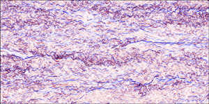
Figure 3. Normalised vertical density gradient  $\partial _{z}\rho ^{\prime }/\vert \partial _{z}\bar {\rho } \vert$ (a,c,e,g) and associated segmented fields (b,d,f,h), for simulations P1F200 (a,b), P1F050 (c,d), P7F200 (e,f) and P7F050 (g,h). The strongly stratified interfaces (SINT) are depicted in blue, the small-scale structures (LAM) in orange, the larger-scale density inversions (INV) in red and the weakly stably stratified regions (WINT) in purple.
3. Density field segmentation methodology
Following Couchman et al. (Reference Couchman, de Bruyn Kops and Caulfield2023), we are interested in the contribution to mixing of the emergent stably stratified interfaces appearing in the density field and how this contribution varies as a function of  $Pr$ and $Fr$. As $Pr$ increases, we expect finer structures to arise in the intervening well-mixed regions and we also are interested in understanding how these structures shape the mixing properties of the flow. Therefore, prior to any analysis, the flow is segmented into four different categories based on the local (vertical) density gradient $\partial _{z}\rho$ as well as the neighbouring (vertical) structure of the flow. We apply the following methodology, as summarised in figure 2:
(i) Stably stratified interfaces. We sort vertical density profiles by values of the density $\rho$ in order to create statically stable density profiles $\rho ^{\ast }(\boldsymbol {x})$. We identify points of the dataset whose values of the density remain unaltered by the sorting procedure, i.e. points that satisfy $\rho (\boldsymbol {x}) = \rho ^{*}(\boldsymbol {x})$. These points are by definition statically stable and have relatively high values of the background buoyancy gradient $N_{\ast }^{2} := - g/(\rho _{0}N_{0}^{2})\partial _{z} \rho ^{\ast }$ (see figure 2b–d) and correspond to stably stratified interfaces lying between relatively well-mixed regions, such as those reported by Couchman et al. (Reference Couchman, de Bruyn Kops and Caulfield2023) for the P1F200 dataset. We thus refer to such points as belonging to the INT (‘interface’) cluster, which is further subdivided into relatively strongly stratified (SINT) and relatively weakly stratified (WINT) interfaces, for $N_{\ast }^{2} > 1$ and $N_{\ast }^{2} \leq 1$ respectively.
(ii) Relatively well-mixed layers. We subdivide points that are altered by the sorting procedure (i.e. are not within an interface INT) into two categories depending on the local density gradient
$\partial _{z} \rho$ and neighbouring structure of the (unsorted) density field $\rho$, in particular relative to $L_T$, the Taylor microscale of the flow. Parameter $L_T$ describes the scale at which viscosity starts to affect the development of turbulent eddies significantly, defined (dimensionally) as $L_T:= \sqrt { 10 \nu {\mathcal {K}} /\epsilon }$, where ${\mathcal {K}}$ is the volume-averaged turbulent kinetic energy. As illustrated in figure 2(c), by considering a point in the dataset at vertical coordinate $z_{c}$ with associated density $\rho _{c} := \rho (z_{c})$ satisfying $\partial _{z} \rho (z_{c})> 0$, we define $z_{+}$ as the closest point moving upwards for which $\rho (z_{+}) = \rho _{c}$. As equality is difficult to ensure numerically, we define
(3.1)Similarly, if\begin{equation} z_{+} := \min\{z > z_{c} \mid \rho(z) \leq \rho(z_{c})\}. \end{equation}$\partial _{z} \rho (z_{c}) < 0$, we define $z_{-} := \min \{z < z_{c} \mid \rho (z) \geq \rho (z_{c})\}$. If $\lvert z_{c} - z_{+} \rvert \leq L_{T}$ (or $\lvert z_{c} - z_{-} \rvert \leq L_{T}$ depending on the local value of the density gradient), we have identified a relatively small-scale structure in the density field, such as a blob or stretched ‘lamella’ as discussed in detail by Villermaux (Reference Villermaux2019), which is strongly affected by viscosity. Therefore we classify these structures as belonging to the LAM (‘lamella’) cluster. Conversely, if $\lvert z_{c} - z_{+} \rvert > L_{T}$ (or $\lvert z_{c} - z_{-} \rvert > L_{T}$), we have identified a point belonging to a relatively large-scale density inversion largely unaffected by viscosity, and so we classify it as being in the INV (‘inversion’) cluster. This algorithm is applied to all vertical levels $z_{c}$ in a given vertical profile of a simulation, and then for all the profiles in the simulation box. Note that the well-mixed regions can be made up of many ‘aggregating’ lamellae, hence the large vertical extent of the LAM cluster (even though this cluster is made up of relatively thin density structures). Similarly, because of the segmentation algorithm used in this work, only the edges of large-scale density inversions are considered in the INV cluster, the bulk of the inversion being made of smaller-scale (aggregating) lamellae. (Indeed, if $z_{c}$ and $z_{\pm }$ are separated by a distance larger than $L_{T}$, only the point $z_{c}$ will be considered in INV but not all the points between $z_{c}$ and $z_{\pm }$, these points being perhaps part of smaller-scale structures.) These edges correspond to the region of maximal (vertical) density gradient in the inversion and hence to the maximal contribution to the statistics of $\chi _{0}$ within the inversion (as is shown in § 4; this fact has also been demonstrated experimentally – see Hult et al. (Reference Hult, Troy and Koseff2011) for instance), motivating further our choice of clusters. Note that the small-scale structure of the relatively well-mixed regions is potentially a consequence of the breakdown of various instabilities, such as the Kelvin–Helmholtz one. Because we are considering only one snapshot in time (at statistical steady state), we cannot further check this hypothesis.


This segmentation methodology, summarised in figure 2, is applied to the four datasets considered in this work, as shown in figure 3.
4. Cluster properties
4.1. Contributions to $\chi$

We consider the relative importance of each cluster defined in § 3 in terms of their contribution to the local and bulk mixing properties of the flow, as described by local  $\chi _0$ and volume-averaged $\chi$. We particularly focus on the role of ‘extreme’ mixing events and therefore sort the data by decreasing values of $\chi _0$, defining a sorted vector $\boldsymbol {\chi }_0^{*} = (\chi _{0}^{0*}, \ldots, \chi _{0}^{M*})$, where $M$ is the number of points in the dataset and $\chi _{0}^{0*}$ and $\chi _{0}^{M*}$ are the greatest and lowest values of $\chi _{0}$ found in the dataset, respectively. This vector can be used to construct the normalised cumulative contribution to $\chi$ as
 \begin{equation} \forall n \in \{1, \ldots, M\}, \quad \chi^{c}(n) := \frac{1}{\chi}\sum_{i=1}^{n}\chi_{0}^{i*}. \end{equation}
The cumulative contribution  $\chi ^{c}$ is plotted in figure 4 for each dataset (solid black line), highlighting the fact that the dominant contribution to $\chi$ is generated by a relatively small set of localised ‘extreme’ events, regardless of $Fr$ and $Pr$. More specifically, for the four sets of parameters considered in this work, approximately $80\,\%$ of the contribution to $\chi$ is contained within the first $10\,\%$ of the points sorted by decreasing values of $\chi _0$ (and hence $10\,\%$ of the box volume). Similar statistics are observed in oceanographic data (Couchman et al. Reference Couchman, Wynne-Cattanach, Alford, Caulfield, Kerswell, MacKinnon and Voet2021).

Figure 4. Normalised cumulative contribution to  $\chi$ (black line; see (4.1)) for each simulation: (a) P1F200, (b) P1F050, (c) P7F200 and (d) P7F050. Data points are assigned to 20 equal-volume bins, sorted by decreasing $\chi _0$ and clustered using the method presented in § 3. For each bin, we compute the relative contribution of each cluster to $\langle \chi \rangle _{{bin}}$, as shown by the heights of the coloured regions. For each bin, we compute the (arithmetic) mean value of $\varGamma _0 := \chi _0 / \epsilon _0$ for each cluster (dashed lines). (e) Total contributions to $\chi$ from each cluster for the four simulations.
The total contribution of each cluster to bulk  $\chi$ is shown in figure 4(e). We also assign the data points sorted by values of $\chi _0$ into $n=20$ equal-volume bins, in order to calculate a relative contribution of points in each cluster to the bin-volume-averaged $\langle \chi \rangle _{{bin}} := \sum _{{bin}}\chi _0/(V/n)$, where $V$ is the total number of points in the domain, as illustrated by coloured shading in figure 4(a–d). Focusing on the $Pr = 1$ case, the contribution (figure 4e) from the strongly stratified interfaces (SINT cluster) to bulk $\chi$ is roughly 25 %–35 %, whereas the contribution from small-scale structures (LAM) reaches ${\sim }60\,\%$. As $Fr$ decreases and stratification strengthens, the total contribution from large-scale inversions (INV) shrinks from ${\sim }10\,\%$ for $Fr=2$ to less than $3\,\%$ for $Fr=0.5$, possibly due to the suppression of large-scale overturnings by relatively strong stratification. We observe similar trends for the relative contributions in each bin. In increasing the Prandtl number from $Pr=1$ to $7$, strong interfaces become (perhaps unsurprisingly) finer (figure 3f,h) and their total contribution shrinks to about $10\,\%$, whereas the total contribution from small-scale structures in ‘lamella’ (LAM) increases to about 80 %–90 %. The total contribution from large-scale inversions does not exceed $10\,\%$. Again, we observe similar trends in the relative contributions as $\chi _0$ decreases.
4.2. Statistics of $\varGamma$

For each bin in figure 4, we compute a mean value of the (local) flux coefficient  $\varGamma _0 := \chi _0 / \epsilon _0$ associated with each cluster (see dashed lines), although such mean values of ratios of local quantities should always be treated with caution. The leftmost bins (corresponding to the most ‘extreme’ values of $\chi _0$) have the largest values of $\varGamma _0$ (of order unity, significantly above the canonical value $\varGamma = 0.2$) suggesting strongly that the extreme mixing events (large $\chi _0$) are not necessarily correlated with extreme dissipation events (large $\epsilon _0$). Among the extreme events in $\chi _0$, those in the strongly stratified interfaces (SINT) cluster correspond to the largest mean values of $\varGamma _0$ (as suggested by Couchman et al. (Reference Couchman, de Bruyn Kops and Caulfield2023) for the $Pr=1$, $Fr=2$ case), independently of variations in $Pr$ and $Fr$. This point is further emphasised in figure 5 where we plot the probability density functions (p.d.f.s) of $\log _{10}(\chi _0)$, $\log _{10}(\epsilon _0)$ and $\log _{10}(\varGamma _0)$ for the different clusters and simulations (computed using normalised histograms with $50$ equispaced bins). We also present the statistical mean of $\chi _0$, $\epsilon _0$ and $\varGamma _0$ (computed using normalised histograms with $50$ bins in log-space). Interestingly, the $\chi _{0}$ distributions are skewed towards high values (note that this skewness seems exacerbated for the INV cluster, for reasons presented in § 3) and the $\varGamma _{0}$ ones encompass almost four orders of magnitude, emphasising again the fact that extreme local values of $\chi _{0}$ are important in setting the overall mixing statistics. Note that these statistics are computed using all the data points in the simulation boxes and hence all the resolved length scales. In more practical settings, where all the length scales down to the Batchelor scales are not necessarily accessible, these p.d.f.s might sharpen around their mean. However, the effective coarse-graining induced by the resolution of the measurements might smooth the fields and hence overlook the (very) thin but yet important strongly stratified interfaces (especially in the high-Prandtl-number case where these interfaces are extremely thin), potentially leading to undersampling of important regions of the density field, and raising the important question of what is the relevant scale at which a turbulent density field should be profiled to get mixing statistics right. This question is not addressed here and is left for future work. For each simulation, the statistical mean of the flux coefficient $\varGamma _0$ is maximised for the strongly stratified interfaces (almost twice as large as the statistical mean for the entire dataset), because of relatively low values of $\epsilon _0$ and large values of $\chi _0$. As the Prandtl number increases, the statistical mean of $\varGamma _0$ decreases (a result also observed by Salehipour et al. (Reference Salehipour, Peltier and Mashayek2015)) for both the weakly and strongly stratified cases, for the following (different) reasons.

Figure 5. The p.d.f.s for  $\log _{10}(\chi _0)$ (a,d), $\log _{10}(\epsilon _0)$ (b,e) and $\log _{10}(\varGamma _0)$ (c,f) for the different clusters defined in § 3 and for the four simulations. The statistical mean of each field (without the logarithm) is represented by a colour-coded circle ( $Pr=1$) or triangle ( $Pr=7$). The green dotted vertical line corresponds to the canonical value $\varGamma =0.2$.
In the weakly stratified simulations with  $Fr=2$ (figure 5a–c), density effectively acts as a passive scalar (as can be seen from the weakly stratified scaling of Riley, Metcalfe & Weissman (Reference Riley, Metcalfe and Weissman1981), for instance) and hence the statistics of $\epsilon _0$ do not depend on $Pr$, as can be seen in figure 5(b). However, as $Pr$ increases, the left-hand tails of the $\chi _0$ distributions become more significant, as might be expected for the mixing of an effectively passive scalar, as $\chi _0$ is multiplied by $(Pr\,Re)^{-1}$ where $Re$ is fixed. We note that a widening of the tails of $\partial _{z}\rho ^{\prime }$ (not shown here; see for instance Riley, Couchman & de Bruyn Kops (Reference Riley, Couchman and de Bruyn Kops2023)) effectively rebuilds the right-hand tail of $\chi _0$, explaining why the p.d.f. of $\chi _0$ is not just shifted toward lower values. A more in-depth discussion of this phenomenon is provided by Bragg & de Bruyn Kops (Reference Bragg and de Bruyn Kops2023). As a result of the statistics of $\epsilon _0$ remaining roughly independent of $Pr$ but those of $\chi _0$ decreasing with increasing $Pr$, the statistics of $\varGamma _0$ decrease as $Pr$ increases for the weakly stratified ( $Fr=2$) case.
Conversely, in the strongly stratified simulations with  $Fr=0.5$, buoyancy acts ‘actively’ on the momentum field, as demonstrated for instance by the strongly stratified scaling analysis of Billant & Chomaz (Reference Billant and Chomaz2001). Moreover, as $Pr$ increases, the volume contribution of the small-scale structures (LAM cluster) increases at the expense of the strongly stratified interfaces (SINT) (see figure 4). The LAM structures, which locally are only weakly affected by stratification because they populate the relatively well-mixed regions of the flow, are viscously affected (as their vertical extent is, by definition, smaller than $L_T$) but still significantly disordered. As a result, their local static instability inevitably encourages increased viscous dissipation, and so their enhanced prevalence actually shifts the statistics of $\epsilon _0$ towards higher values for the $Pr=7$ flows as compared with $Pr=1$ (yellow curves, figure 5f). In this sense, enhanced stratification at higher $Pr$ actually makes the flow ‘more turbulent’, reminiscent of the prediction by Pearson & Linden (Reference Pearson and Linden1983) of relatively long-lived ‘approximately horizontal striations’ in high- $Pr$ decaying stratified turbulence. Also, though this is a second-order effect, for the strongly stratified simulations the left-hand tail of the $\chi _0$ distribution once again becomes somewhat more significant as $Pr$ increases. We note that while the forcing scheme endeavours to maintain a constant $Re_b$, bulk $\epsilon$ is slightly mismatched between the two $Pr$ simulations at $Fr=0.5$ (see table 1). Therefore, while increased $Pr$ dramatically changes the relative prevalence of LAM versus SINT structures, part of the observed increase in local $\epsilon _0$ statistics at $Pr=7, Fr=0.5$ is due to the slight mismatch in targeted bulk $\epsilon$ rather than being a purely $Pr$ effect. Importantly, it is apparent in figure 5(e) that the total amount of irreversible mixing for the flow with $Pr=7$ actually slightly increases compared to $Pr=1$ in the more strongly stratified $Fr=0.5$ simulations, essentially because the $Pr=7$ flow is more vigorous, despite the fact that $\varGamma _0$ appears to decrease with increasing $Pr$. Therefore, consideration of $\varGamma _0$, or even $\varGamma :=\chi /\epsilon$ (constructed from volume-averaged dissipation rates), in isolation should be treated with caution.
5. Discussion
We have analysed the influence of the Prandtl number  $Pr$ and Froude number $Fr$ on density structures in forced turbulent stratified flows and their contribution to irreversible scalar mixing properties. Using fully resolved DNS data and a flow segmentation algorithm based on the local value of the (vertical) density gradient and the local (vertical) structure of the density field, we have extracted distinct regions of the turbulent density field – interfaces (both relatively strong and relatively weak) separating well-mixed density layers made up of both small-scale lamellar structures and larger scale density inversions – and analysed their contribution to the bulk value of the destruction rate of buoyancy variance $\chi$ and to the statistics of the (locally evaluated) flux coefficient $\varGamma _0$.
As  $Pr$ increases, the strongly stratified density interfaces become finer and their contribution to average values of $\chi$ decreases at the expense of the small-scale lamellar structures in the relatively well-mixed density layers. However, similarly to the flow with $Pr=1$ (Couchman et al. Reference Couchman, de Bruyn Kops and Caulfield2023), these structures are ‘quiescent’, yet mixing hotspots. The points in these structures associated with the largest values of (local) $\chi _0$ are associated with extreme values of $\varGamma _0$ and hence with relatively low values of $\epsilon _0$. More generally, the flux coefficient associated with strongly stratified structures is (in an averaged sense) essentially twice as large as its value for the three other segmented regions, regardless of the values of $Pr$ and $Fr$. All in all, strongly stratified interfaces are therefore characterised by relatively large values of $\chi _0$ and relatively weak values of $\epsilon _0$ compared with the other density structures considered in this work and are therefore likely to be overlooked if considering $\epsilon _0$ (or indeed the volume average $\epsilon$) alone as a proxy for significant irreversible mixing.
As is becoming increasingly well appreciated, a universal value of  $\varGamma$ is not able to capture the complex and inhomogeneous structures of the density and density gradient turbulent fields. Moreover, our description of the density fields as well as consideration of the considered mixing regime (i.e. ‘passive’ mixing at higher $Fr$ as compared with ‘active’ mixing at lower $Fr$) offers a potential explanation for the empirical observation that the ‘mixing efficiency’ $\varGamma /(1+\varGamma )$ decreases with $Pr$. On the one hand, mixing in the relatively weakly stratified case can be described as ‘passive’: the velocity field and hence $\epsilon _0$ are largely unaffected by $Pr$ but the small-scale structure of the density field evolves as $Pr$ increases from $1$ to $7$ in a way that results in a decrease in $\chi _0$ and thus the flux coefficient $\varGamma _0$. On the other hand, mixing in the relatively strongly stratified case can be thought of as ‘active’, with the density field and its small-scale lamellar structure having a leading-order impact on the rate at which the turbulent kinetic energy is dissipated ( $\epsilon _0$), ultimately leading to a decrease in $\varGamma _0$ as $Pr$ increases. This shows another way in which a focus on the flux coefficient can be misleading. Since the decrease in $\varGamma _0$ is actually principally related to an increase in $\epsilon _0$, the total amount of mixing (quantified by $\chi$) actually increases in the higher- $Pr$, strongly stratified flow considered here. Accurately predicting the flux coefficient being crucial to modelling mixing in large-scale ocean models for instance (through turbulent diffusivities for instance), our study emphasises the need to better understand the dependence of this parameter on the small-scale structure of the density field. Another key result of our analysis is that the Prandtl number $Pr$ has a leading-order impact (at least compared with the Froude number $Fr$) on the density field structures and their mixing properties, further emphasising the need to take this parameter into account when ‘measuring mixing’, a process that is inherently a diffusive one (Villermaux Reference Villermaux2019; Caulfield Reference Caulfield2021) and that affects the density field.
We here considered steady-state forced stratified turbulent flows, and so it would now be interesting to apply our segmentation and associated mixing contribution analysis to time-dependent decaying stratified turbulent flows. For example, what is the fate of the different emerging structures? Can a separate analysis of the temporal evolution of each structure help us better understand the mixing history of a stratified turbulent flow as a whole and unveil the fundamental rules of stratified mixing? These are questions left for future work.
Funding
This project received funding from the European Union's Horizon 2020 research and innovation programme under Marie Sklodowska-Curie grant agreement no. 956457 and used resources of the Oak Ridge Leadership Computing Facility at the Oak Ridge National Laboratory, supported by the Office of Science of the US Department of Energy under contract no. DE-AC05-00OR22725. S.d.B.K. was supported under US Office of Naval Research grant number N00014-19-1-2152.
Declaration of interests
The authors report no conflict of interest.


 Open access