


1. Introduction
Surprisingly, no general method exists to establish whether or not an exact inviscid steady state solution approximates the behaviour of a real viscous fluid at high Reynolds number. This may be due to the widely held view that viscous effects are either a regular perturbation or a singular perturbation in the form of an interior or boundary layer. In fact, viscous effects always represent a singular perturbation for rotational flows even in the absence of interior/boundary layers. In the high-Reynolds-number limit, small viscous terms in the Navier–Stokes equations accumulate over time to have a leading-order effect. Therefore, the amplitude of the rotational flow must satisfy secularity conditions determined by viscosity. The absence of research on this topic is in stark contrast to other fields, such as wall-bounded shear flows at high Reynolds number. Boundary-layer theory has achieved significant success in wall-bounded shear flows, for example, uniform flow over a semi-infinite plate (Smith & Burggraf Reference Smith and Burggraf1985; Smith, Doorly & Rothmayer Reference Smith, Doorly and Rothmayer1990), Hagen–Poiseuille flow (Smith & Bodonyi Reference Smith and Bodonyi1982) or vortex–wave interaction theory (Hall & Smith Reference Hall and Smith1991).
In this paper, we will investigate whether or not a steady rotational solution of the Euler equations can approximate a real flow at large Reynolds number. The techniques described in this article are irrelevant for irrotational flows, because irrotational flows are exact solutions of the full Navier–Stokes equations. Exact inviscid steady state solutions can provide valuable physical insight and serve to validate the accuracy of numerical solutions, but they are of greatest interest when they approximate the behaviour of a real fluid in the high-Reynolds-number limit. Physical inviscid steady state solutions may approximate either steady states or quasi-steady states of the Navier–Stokes equations, a quasi-steady state being defined to be a leading-order solution which only varies on a long time scale. We will investigate both situations due to the following considerations. Stable steady states are of the greatest interest, but unstable steady states also play an important role as intermediate states in flow evolution. Long-lived quasi-steady states have been shown to be the destination of two-dimensional turbulence in a periodic domain (Matthaeus et al. Reference Matthaeus, Stribling, Martinez, Oughton and Montgomery1991a,Reference Matthaeus, Stribling, Martinez, Oughton and Montgomeryb; Montgomery et al. Reference Montgomery, Matthaeus, Stribling, Martinez and Oughton1992), so these solutions are also of physical significance. In order to be a quasi-steady state, an exact inviscid steady state solution must have at least one free parameter.
Vortices are present everywhere in nature and technology. As examples, vortical structures are relevant to the understanding of atmospheric and oceanic circulations, mesoscale vortices being found everywhere in the atmosphere and the oceans which cover the Earth. The most common vortices in geophysical fluid dynamics are monopoles and dipoles. Therefore, it is important to study isolated vortices (Wu, Ma & Zhou Reference Wu, Ma and Zhou2006).
Many exact inviscid steady states have been found by many methods (Saffman Reference Saffman1992; Meleshko & van Heijst Reference Meleshko and van Heijst1994; Wu et al. Reference Wu, Ma and Zhou2006). However, certain fundamental solutions of the Euler equations, such as the point vortex and the straight line vortex, are not susceptible to our analysis. In this article, we consider four exact inviscid steady states with the first two being considered together due to their similarity.
• Stuart (Reference Stuart1967) determined an exact inviscid solution in the form of a steady single vortex row with finite cores. Each core resides in a two-dimensional rectangular domain which is periodic in the streamwise direction and infinite in the lateral direction. Mallier & Maslowe (Reference Mallier and Maslowe1993) presented the corresponding result for a steady row of counter-rotating vortices. Both of these exact solutions have a single free parameter, so they could represent quasi-steady states of the Navier–Stokes equations.
• Hill (Reference Hill1894) discovered an exact inviscid solution in the form of an axisymmetric steady vortex ring enclosed within a sphere. With the addition of a pressure correction, the exact inviscid solution may be converted to an exact solution of the Navier–Stokes equations (Saffman Reference Saffman1992). The addition of an appropriate correction is one of the few existing methods to establish that an exact inviscid steady state solution approximates the behaviour of a real viscous fluid. Unfortunately, in almost all other cases, it is impossible to determine whether or not a first correction exists. Hill's spherical vortex will be used to check our more general approach. Moffatt (Reference Moffatt1969) extended Hill's spherical vortex to allow for non-zero azimuthal velocity, but this solution of the Euler equations will not be considered in this article. Moffatt & Moore (Reference Moffatt and Moore1978) and Protas & Elcrat (Reference Protas and Elcrat2016) investigated the stability of Hill's spherical vortex to axisymmetric disturbances. Crowe, Kemp & Johnson (Reference Crowe, Kemp and Johnson2021) recently predicted the decay of the vortex speed and radius of Hill's spherical vortex in a weakly rotating flow due to the radiation of inertial waves.
• Lamb (Reference Lamb1895) and Chaplygin (Reference Chaplygin1903) independently found an exact inviscid solution in the form of a vortex dipole enclosed within a circle. The vortex profiles have been shown to be in good agreement with numerical solutions of the two-dimensional Navier–Stokes equations (Couder & Basdevant Reference Couder and Basdevant1986). This exact solution has a free parameter, so it could also represent a quasi-steady state of the Navier–Stokes equations.
These and other classical Euler solutions have been widely used to analyse the stability of vortex flows and wakes (Pierrehumbert & Widnall Reference Pierrehumbert and Widnall1982; Dauxois, Fauve & Tuckerman Reference Dauxois, Fauve and Tuckerman1996; Julien, Chomaz & Lasheras Reference Julien, Chomaz and Lasheras2002), the interaction of a vortex and a bubble (Higuera Reference Higuera2004) or a shock wave (Pirozzoli Reference Pirozzoli2004). They are also associated with the study of coherent structures in turbulence, which has fostered the hope that the study of vortices will also lead to a better understanding of turbulent flows (Saffman Reference Saffman1992). As such, it is important to know if they describe real viscous fluid flows.
For many years, expansions in terms of the amplitude have been used to investigate oscillations in fluid mechanics. For example, Stuart (Reference Stuart1960) produced seminal work on the weakly nonlinear analysis of waves in plane Poiseuille flow. More recently, quasi-steady states of finite amplitude have been studied in fluid mechanics using the asymptotic techniques employed in this article. Kuzmak (Reference Kuzmak1959) introduced the strongly nonlinear analysis of ordinary differential equations. His technique has recently been applied to the Rayleigh–Plesset equation in order to model the viscous decay of oscillating spherical bubbles (Smith & Wang Reference Smith and Wang2017) and to the Keller–Miksis equation in order to describe the radiative decay of oscillating spherical bubbles (Smith & Wang Reference Smith and Wang2018). Kuzmak's method has also been applied to the three-dimensional Navier–Stokes equations to successfully predict the viscous decay of an oscillating drop (Smith Reference Smith2010). Kuzmak's method has not been previously applied to steady states in fluid mechanics or in any other field.
Our study is based on the asymptotic analysis of the Navier–Stokes equation in terms of the reciprocal of the Reynolds number. The leading-order solutions are the steady Euler equations. By exploring the existence of the solutions to the first-correction equations, we establish the form of the solvability conditions (modulation equations) which control the amplitude of steady states (quasi-steady states) at high Reynolds number. For travelling waves in two-dimensional plane Poiseuille flow and two-dimensional Kolmogorov flow, the modulation equations have been shown to be single equations for averaged momentum and energy and a family of equations for averaged powers of vorticity (Smith & Wissink Reference Smith and Wissink2015, Reference Smith and Wissink2018). Modulation equations are a property of the equations and not of the solutions being considered, so these modulation equations apply whenever the leading-order problem is a two-dimensional travelling wave. These equations will also control the amplitude of two-dimensional steady states and quasi-steady states. The question is whether or not there exist additional solvability conditions (modulation equations) when we consider steady states (quasi-steady states).
The contents of the paper will now be outlined. Stuart cats’ eyes and Mallier–Maslowe vortices are studied in § 2, Hill's spherical vortex in § 3 and the Lamb–Chaplygin dipole in § 4. In each of these three sections, asymptotic analysis based on the Fredholm alternative is applied to determine whether or not viscous corrections exist. Finally, § 5 gives a brief discussion of the results.
2. Stuart cats’ eyes and Mallier–Maslowe vortices
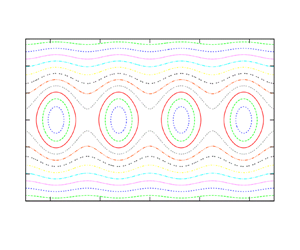
Stuart cats’ eyes (Stuart Reference Stuart1967) and Mallier–Maslowe vortices (Mallier & Maslowe Reference Mallier and Maslowe1993) are two exact solutions to the Euler equations describing a row of vortices. Their streamlines are displayed in figure 1, with Stuart cats’ eyes being a row of co-rotating vortices and Mallier–Maslowe vortices being a row of counter-rotating vortices. The two classical solutions have been widely used to analyse the stability of the von Kármán vortex street, a repeating pattern of swirling vortices which appear in the wake of an object placed in a flowing stream of fluid (Pierrehumbert & Widnall Reference Pierrehumbert and Widnall1982; Dauxois et al. Reference Dauxois, Fauve and Tuckerman1996; Julien et al. Reference Julien, Chomaz and Lasheras2002). We will discuss if these two classic solutions approximate solutions to the Navier–Stokes equation.

2.1. Introduction
In this subsection, we will describe the mathematical model for Stuart cats’ eyes and Mallier–Maslowe vortices. We consider the two-dimensional Navier–Stokes equations and the continuity equation for incompressible Newtonian fluids in the form
 $$\begin{gather} \frac{\partial u}{\partial t} + u \frac{\partial u}{\partial x} + v \frac{\partial u}{\partial y} + \frac{\partial p}{\partial x}={-} \epsilon \frac{\partial \omega}{\partial y}, \end{gather}$$
 $$\begin{gather}\frac{\partial v}{\partial t} + u \frac{\partial v}{\partial x} + v \frac{\partial v}{\partial y} + \frac{\partial p}{\partial y}=\epsilon \frac{\partial \omega}{\partial x}, \end{gather}$$
 $$\begin{gather}\frac{\partial u}{\partial x}+\frac{\partial v}{\partial y}=0, \end{gather}$$
in which  $(x,y)^\textrm {T}$ are Cartesian coordinates, $t$ is time, $(u,v)^\textrm {T}$ is the velocity vector, $p$ is the pressure, $\omega$ is the vorticity given by
 \begin{equation} \omega = \frac{\partial v}{\partial x} - \frac{\partial u}{\partial y}, \end{equation} $\epsilon =1/Re$ is the reciprocal of the Reynolds number $Re$ and $0 < \epsilon \ll 1$ for high-Reynolds-number flows. The periodic boundary conditions in the streamwise direction are
 \begin{equation} [u,v,p](0, y, t) = [u,v,p](2 {\rm \pi}, y, t). \end{equation}
The far-field boundary conditions in the lateral direction for Stuart cats’ eyes are
 \begin{equation} u \rightarrow \pm 1\quad \text{as } y \rightarrow \pm \infty, \quad v \rightarrow 0 \quad\text{as } y \rightarrow \pm \infty, \end{equation}
and for Mallier–Maslowe vortices are
 \begin{equation} u \rightarrow 0 \quad \text{as } y \rightarrow \pm \infty, \quad v \rightarrow 0 \quad \text{as } y \rightarrow \pm \infty. \end{equation}
2.2. The leading-order solution
We will first perform the perturbation procedure on the nonlinear system (2.1)–(2.3) with (2.4a,b) or (2.5a,b). The solutions for Stuart cats’ eyes and Mallier–Maslowe vortices will then be obtained in §§ 2.2.1 and 2.2.2, respectively. We introduce expansions of the form
 \begin{equation} u \sim u_0 + \epsilon u_1,\quad v \sim v_0 + \epsilon v_1,\quad p \sim p_0 + \epsilon p_1 ,\quad \omega \sim \omega_0 + \epsilon \omega_1 , \end{equation}
as  $\epsilon \rightarrow 0$. At leading order, for the quasi-steady state, we obtain
 \begin{equation} \bar{L} u_0 + \frac{\partial p_0}{\partial x} = 0,\quad \bar{L} v_0 +\frac{\partial p_0}{\partial y} = 0, \quad \frac{\partial u_0}{\partial x} + \frac{\partial v_0}{\partial y} = 0, \end{equation}
with the differential operator
 \begin{equation} \bar{L}= u_0 \frac{\partial}{\partial x} +v_0 \frac{\partial}{\partial y}. \end{equation}
We take the  $x$-derivative of the second equation in (2.7a–c) minus the $y$-derivative of the first equation in (2.7a–c) to find that $\bar {L} \omega _0 = 0$. A streamfunction $\psi$ is defined by the equations
 \begin{equation} u_0 = \frac{\partial \psi}{\partial y}, \quad v_0 ={-} \frac{\partial \psi}{\partial x}, \end{equation}
so that the third equation in (2.7a–c) is automatically satisfied and the vorticity equation may be rewritten as
 \begin{equation} \frac{\partial \psi}{\partial y} \frac{\partial \omega_0}{\partial x} -\frac{\partial \psi}{\partial x} \frac{\partial \omega_0}{\partial y}=0. \end{equation}
2.2.1. Stuart cats’ eyes
The Stuart cats’ eyes correspond to the solution of (2.10) given by  $\omega _0 = - \exp \{- 2 \psi \}$, so that $\psi$ satisfies the partial differential equation
 \begin{equation} \frac{\partial^2 \psi}{\partial x^2} + \frac{\partial^2 \psi}{\partial y^2} = \exp \{- 2 \psi \} \end{equation}
with the boundary conditions
 \begin{equation} \psi(0, y, \tilde{t})=\psi(2 {\rm \pi}, y, \tilde{t}), \quad \psi \rightarrow \pm y \text{ as } y \rightarrow \pm \infty. \end{equation}
The Stuart cats’ eyes are a solution of this boundary value problem in the form
 \begin{equation} \psi(x, y, \tilde{t}) = \log [ C(\tilde{t}) \cosh(y) + A(\tilde{t}) \cos(x) ], \end{equation}
where  $C(\tilde {t})>1$, $A(\tilde {t})=(C(\tilde {t})^2-1)^{1/2}>0$ and $\tilde {t} = \epsilon t$. The streamlines for $C(\tilde {t})=1.1$ are shown in figure 1(a). We deduce that
 \begin{equation} u_0 = \frac{C(\tilde{t}) \sinh(y)}{C(\tilde{t}) \cosh(y) + A(\tilde{t}) \cos(x)}, \quad v_0 = \frac{A(\tilde{t}) \sin(x)}{C(\tilde{t}) \cosh(y) + A(\tilde{t}) \cos(x)}. \end{equation}
The leading-order kinetic energy is given by  $E_0 = (u_0^2+v_0^2)/2$. We note that $\psi$, $v_0$ and $\omega _0$ ( $u_0$) are even (odd) in $y$ about $y=0$. At leading order, the Bernoulli function, $H$, may be written in the form
 \begin{equation} H(\psi) = p_0 + E_0 = \tfrac{1}{2} \{ 1 - \textrm{e}^{{-}2 \psi} \}. \end{equation}
2.2.2. Mallier–Maslowe vortices
The Mallier–Maslowe vortices correspond to the solution of (2.10) given by  $\omega _0 = (1-B^2)\sinh \{ 2 \psi \}/2$, so that $\psi$ satisfies the partial differential equation
 \begin{equation} \frac{\partial^2 \psi}{\partial x^2} + \frac{\partial^2 \psi}{\partial y^2} ={-}\frac{(1-B^2)}{2} \sinh \{ 2 \psi \} \end{equation}
with the boundary conditions
 \begin{equation} \psi(0, y, \tilde{t})=\psi(2 {\rm \pi}, y, \tilde{t}), \quad \psi \rightarrow 0 \text{ as } y \rightarrow \pm \infty, \end{equation}
where  $0< B(\tilde {t})<1$ and $\tilde {t} = \epsilon t$. The Mallier–Maslowe vortices are a solution of this boundary value problem in the form
 \begin{equation} \psi(x, y, \tilde{t}) = \log \left [ \frac{\cosh(B(\tilde{t}) y) - B(\tilde{t}) \cos(x)}{\cosh(B(\tilde{t}) y) + B(\tilde{t}) \cos(x)} \right ] ={-}2 \text{arctanh} \left [ \frac{B(\tilde{t}) \cos(x)}{\cosh(B(\tilde{t}) y)} \right ]. \end{equation}
The streamlines for  $B(\tilde {t})=1/2$ are shown in figure 1(b). We deduce that
 \begin{equation} u_0 = \frac{2 B(\tilde{t})^2 \cos(x) \sinh(B(\tilde{t}) y)}{\cosh^2(B(\tilde{t}) y) - B(\tilde{t})^2 \cos^2(x)}, \quad v_0 ={-}\frac{2 B(\tilde{t}) \sin(x) \cosh(B(\tilde{t}) y)}{\cosh^2(B(\tilde{t}) y) - B(\tilde{t})^2 \cos^2(x)}. \end{equation}
We note that  $\psi$, $v_0$ and $\omega _0$ ( $u_0$) are even (odd) in $y$ about $y=0$. Furthermore, these solutions are such that $\psi$, $u_0$ and $\omega _0$ ( $v_0$) are odd (even) in $x$ about zeros of $u_0$. At leading order, the Bernoulli function, $H$, may be written in the form
 \begin{equation} H(\psi; B) = p_0 + E_0 ={-}\frac{(1-B^2)}{4} \cosh \{ 2 \psi \}. \end{equation}
2.3. The first correction
We now derive the linear problem for the first correction and the conditions (2.30) under which it may have a solution. At the next order, we have
 \begin{equation} L \boldsymbol{z} =
\left(\begin{array}{@{}c@{}} \displaystyle -\dfrac{\partial
u_0}{\partial \tilde{t}}-\dfrac{\partial \omega_0}{\partial
y}\\ [10pt] \displaystyle -\dfrac{\partial v_0}{\partial
\tilde{t}}+\dfrac{\partial \omega_0}{\partial x}\\ 0
\end{array}\right), \end{equation}
\begin{equation} L \boldsymbol{z} =
\left(\begin{array}{@{}c@{}} \displaystyle -\dfrac{\partial
u_0}{\partial \tilde{t}}-\dfrac{\partial \omega_0}{\partial
y}\\ [10pt] \displaystyle -\dfrac{\partial v_0}{\partial
\tilde{t}}+\dfrac{\partial \omega_0}{\partial x}\\ 0
\end{array}\right), \end{equation}
in which
 \begin{equation}
L=\left(\begin{array}{@{}ccc@{}} \displaystyle \bar{L} +
\dfrac{\partial u_0}{\partial x} & \displaystyle
\dfrac{\partial u_0}{\partial y} & \displaystyle
\dfrac{\partial}{\partial x}\\[10pt] \displaystyle
\dfrac{\partial v_0}{\partial x} & \displaystyle \bar{L} +
\dfrac{\partial v_0}{\partial y} & \displaystyle
\dfrac{\partial}{\partial y}\\[10pt] \displaystyle
\dfrac{\partial}{\partial x} & \displaystyle
\dfrac{\partial}{\partial y} & \displaystyle 0
\end{array}\right),\quad
\boldsymbol{z}=\left(\begin{array}{@{}c@{}} u_1\\ v_1\\ p_1
\end{array}\right), \end{equation}
\begin{equation}
L=\left(\begin{array}{@{}ccc@{}} \displaystyle \bar{L} +
\dfrac{\partial u_0}{\partial x} & \displaystyle
\dfrac{\partial u_0}{\partial y} & \displaystyle
\dfrac{\partial}{\partial x}\\[10pt] \displaystyle
\dfrac{\partial v_0}{\partial x} & \displaystyle \bar{L} +
\dfrac{\partial v_0}{\partial y} & \displaystyle
\dfrac{\partial}{\partial y}\\[10pt] \displaystyle
\dfrac{\partial}{\partial x} & \displaystyle
\dfrac{\partial}{\partial y} & \displaystyle 0
\end{array}\right),\quad
\boldsymbol{z}=\left(\begin{array}{@{}c@{}} u_1\\ v_1\\ p_1
\end{array}\right), \end{equation}
with the periodic and far-field boundary conditions
 $$\begin{gather} [u_1,v_1,p_1](0, y, \tilde{t}) = [u_1,v_1,p_1](2 {\rm \pi}, y, \tilde{t}), \end{gather}$$
 $$\begin{gather}u_1 \rightarrow 0 \quad \text{as } y \rightarrow \pm \infty, \quad v_1 \rightarrow 0 \quad\text{as } y \rightarrow \pm \infty. \end{gather}$$
A general solution to the linear problem for the first correction (2.21)–(2.23) is very difficult to find. Therefore, we investigate the adjoint problem in order to determine the conditions under which the problem for the first correction has a solution. Following the analysis in Smith (Reference Smith2007), we have an equation with the right-hand side in divergence form
 \begin{align} \boldsymbol{r}^T L \boldsymbol{z} - \boldsymbol{z}^T L^* \boldsymbol{r}&= \frac{\partial}{\partial x} [ u_0 \{ a u_1 + b v_1 \} +a p_1 + c u_1 ] \nonumber\\ &\quad + \frac{\partial}{\partial y} [ v_0 \{ a u_1 + b v_1 \}+ b p_1 + c v_1 ], \end{align}
in which the adjoint operator  $L^*$ and vector $\boldsymbol {r}$ are given by
 \begin{equation}
L^{*}=\left(\begin{array}{@{}ccc@{}} \displaystyle -\bar{L} +
\dfrac{\partial u_0}{\partial x} & \displaystyle
\dfrac{\partial v_0}{\partial x} & \displaystyle -
\dfrac{\partial}{\partial x}\\[10pt] \displaystyle
\dfrac{\partial u_0}{\partial y} & \displaystyle -\bar{L} +
\dfrac{\partial v_0}{\partial y} & \displaystyle
-\dfrac{\partial}{\partial y}\\ [10pt] \displaystyle
-\dfrac{\partial}{\partial x} & \displaystyle
-\dfrac{\partial}{\partial y} & \displaystyle 0
\end{array}\right),\quad
\boldsymbol{r}=\left(\begin{array}{@{}c@{}} a\\ b\\ c
\end{array}\right). \end{equation}
\begin{equation}
L^{*}=\left(\begin{array}{@{}ccc@{}} \displaystyle -\bar{L} +
\dfrac{\partial u_0}{\partial x} & \displaystyle
\dfrac{\partial v_0}{\partial x} & \displaystyle -
\dfrac{\partial}{\partial x}\\[10pt] \displaystyle
\dfrac{\partial u_0}{\partial y} & \displaystyle -\bar{L} +
\dfrac{\partial v_0}{\partial y} & \displaystyle
-\dfrac{\partial}{\partial y}\\ [10pt] \displaystyle
-\dfrac{\partial}{\partial x} & \displaystyle
-\dfrac{\partial}{\partial y} & \displaystyle 0
\end{array}\right),\quad
\boldsymbol{r}=\left(\begin{array}{@{}c@{}} a\\ b\\ c
\end{array}\right). \end{equation}
Equation (2.24) may be integrated to yield
 \begin{equation} \langle \boldsymbol{r}^T L \boldsymbol{z} - \boldsymbol{z}^T L^* \boldsymbol{r} \rangle = 0, \end{equation}
where
 \begin{equation} \langle \ {\bullet}\ \rangle = \int^{2 {\rm \pi}}_{x=0} \int^{\infty}_{y={-}\infty} \ {\bullet}\ \textrm{d} y \,\textrm{d}\kern0.7pt x, \end{equation}
provided that the following conditions are satisfied
 $$\begin{gather} [a,b,c](0, y, \tilde{t})= [a,b,c](2 {\rm \pi}, y, \tilde{t}), \end{gather}$$
 $$\begin{gather}b \rightarrow 0 \quad \text{as } y \rightarrow \pm \infty. \end{gather}$$
It follows from (2.26) that if
 \begin{equation} L^* \boldsymbol{r} = \boldsymbol{0}, \end{equation}
subject to the conditions (2.28), then our linear problem for the first correction (2.21)–(2.23) can only have a solution if
 \begin{equation} \left \langle -a \left [ \frac{\partial \omega_0}{\partial y} + \frac{\partial u_0}{\partial \tilde{t}} \right ] + b \left [ \frac{\partial \omega_0}{\partial x} - \frac{\partial v_0}{\partial \tilde{t}} \right ] \right \rangle=0, \end{equation}
for any  $\boldsymbol {r}=(a,b,c)^\textrm {T}$ in the null space of the adjoint problem. It remains to find the linearly independent solution vectors $\boldsymbol {r}$ and substitute them into (2.30).
Two linearly independent solutions of the adjoint problem (2.29) and (2.28) are
 \begin{equation} \boldsymbol{r}_1 = (0,0,1)^\textrm{T}, \quad \boldsymbol{r}_2 = (1,0,u_0)^\textrm{T}. \end{equation}
One infinite family of linearly independent solutions is given by
 \begin{equation} \boldsymbol{r}_3 = \left(\frac{\partial }{\partial y} (\omega_0^{n-1}), -\frac{\partial }{\partial x} (\omega_0^{n-1}),-\frac{(n-1)}{n} \omega_0^n \right)^\textrm{T}, \end{equation}
for  $n>1$ and $n \in \textrm {I R}$. The vorticity is finite for these flows. The function $\omega _0^n$ is thus continuous on $[-\omega _{max}, \omega _{max}]$, where $\omega _{max}$ bounds the values of vorticity. Given this condition, the Weierstrass approximation theorem ensures that a polynomial
 \begin{equation} p(\omega_0) = a_0 + a_1 \omega_0 + \cdots + a_q \omega_0^q, \end{equation}
exists with  $a_i$ real constants and $q$ a non-negative integer, which uniformly approximates $\omega _0^n$ on $[-\omega _{max}, \omega _{max}]$; that is,
 \begin{equation} p(\omega_0) - \hat{\epsilon} < \omega_0^n < p(\omega_0) + \hat{\epsilon}, \end{equation}
for any  $\hat {\epsilon }>0$. We note that $a_0=0$ in this case and consider the vector space of polynomials $p(\omega _0)$ over the field of real numbers. If we construct a basis for this space of polynomials $\{ \omega _0^n \mid n \in \textrm {I N} \}$, then all functions in $\{ \omega _0^m \mid m \in \textrm {I R}, \ m > 1 \}$ are uniformly approximated by our basis. Hence, it is sufficient to construct modulation equations for the basis, taking the powers to be natural numbers. A countably infinite family of linearly independent solutions of the adjoint problem (2.29) and (2.28) have been deduced; that is, $\boldsymbol {r}_3$ for $n$ in the natural numbers.
A further infinite family of linearly independent solutions is given by
 \begin{equation} \boldsymbol{r}_4 = \left(f(\psi) u_0, f(\psi) v_0, \int^{\psi} f(s) H^{\prime} (s) \, \textrm{d} s \right)^\textrm{T}, \end{equation}
where  $f(s)$ is a differentiable function. As $f(s)$ is not defined on a bounded interval, the Weierstrass approximation theorem does not apply in this case.
2.4. Modulation equations
The first solution to the adjoint problem,  $\boldsymbol {r}_1$, corresponds to a trivial modulation equation. The second solution results in a degenerate modulation equation due to the parity in $y$ of both the Stuart cats’ eyes and Mallier–Maslowe vortices. Only the third and fourth solutions correspond to physical modulation equations to be described in the following.
2.4.1. Vorticity to the power  $n$ modulation equations

If we substitute the third vector  $\boldsymbol {r}_3$ into (2.30), then we obtain our first secularity conditions
 \begin{equation} \left \langle -\frac{\partial}{\partial y}(\omega_0^{n-1}) \left [ \frac{\partial \omega_0}{\partial y} + \frac{\partial u_0}{\partial \tilde{t}} \right ] -\frac{\partial}{\partial x}(\omega_0^{n-1}) \left [ \frac{\partial \omega_0}{\partial x} - \frac{\partial v_0}{\partial \tilde{t}} \right ] \right \rangle=0. \end{equation}
After integration by parts in both  $x$ and $y$, we derive
 \begin{equation} \left \langle \omega_0^{n-1} \frac{\partial}{\partial y} \left [ \frac{\partial \omega_0}{\partial y} + \frac{\partial u_0}{\partial \tilde{t}} \right ] + \omega_0^{n-1} \frac{\partial}{\partial x} \left [ \frac{\partial \omega_0}{\partial x} - \frac{\partial v_0}{\partial \tilde{t}} \right ] \right \rangle=0. \end{equation}
This may be rewritten as the modulation equations
 \begin{equation} \frac{\textrm{d} }{\textrm{d} \tilde{t}} \left \langle \omega_0^n \right\rangle = \left \langle n \omega_0^{n-1} \left [ \frac{\partial^2 \omega_0}{\partial x^2} + \frac{\partial^2 \omega_0}{\partial y^2} \right ] \right\rangle, \end{equation}
for  $n \in \textrm {I N}$.
2.4.2. Generalized energy modulation equations
If we substitute the fourth vector  $\boldsymbol {r}_4$ into (2.30), then we obtain the further secularity conditions
 \begin{equation} \left \langle f(\psi) u_0 \left [ -\frac{\partial \omega_0}{\partial y} - \frac{\partial u_0}{\partial \tilde{t}} \right ] + f (\psi) v_0 \left [ \frac{\partial \omega_0}{\partial x} - \frac{\partial v_0}{\partial \tilde{t}} \right ] \right \rangle=0. \end{equation}
This may be rewritten as
 \begin{equation} \left \langle f (\psi) \left [ \frac{\partial E_0}{\partial \tilde{t}} + u_0 \frac{\partial \omega_0}{\partial y} - v_0 \frac{\partial \omega_0}{\partial x} \right ] \right \rangle=0. \end{equation}
Equations (2.38) and (2.40) are termed as the vorticity to the power  $n$ modulation equations and the generalized energy modulation equations, respectively. They are necessary conditions for the solutions of the Euler equations to approximate the solutions for the Navier–Stokes equation.
2.5. Inconsistency of the steady state
We consider the energy solvability condition for the steady state by taking  $\partial E_0 / \partial \tilde {t} = 0$ and $f (\psi )=1$ in (2.40); that is,
 \begin{equation} \left \langle v_0 \frac{\partial \omega_0}{\partial x}- u_0 \frac{\partial \omega_0}{\partial y} \right \rangle=0. \end{equation}
We will show that both Stuart cats’ eyes and Mallier–Maslowe vortices do not satisfy this steady solvability condition (2.41) in §§ 2.5.1 and 2.5.2, respectively. Thus, they do not approximate a steady state of the Navier–Stokes equations.
2.5.1. Stuart cats’ eyes
If we substitute for the leading-order solution (2.13)–(2.15), the solvability condition (2.41) becomes
 \begin{equation} \int^{2 {\rm \pi}}_{x=0} \int^{\infty}_{y={-}\infty} - \frac{2 \{ A^2 \sin^2 (x) + C^2 \sinh^2(y) \}}{[C \cosh(y) + A \cos(x)]^4} \, \textrm{d} y \,\textrm{d}\kern0.7pt x=0. \end{equation}
The left-hand side of this solvability condition is non-zero and the solvability condition is not satisfied. The problem for the first correction (2.21)–(2.23) does not have a solution by the Fredholm alternative. Stuart cats’ eyes are solutions to the steady Euler equations, but are not a leading-order solution to the steady Navier–Stokes equations for high-Reynolds-number flows. As such, Stuart cats’ eyes do not approximate a steady state of the Navier–Stokes equations.
2.5.2. Mallier–Maslowe vortices
If we substitute for the leading-order solution (2.18)–(2.20), the solvability condition (2.41) becomes
 \begin{equation} \int^{2 {\rm \pi}}_{x=0} \int^{\infty}_{y={-}\infty} - (1-B^2) E_0 \cosh (2 \psi) \, \textrm{d} y \,\textrm{d}\kern0.7pt x=0. \end{equation}
The left-hand side of this solvability condition is non-zero and the solvability condition is not satisfied. The problem for the first correction (2.21)–(2.23) does not have a solution by the Fredholm alternative. Mallier–Maslowe vortices are the solutions to the steady Euler equations, but do not approximate a steady state of the Navier–Stokes equations.
2.6. Inconsistency of the quasi-steady state
We will show that both Stuart cats’ eyes and Mallier–Maslowe vortices do not satisfy the modulation equations (2.38) in §§ 2.6.1 and 2.6.2, respectively. Thus, they do not approximate quasi-steady states of the Navier–Stokes equations.
2.6.1. Stuart cats’ eyes
We substitute the leading-order solution (2.13)–(2.15) into the vorticity modulation equations (2.38) to obtain
 \begin{equation} \frac{\textrm{d} C}{\textrm{d} \tilde{t}}=\frac{A \displaystyle \left \langle \frac{1 - 2 \left \{ A^2 \sin^2 (x) + C^2 \sinh^2(y) \right \}}{[C \cosh(y) + A \cos(x)]^{2n+2}} \right \rangle} {\displaystyle \left \langle \frac{A \cosh(y) + C \cos(x)}{[C \cosh(y) + A \cos(x)]^{2n+1}} \right \rangle}, \end{equation}
for  $n \in \textrm {I N}$. These equations are inconsistent for different values of $n$ because they contain different terms, figure 2(a) representing an example of the solution for an arbitrary initial condition. The problem for the first correction (2.21)–(2.23) does not have a solution by the Fredholm alternative. Stuart cats’ eyes do not approximate a quasi-steady state of the Navier–Stokes equations. This result could have been anticipated because changes in $C$ only correspond to a redistribution of vorticity (Wu et al. Reference Wu, Ma and Zhou2006).


2.6.2. Mallier–Maslowe vortices
We substitute the leading-order solution (2.18)–(2.20) into the vorticity modulation equations (2.38) to yield
 \begin{equation} \frac{\textrm{d} B}{\textrm{d} \tilde{t}}=\frac{ \langle \omega_0^{n} [8 E_0 - (1-B^2) \cosh(2 \psi)] \rangle} {\displaystyle \left \langle \omega_0^{n-1} \frac{\partial \omega_0}{\partial B} \right \rangle}, \end{equation}
where  $n$ is an even positive integer. If $n$ is an odd positive integer, then $\langle \omega _0^n \rangle =0$ because of the parity in $x$ of $\omega _0$. Therefore the vorticity modulation equations (2.45) are degenerate when $n$ is odd with the numerator in (2.45) being zero and the denominator in (2.45) being non-zero. Equations (2.45) are inconsistent for different even values of $n$ because they contain different terms, figure 2(b) representing an example of the solution for an arbitrary initial condition. The problem for the first correction (2.21)–(2.23) does not have a solution by the Fredholm alternative. Mallier–Maslowe vortices do not approximate a quasi-steady state of the Navier–Stokes equations.
3. Hill's spherical vortex
Hill's spherical vortex (Hill Reference Hill1894) provides one of the best-known examples of a steady rotational solution to the Euler equations. It is axisymmetric with the streamlines being displayed in figure 3. This classical solution has been used extensively for studying the motion of liquid drops, their stability and shape changes (Harper Reference Harper1972; Pozrikidis Reference Pozrikidis1989) and vortex rings (Protas Reference Protas2019). In this section, we will study whether Hill's spherical vortex approximates a steady state of the Navier–Stokes equation.
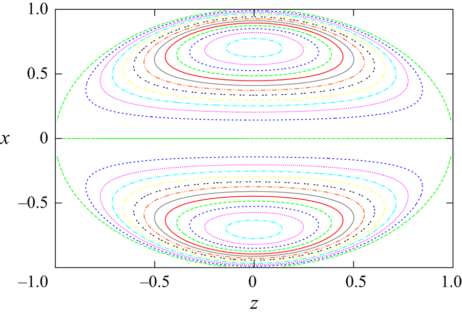
Figure 3. Streamlines for Hill's spherical vortex (3.12) in the meridional plane  $y=0$ with the $z$-axis being the axis of rotation.
3.1. Introduction
In this subsection, we will describe the mathematical model for Hill's spherical vortex. In order to avoid an excessive number of suffices, the same notation as in § 2 will be used for a number of the quantities; these are defined anew in this section. We adopt a spherical polar coordinate system in which  $r \leq R$ is the radial coordinate, $\theta$ is the polar angle and $R$ is the radius of a sphere. The radial and polar coordinates of velocity are given by $u$ and $v$, respectively. We denote the pressure by $p$ and the vorticity $\omega$ by
 \begin{equation} \omega = \frac{1}{r} \frac{\partial}{\partial r} (r v) - \frac{1}{r} \frac{\partial u}{\partial \theta}. \end{equation}
The axisymmetric continuity and Navier–Stokes equations for incompressible Newtonian fluids in spherical polar coordinates become
 \begin{gather} \frac{1}{r^2} \frac{\partial}{\partial r}(r^2 u) + \frac{1}{r \sin(\theta)} \frac{\partial}{\partial \theta}(v \sin(\theta)) = 0, \end{gather}
 \begin{gather} u \frac{\partial u}{\partial r} + \frac{v}{r} \frac{\partial u}{\partial \theta} -\frac{v^2}{r} +\frac{\partial p}{\partial r} ={-}\frac{\epsilon}{r \sin (\theta)} \frac{\partial}{\partial \theta} (\sin(\theta) \omega) , \end{gather}
 \begin{gather} u \frac{\partial v}{\partial r} + \frac{v}{r} \frac{\partial v}{\partial \theta} +\frac{uv}{r} +\frac{1}{r} \frac{\partial p}{\partial \theta} = \frac{\epsilon}{r} \frac{\partial}{\partial r} (r \omega) , \end{gather}
where  $\epsilon =1/ Re$ is the reciprocal of the Reynolds number and $0 < \epsilon \ll 1$. The boundary conditions are
 \begin{equation} u(R,\theta) = 0, \quad v(R, \theta) = C \sin ( \theta ), \end{equation}
in which  $C$ is a negative constant. Hill's spherical vortex corresponds to $C = - 3 U / 2$, where $U$ is the far-field velocity of the surrounding flow.
3.2. The leading-order solution
We will first perform the perturbation procedure on the nonlinear system (3.3)–(3.4a,b) and obtain the solution for Hill's spherical vortex. We introduce expansions of the form
 \begin{equation} u \sim u_0 + \epsilon u_1, \quad v \sim v_0 + \epsilon v_1, \quad p \sim p_0 + \epsilon p_1 , \quad \omega \sim \omega_0 + \epsilon \omega_1 , \end{equation}
as  $\epsilon \rightarrow 0$. At leading order, we obtain
 $$\begin{gather} \bar{L} u_0 - \frac{v_0^2}{r} +\frac{\partial p_0}{\partial r} = 0, \end{gather}$$
 $$\begin{gather}\bar{L} v_0 + \frac{u_0 v_0}{r} +\frac{1}{r} \frac{\partial p_0}{\partial \theta} = 0, \end{gather}$$
 $$\begin{gather}\frac{1}{r^2} \frac{\partial}{\partial r}(r^2 u_0) + \frac{1}{r \sin(\theta)} \frac{\partial}{\partial \theta}(v_0 \sin(\theta)) = 0, \end{gather}$$
with the differential operator
 \begin{equation} \bar{L}= u_0 \frac{\partial}{\partial r} + \frac{v_0}{r} \frac{\partial}{\partial \theta} \end{equation}
and the boundary conditions
 \begin{equation} u_0(R,\theta) = 0, \quad v_0(R, \theta) = C \sin ( \theta ). \end{equation}
Using (3.6a)–(3.6b), the vorticity equation becomes  $\bar {L} (\omega _0 / r \sin (\theta ) ) = 0$. Henceforth, we assume a solution of this equation of the form $\omega _0 = \alpha r \sin (\theta )$, where $\alpha$ is a constant to be determined shortly. The Stokes streamfunction is defined by
 \begin{equation} u_0 = \frac{1}{r^2 \sin (\theta)} \frac{\partial \psi}{\partial \theta}, \quad v_0 ={-} \frac{1}{r \sin (\theta)} \frac{\partial \psi}{\partial r}, \end{equation}
so that (3.6c) is automatically satisfied. The streamfunction  $\psi$ satisfies the following partial differential equation
 \begin{equation} \frac{\partial^2 \psi}{\partial r^2} + \frac{\sin(\theta)}{r^2} \frac{\partial}{\partial \theta} \left [ \frac{1}{\sin(\theta)} \frac{\partial \psi}{\partial \theta} \right ] ={-} \alpha r^2 \sin^2 (\theta) \end{equation}
for  $r < R$ with the boundary conditions
 \begin{equation} \psi (R,\theta) = 0, \quad \frac{\partial \psi}{\partial r} (R,\theta) ={-}C R \sin^2 ( \theta). \end{equation}
Hill's spherical vortex corresponds to the solution of this problem in the form
 \begin{equation} \psi (r, \theta) = \frac{C r^2}{2} \left ( 1 - \frac{r^2}{R^2} \right ) \sin^2 (\theta) \end{equation}
for  $r \leq R$ and provided that $\alpha = 5 C / R^2$. The streamlines for $C=-1$ and $R=1$ are shown in figure 3. We deduce that the velocities are
 \begin{equation} u_0 = C \left ( 1 - \frac{r^2}{R^2} \right ) \cos (\theta), \quad v_0 ={-}C \left ( 1 - \frac{2 r^2}{R^2} \right ) \sin (\theta). \end{equation}
3.3. The first correction
We now derive the linear problem for the first correction and the conditions (3.23) under which it may have a solution. At next order, we obtain
 \begin{equation} L \boldsymbol{z} =
\left(\begin{array}{@{}c@{}} \displaystyle-\dfrac{1}{r \sin
(\theta)} \dfrac{\partial}{\partial \theta} (\sin(\theta)
\omega_0)\\[10pt] \displaystyle\dfrac{1}{r}
\dfrac{\partial}{\partial r} (r \omega_0)\\ 0
\end{array}\right), \end{equation}
\begin{equation} L \boldsymbol{z} =
\left(\begin{array}{@{}c@{}} \displaystyle-\dfrac{1}{r \sin
(\theta)} \dfrac{\partial}{\partial \theta} (\sin(\theta)
\omega_0)\\[10pt] \displaystyle\dfrac{1}{r}
\dfrac{\partial}{\partial r} (r \omega_0)\\ 0
\end{array}\right), \end{equation}
in which
 \begin{equation}
L=\left(\begin{array}{@{}ccc@{}} \displaystyle \bar{L} +
\dfrac{\partial u_0}{\partial r} & \displaystyle
\dfrac{1}{r} \dfrac{\partial u_0}{\partial \theta} -
\dfrac{2 v_0}{r} & \displaystyle \dfrac{\partial}{\partial
r}\\[10pt] \displaystyle \dfrac{1}{r}
\dfrac{\partial}{\partial r} (r v_0) & \displaystyle
\bar{L} + \dfrac{1}{r} \dfrac{\partial v_0}{\partial
\theta} + \dfrac{u_0}{r} & \displaystyle \dfrac{1}{r}
\dfrac{\partial}{\partial \theta}\\[10pt] \displaystyle
\dfrac{\partial}{\partial r} + \dfrac{2}{r} & \displaystyle
\dfrac{1}{r} \dfrac{\partial}{\partial \theta}+
\dfrac{\cot(\theta)}{r} & \displaystyle 0
\end{array}\right), \quad
\boldsymbol{z}=\left(\begin{array}{@{}c@{}} u_1\\ v_1\\ p_1
\end{array}\right),
\end{equation}
\begin{equation}
L=\left(\begin{array}{@{}ccc@{}} \displaystyle \bar{L} +
\dfrac{\partial u_0}{\partial r} & \displaystyle
\dfrac{1}{r} \dfrac{\partial u_0}{\partial \theta} -
\dfrac{2 v_0}{r} & \displaystyle \dfrac{\partial}{\partial
r}\\[10pt] \displaystyle \dfrac{1}{r}
\dfrac{\partial}{\partial r} (r v_0) & \displaystyle
\bar{L} + \dfrac{1}{r} \dfrac{\partial v_0}{\partial
\theta} + \dfrac{u_0}{r} & \displaystyle \dfrac{1}{r}
\dfrac{\partial}{\partial \theta}\\[10pt] \displaystyle
\dfrac{\partial}{\partial r} + \dfrac{2}{r} & \displaystyle
\dfrac{1}{r} \dfrac{\partial}{\partial \theta}+
\dfrac{\cot(\theta)}{r} & \displaystyle 0
\end{array}\right), \quad
\boldsymbol{z}=\left(\begin{array}{@{}c@{}} u_1\\ v_1\\ p_1
\end{array}\right),
\end{equation}
with the boundary conditions
 \begin{equation} u_1 (R,\theta) = 0, \quad v_1 (R, \theta) = 0. \end{equation}
Saffman (Reference Saffman1992) stated one solution to the linear problem for the first correction (3.14)–(3.16a,b). By the Fredholm alternative, there is either a unique solution or an infinite number of solutions. We study the adjoint problem to check our approach and to establish how many solutions exist to this important problem. Following a modified version of the analysis in Smith (Reference Smith2010), we have an equation with the right-hand side in divergence form
 \begin{align} \boldsymbol{r}^T L \boldsymbol{z} - \boldsymbol{z}^T L^* \boldsymbol{r}&= \frac{1}{r^2} \frac{\partial}{\partial r} [ r^2 u_0 \{ a u_1 + b v_1 \} +r^2 a p_1 +r^2 c u_1 ] \nonumber\\ &\quad +\frac{1}{r \sin(\theta)} \frac{\partial}{\partial \theta} [ \sin(\theta) ( v_0 \{ a u_1 + b v_1 \} + b p_1 + c v_1 )], \end{align}
in which the adjoint operator  $L^*$ and vector $\boldsymbol {r}$ are given by
 \begin{equation} L^{*}=\left(\begin{array}{ccc} \displaystyle -\bar{L} + \dfrac{\partial u_0}{\partial r} & \displaystyle \dfrac{1}{r} \dfrac{\partial}{\partial r} (r v_0) & \displaystyle -\dfrac{\partial}{\partial r}\\[8pt] \displaystyle \dfrac{1}{r} \dfrac{\partial u_0}{\partial \theta} - \dfrac{2 v_0}{r} & \displaystyle -\bar{L} + \dfrac{1}{r} \dfrac{\partial v_0}{\partial \theta} + \dfrac{u_0}{r} & \displaystyle -\dfrac{1}{r} \dfrac{\partial}{\partial \theta}\\[8pt] \displaystyle -\dfrac{\partial}{\partial r} - \dfrac{2}{r} & \displaystyle - \dfrac{1}{r} \dfrac{\partial}{\partial \theta} - \dfrac{\cot (\theta)}{r} & \displaystyle 0 \end{array}\right),\quad \boldsymbol{r}=\left(\begin{array}{c} a\\ b\\ c \end{array}\right). \end{equation}
Equation (3.17) may be integrated to yield
 \begin{equation} \langle \boldsymbol{r}^T L \boldsymbol{z} - \boldsymbol{z}^T L^* \boldsymbol{r} \rangle = 0, \end{equation}
where
 \begin{equation} \langle \ {\bullet}\ \rangle = \int^{\rm \pi}_{\theta=0} \int^{R}_{r=0} \ {\bullet}\ r^2 \sin(\theta) \,\textrm{d} r \,\textrm{d} \theta, \end{equation}
provided that the following condition is satisfied on the boundary of the sphere:
 \begin{equation} a(R, \theta) = 0. \end{equation}
It follows from this that if
 \begin{equation} L^* \boldsymbol{r} = \boldsymbol{0}, \end{equation}
subject to the condition (3.21), then our linear problem for the first correction (3.14)–(3.16a,b) can only have a solution if
 \begin{equation} \left \langle - \frac{a}{r \sin(\theta)} \frac{\partial}{\partial \theta} (\sin(\theta) \omega_0) + \frac{b}{r} \frac{\partial}{\partial r} (r \omega_0) \right \rangle=0, \end{equation}
for any  $\boldsymbol {r}=(a,b,c)^\textrm {T}$ in the null space of the adjoint problem. It remains to find the linearly independent solution vectors $\boldsymbol {r}$ and substitute them into (3.23).
A linearly independent solution of the adjoint problem (3.22) and (3.21) is
 \begin{equation} \boldsymbol{r}_1 = (0,0,1)^\textrm{T}. \end{equation}
An infinite family of linearly independent solutions is given by
 \begin{equation} \boldsymbol{r}_2 = \left(f(\psi) u_0, f(\psi) v_0, -\alpha \int^{\psi} f(s) \, \textrm{d} s \right)^\textrm{T}. \end{equation}
The function  $f(\psi )$ is differentiable on the domain $[C R^2 / 8, 0]$. Given this condition, the Weierstrass approximation theorem ensures that a polynomial,
 \begin{equation} p(\psi) = a_0 + a_1 \psi + \cdots + a_q \psi^q, \end{equation}
exists with  $a_i$ real constants and $q$ non-negative integer which uniformly approximates $f(\psi )$ on the domain $[C R^2 / 8,0]$. We consider the vector space of polynomials $p(\psi )$ over the field of real numbers. If we construct a basis for this space of polynomials $\{ \psi ^n \mid n \in \textrm {I N} \cup \{ 0 \} \}$, then all functions $f(\psi )$ are uniformly approximated by our basis. Hence, it is sufficient to construct solvability conditions for the basis. A countably infinite family of linearly independent solutions of the adjoint problem (2.29) and (2.28) have been deduced; that is, $f(\psi )=\psi ^n$ for $n$ in the non-negative integers.
A family of vorticity equations are required for Stuart cats’ eyes, Mallier–Maslowe vortices, travelling waves in two-dimensional plane Poiseuille flow (Smith & Wissink Reference Smith and Wissink2015) and two-dimensional Kolmogorov flow (Smith & Wissink Reference Smith and Wissink2018). However, in the case of Hill's spherical vortex, there are no solutions corresponding to vorticity.
3.4. Solvability conditions
Only the second solution corresponds to physical solvability conditions. The corresponding solvability conditions are
 \begin{equation} \left \langle - \frac{\psi^{n} u_0}{r \sin(\theta)} \frac{\partial}{\partial \theta} (\sin(\theta) \omega_0) + \frac{\psi^{n} v_0}{r} \frac{\partial}{\partial r} (r \omega_0) \right \rangle=0, \end{equation}
where  $n$ is a non-negative integer. In the remainder of this subsection, the leading-order solution will be shown to satisfy this countably infinite set of solvability conditions.
We substitute the leading-order solution (3.12)–(3.13a,b) into the left-hand side of the solvability conditions (3.27) to yield
 \begin{align} &\left \langle - \frac{\psi^{n} u_0}{r \sin(\theta)} \frac{\partial}{\partial \theta} (\sin(\theta) \omega_0) + \frac{\psi^{n} v_0}{r} \frac{\partial}{\partial r} (r \omega_0)\right \rangle \nonumber\\ &\quad ={-}\frac{40}{R^2} \left ( \frac{C}{2} \right )^{n+2} \int^{R}_{r=0} r^{2n+2} \left ( 1 - \frac{r^2}{R^2} \right )^{n+1} \textrm{d} r \int^{\rm \pi}_{\theta=0} \sin^{2 n + 1}(\theta) \cos^2 (\theta) \,\textrm{d} \theta \nonumber\\ &\qquad -\frac{40}{R^2} \left ( \frac{C}{2} \right )^{n+2} \int^{R}_{r=0} r^{2n+2} \left ( 1 - \frac{r^2}{R^2} \right )^{n} \left ( 1 - \frac{2 r^2}{R^2} \right ) \textrm{d} r \int^{\rm \pi}_{\theta=0} \sin^{2 n + 3}(\theta) \,\textrm{d} \theta. \end{align}
The second term on the right-hand side may be rewritten
 \begin{align} &\left \langle - \frac{\psi^{n} u_0}{r \sin(\theta)} \frac{\partial}{\partial \theta} (\sin(\theta) \omega_0) + \frac{\psi^{n} v_0}{r} \frac{\partial}{\partial r} (r \omega_0) \right \rangle \nonumber\\ &\quad ={-}\frac{40}{R^2} \left ( \frac{C}{2} \right )^{n+2} \int^{R}_{r=0} r^{2n+2} \left ( 1 - \frac{r^2}{R^2} \right )^{n+1} \textrm{d} r \int^{\rm \pi}_{\theta=0} \sin^{2 n + 1}(\theta) \cos^2 (\theta) \,\textrm{d} \theta \nonumber\\ &\qquad -\frac{40}{R^2} \left ( \frac{C}{2} \right )^{n+2} \int^{R}_{r=0} r^{2n + 2} \left ( 1 - \frac{r^2}{R^2} \right )^{n+1} \textrm{d} r \int^{\rm \pi}_{\theta=0} \sin^{2 n + 3}(\theta) \,\textrm{d} \theta\nonumber\\ &\qquad +\frac{40}{R^4} \left ( \frac{C}{2} \right )^{n+2} \int^{R}_{r=0} r^{2(n+2)} \left ( 1 - \frac{r^2}{R^2} \right )^{n} \textrm{d} r \int^{\rm \pi}_{\theta=0} \sin^{2 n + 3}(\theta) \,\textrm{d} \theta. \end{align}
Using the two identities involving definite integrals in Appendix A, we find that
 \begin{align} &\left \langle - \frac{\psi^{n} u_0}{r \sin(\theta)} \frac{\partial}{\partial \theta} (\sin(\theta) \omega_0) + \frac{\psi^{n} v_0}{r} \frac{\partial}{\partial r} (r \omega_0)\right \rangle \nonumber\\ &\quad ={-}\frac{40}{R^2} \left ( \frac{C}{2} \right )^{n+2} \int^{\rm \pi}_{\theta=0} \sin^{2 n + 1}(\theta) \,\textrm{d} \theta \nonumber\\ &\qquad \times\left \{ \int^{R}_{r=0} r^{2n + 2} \left ( 1 - \frac{r^2}{R^2} \right )^{n+1} \textrm{d} r - \frac{2 n + 2}{(2 n + 3)} \frac{1}{R^2} \int^{R}_{r=0} r^{2(n+2)} \left ( 1 - \frac{r^2}{R^2} \right )^{n} \textrm{d} r \right \}. \end{align}
If we apply integration by parts to the first of the two integrals in the curly brackets, then the first integral is shown to be equal and opposite to the second integral. Therefore, all of the solvability conditions are satisfied. Provided that there are no further solutions to the adjoint problem (3.21)–(3.22), the problem for the first correction (3.14)–(3.16a,b) does have an infinite family of solutions by the Fredholm alternative. In fact, one member of this infinite family of solutions of (3.14)–(3.16a,b) is given by  $u_1=v_1=0$ and $p_1=-2 \alpha r \cos (\theta )$, which was described by Saffman (Reference Saffman1992). Hill's spherical vortex has been confirmed to be consistent with the Navier–Stokes equations. We now consider a graphical interpretation in the case of Hill's spherical vortex. Equations (3.27) represent a manifold in infinite-dimensional phase space for steady states of the Navier–Stokes equations, which is denoted by an (orange) surface in figure 4. The leading-order solution (3.12) is represented by a (green) dot in figure 4, which resides on the manifold. In the case of Stuart cats’ eyes or the Mallier–Maslowe vortices, the manifold is given by the steady version of (2.38)–(2.40) and the leading-order solutions are (2.13) and (2.18), respectively. However, these leading-order solutions are now represented by the (red) cross in figure 4, which do not reside on the appropriate manifold.
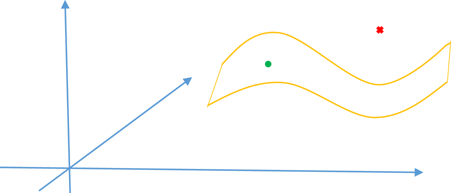
Figure 4. A schematic of the structure of infinite-dimensional phase space for steady states of the Navier–Stokes equations. The (orange) surface denotes the viscous manifold for asymptotic solutions of the Navier–Stokes equations in the high-Reynolds-number limit. The (green) dot represents the leading-order solution in the case of Hill's spherical vortex and the (red) cross represents the leading-order solution for either the Stuart cats’ eyes or the Mallier–Maslowe vortices.
4. Lamb–Chaplygin dipole
The Lamb–Chaplygin dipole (Lamb Reference Lamb1895; Chaplygin Reference Chaplygin1903) describes a dipolar vortex structure within a circle of constant radius. When placed in an irrotational flow, this dipole will propagate without deformation and at a constant flow speed through the fluid. It is a planar solution to the Euler equations with its streamlines being illustrated in figure 5. The Lamb–Chaplygin dipole has been applied to analyse the dynamics of vortices in atmospheric and oceanographic flows (Billant & Chomaz Reference Billant and Chomaz2000; Suzuki, Hirota & Hattori Reference Suzuki, Hirota and Hattori2018). In this section, we will investigate whether or not the Lamb–Chaplygin dipole approximates a steady state or quasi-steady state of the Navier–Stokes equations.
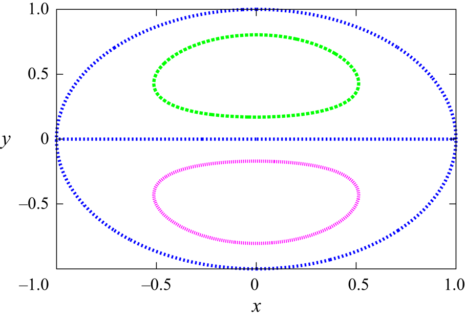
Figure 5. Streamlines for the Lamb–Chaplygin dipole (4.13).
4.1. Introduction
In this subsection, we will describe the mathematical model for the Lamb–Chaplygin dipole. In order to avoid an excessive number of suffices, the same notation as in §§ 2 and 3 will be adopted for a number of the quantities; these are defined anew in this section. The system of dimensionless equations to be studied are now introduced. We consider the two-dimensional Navier–Stokes equations for incompressible Newtonian fluids in plane polar coordinates
 $$\begin{gather} \frac{\partial u}{\partial t} + u \frac{\partial u}{\partial r} + \frac{v}{r} \frac{\partial u}{\partial \theta} -\frac{v^2}{r} +\frac{\partial p}{\partial r} ={-} \frac{\epsilon}{r} \frac{\partial \omega}{\partial \theta}, \end{gather}$$
 $$\begin{gather}\frac{\partial v}{\partial t} + u \frac{\partial v}{\partial r} + \frac{v}{r} \frac{\partial v}{\partial \theta} +\frac{uv}{r} +\frac{1}{r} \frac{\partial p}{\partial \theta} = \epsilon \frac{\partial \omega}{\partial r}, \end{gather}$$
and the continuity equation of the form
 \begin{equation} \frac{1}{r} \frac{\partial}{\partial r}(ru) + \frac{1}{r} \frac{\partial v}{\partial \theta} = 0, \end{equation}
in which  $r < R$ is the radial coordinate, $R$ is the radius of the circle, $\theta$ is the azimuthal coordinate, $t$ is time, $u$ is the radial velocity component, $v$ is the azimuthal velocity component, $p$ is the pressure, $\omega$ is the vorticity given by
 \begin{equation} {\omega} = \frac{1}{r} \frac{\partial}{\partial r}(r v)- \frac{1}{r} \frac{\partial u}{\partial \theta}, \end{equation} $\epsilon = 1/ Re$ is the reciprocal of the Reynolds number and $0 < \epsilon \ll 1$. The boundary conditions are
 \begin{equation} \left.\begin{array}{c@{}}
u(R,\theta,t) = 0, \quad v(R, \theta,t) = C (\epsilon t)
\sin ( \theta ), \\[4pt] {[}u,v,p](r,0,t)=[u,v,p](r,2 {\rm \pi}, t),
\end{array}\right\} \end{equation}
\begin{equation} \left.\begin{array}{c@{}}
u(R,\theta,t) = 0, \quad v(R, \theta,t) = C (\epsilon t)
\sin ( \theta ), \\[4pt] {[}u,v,p](r,0,t)=[u,v,p](r,2 {\rm \pi}, t),
\end{array}\right\} \end{equation}
in which  $C (\epsilon t)$ is a non-zero slowly varying function. The Lamb–Chaplygin dipole corresponds to $C = - 2 U$, where $U$ is the far-field velocity of the surrounding flow.
4.2. The leading-order solution
We will first perform the perturbation procedure on the nonlinear system (4.1)–(4.4) and obtain the solution for Lamb–Chaplygin dipole. We introduce expansions of the form
 \begin{equation} u \sim u_0 + \epsilon u_1, \quad v \sim v_0 + \epsilon v_1, \quad p \sim p_0 + \epsilon p_1 , \quad \omega \sim \omega_0 + \epsilon \omega_1 , \end{equation}
as  $\epsilon \rightarrow 0$. At leading order, for the quasi-steady state, we obtain
 $$\begin{gather} \bar{L} u_0 - \frac{v_0^2}{r} + \frac{\partial p_0}{\partial r} = 0, \end{gather}$$
 $$\begin{gather}\bar{L} v_0 + \frac{u_0 v_0}{r} + \frac{1}{r} \frac{\partial p_0}{\partial \theta} = 0, \end{gather}$$
 $$\begin{gather}\frac{1}{r} \frac{\partial}{\partial r}(ru_0) + \frac{1}{r} \frac{\partial v_0}{\partial \theta} = 0, \end{gather}$$
where the differential operator
 \begin{equation} \bar{L}=u_0 \frac{\partial}{\partial r} + \frac{1}{r} v_0 \frac{\partial}{\partial \theta}. \end{equation}
We take the radial partial derivative of (4.6b) in the form
 \begin{equation} u_0 \frac{\partial}{\partial r} (r v_0) + v_0 \frac{\partial v_0}{\partial \theta} + \frac{\partial p_0}{\partial \theta} = 0 \end{equation}
minus the azimuthal partial derivative of (4.6a) to obtain the vorticity equation  $\bar {L} \omega _0 =0$. A streamfunction $\psi$ is defined by the equations
 \begin{equation} u_0 = \frac{1}{r} \frac{\partial \psi}{\partial \theta}, \quad v_0 ={-} \frac{\partial \psi}{\partial r}, \end{equation}
so that (4.6c) is automatically satisfied and the vorticity equation may be rewritten as
 \begin{equation} \frac{\partial \psi}{\partial \theta} \frac{\partial \omega_0}{\partial r} -\frac{\partial \psi}{\partial r} \frac{\partial \omega_0}{\partial \theta}=0. \end{equation}
The Lamb–Chaplygin dipole corresponds to the solution of (4.10) given by  $\omega _0 = k^2 \psi$ with k being an arbitrary constant, so that $\psi$ satisfies the partial differential equation
 \begin{equation} \frac{\partial^2 \psi}{\partial r^2} + \frac{1}{r} \frac{\partial \psi}{\partial r} + \frac{1}{r^2} \frac{\partial^2 \psi}{\partial \theta^2} ={-}k^2 \psi \end{equation}
for  $r < R$ with the boundary conditions
 \begin{equation} \psi (R,\theta, \tilde{t}) = 0, \quad \frac{\partial \psi}{\partial r} (R,\theta, \tilde{t}) ={-}C (\tilde{t}) \sin ( \theta), \quad \psi(r,0, \tilde{t})=\psi(r,2 {\rm \pi}, \tilde{t}), \end{equation}
in which  $\tilde {t} =\epsilon t$ is the slowly varying time scale. The Lamb–Chaplygin dipole corresponds to the solution of this boundary value problem in the form
 \begin{equation} \psi (r, \theta, \tilde{t}) ={-}\frac{C (\tilde{t}) J_1 (k r) \sin (\theta)}{k J_0(k R)}, \end{equation}
for  $r \leq R$. The first zero of the Bessel function $J_1 (k R)=0$ fixes $k R \approx 3.8317$. The streamlines for $C (\tilde {t})=1$ and $R=1$ are shown in figure 5. We deduce that the velocities are given by
 \begin{equation} u_0 (r, \theta, \tilde{t}) ={-}\frac{C (\tilde{t}) J_1 (k r) \cos (\theta)}{k r J_0(k R)}, \quad v_0 (r, \theta, \tilde{t}) = \frac{C (\tilde{t}) J_1^{\prime} (k r) \sin (\theta)}{J_0(k R)}. \end{equation}
4.3. The first correction
We now derive the linear problem for the first correction and the conditions (4.24) under which it may have a solution. At next order, we obtain
 \begin{equation} L \boldsymbol{z} =
\left(\begin{array}{@{}c@{}} \displaystyle -\dfrac{\partial
u_0}{\partial \tilde{t}} - \dfrac{1}{r} \dfrac{\partial
\omega_0}{\partial \theta}\\[10pt] \displaystyle
-\dfrac{\partial v_0}{\partial \tilde{t}} + \dfrac{\partial
\omega_0}{\partial r}\\ 0
\end{array}\right)=\left(\begin{array}{@{}c@{}}
\displaystyle -\dfrac{\partial u_0}{\partial \tilde{t}} -
k^2 u_0\\[10pt] \displaystyle -\dfrac{\partial v_0}{\partial
\tilde{t}} - k^2 v_0\\ 0 \end{array} \right),
\end{equation}
\begin{equation} L \boldsymbol{z} =
\left(\begin{array}{@{}c@{}} \displaystyle -\dfrac{\partial
u_0}{\partial \tilde{t}} - \dfrac{1}{r} \dfrac{\partial
\omega_0}{\partial \theta}\\[10pt] \displaystyle
-\dfrac{\partial v_0}{\partial \tilde{t}} + \dfrac{\partial
\omega_0}{\partial r}\\ 0
\end{array}\right)=\left(\begin{array}{@{}c@{}}
\displaystyle -\dfrac{\partial u_0}{\partial \tilde{t}} -
k^2 u_0\\[10pt] \displaystyle -\dfrac{\partial v_0}{\partial
\tilde{t}} - k^2 v_0\\ 0 \end{array} \right),
\end{equation}
in which
 \begin{equation}
L=\left(\begin{array}{@{}ccc@{}} \displaystyle \bar{L} +
\dfrac{\partial u_0}{\partial r} & \displaystyle
\dfrac{1}{r} \dfrac{\partial u_0}{\partial \theta} -
\dfrac{2 v_0}{r} & \displaystyle \dfrac{\partial}{\partial
r}\\[10pt] \displaystyle \dfrac{1}{r}
\dfrac{\partial}{\partial r} (r v_0) & \displaystyle
\bar{L} + \dfrac{1}{r} \dfrac{\partial v_0}{\partial
\theta} + \dfrac{u_0}{r} & \displaystyle \dfrac{1}{r}
\dfrac{\partial}{\partial \theta}\\[10pt] \displaystyle
\dfrac{\partial}{\partial r} + \dfrac{1}{r} & \displaystyle
\dfrac{1}{r} \dfrac{\partial}{\partial \theta} &
\displaystyle 0 \end{array}\right),\quad
\boldsymbol{z}=\left(\begin{array}{@{}c@{}} u_1\\ v_1\\ p_1
\end{array}\right), \end{equation}
\begin{equation}
L=\left(\begin{array}{@{}ccc@{}} \displaystyle \bar{L} +
\dfrac{\partial u_0}{\partial r} & \displaystyle
\dfrac{1}{r} \dfrac{\partial u_0}{\partial \theta} -
\dfrac{2 v_0}{r} & \displaystyle \dfrac{\partial}{\partial
r}\\[10pt] \displaystyle \dfrac{1}{r}
\dfrac{\partial}{\partial r} (r v_0) & \displaystyle
\bar{L} + \dfrac{1}{r} \dfrac{\partial v_0}{\partial
\theta} + \dfrac{u_0}{r} & \displaystyle \dfrac{1}{r}
\dfrac{\partial}{\partial \theta}\\[10pt] \displaystyle
\dfrac{\partial}{\partial r} + \dfrac{1}{r} & \displaystyle
\dfrac{1}{r} \dfrac{\partial}{\partial \theta} &
\displaystyle 0 \end{array}\right),\quad
\boldsymbol{z}=\left(\begin{array}{@{}c@{}} u_1\\ v_1\\ p_1
\end{array}\right), \end{equation}
with the boundary conditions
 \begin{equation} \left.\begin{array}{c@{}}
u_1 (R,\theta, \tilde{t}) = 0, \quad v_1 (R, \theta,
\tilde{t}) = 0, \\[4pt] {[}u_1,v_1,p_1](r,0,
\tilde{t})=[u_1,v_1,p_1](r,2 {\rm \pi}, \tilde{t}).
\end{array}\right\} \end{equation}
\begin{equation} \left.\begin{array}{c@{}}
u_1 (R,\theta, \tilde{t}) = 0, \quad v_1 (R, \theta,
\tilde{t}) = 0, \\[4pt] {[}u_1,v_1,p_1](r,0,
\tilde{t})=[u_1,v_1,p_1](r,2 {\rm \pi}, \tilde{t}).
\end{array}\right\} \end{equation}
A general solution to the linear problem for the first correction (4.15)–(4.17) is very difficult to find. Therefore, we study the adjoint problem in order to determine the conditions under which the problem for the first correction has a solution. Following a modified version of the analysis in Smith (Reference Smith2007), we have the following divergence formulation:
 \begin{align} \boldsymbol{r}^T L \boldsymbol{z} - \boldsymbol{z}^T L^* \boldsymbol{r}&= \frac{1}{r} \frac{\partial}{\partial r} \left[ r u_0 \{ a u_1 + b v_1 \} +r a p_1 +r c u_1 \right] \nonumber\\ &\quad +\frac{1}{r} \frac{\partial}{\partial \theta} \left[ v_0 \{ a u_1 + b v_1 \} + b p_1 + c v_1 \right], \end{align}
in which the adjoint operator  $L^*$ and vector $\boldsymbol {r}$ are given by
 \begin{equation}
L^{*}=\left(\begin{array}{@{}ccc@{}} \displaystyle -\bar{L} +
\dfrac{\partial u_0}{\partial r} & \displaystyle
\dfrac{1}{r} \dfrac{\partial}{\partial r} (r v_0) &
\displaystyle -\dfrac{\partial}{\partial r}\\[10pt]
\displaystyle \dfrac{1}{r} \dfrac{\partial u_0}{\partial
\theta} - \dfrac{2 v_0}{r} & \displaystyle -\bar{L} +
\dfrac{1}{r} \dfrac{\partial v_0}{\partial \theta} +
\dfrac{u_0}{r} & \displaystyle -\dfrac{1}{r}
\dfrac{\partial}{\partial \theta}\\[10pt] \displaystyle
-\dfrac{\partial}{\partial r} - \dfrac{1}{r} &
\displaystyle - \dfrac{1}{r} \dfrac{\partial}{\partial
\theta} & \displaystyle 0 \end{array}\right),
\quad \boldsymbol{r}=\left(\begin{array}{@{}c@{}} a\\ b\\ c
\end{array}\right). \end{equation}
\begin{equation}
L^{*}=\left(\begin{array}{@{}ccc@{}} \displaystyle -\bar{L} +
\dfrac{\partial u_0}{\partial r} & \displaystyle
\dfrac{1}{r} \dfrac{\partial}{\partial r} (r v_0) &
\displaystyle -\dfrac{\partial}{\partial r}\\[10pt]
\displaystyle \dfrac{1}{r} \dfrac{\partial u_0}{\partial
\theta} - \dfrac{2 v_0}{r} & \displaystyle -\bar{L} +
\dfrac{1}{r} \dfrac{\partial v_0}{\partial \theta} +
\dfrac{u_0}{r} & \displaystyle -\dfrac{1}{r}
\dfrac{\partial}{\partial \theta}\\[10pt] \displaystyle
-\dfrac{\partial}{\partial r} - \dfrac{1}{r} &
\displaystyle - \dfrac{1}{r} \dfrac{\partial}{\partial
\theta} & \displaystyle 0 \end{array}\right),
\quad \boldsymbol{r}=\left(\begin{array}{@{}c@{}} a\\ b\\ c
\end{array}\right). \end{equation}
Equation (4.18) may be integrated to yield
 \begin{equation} \langle \boldsymbol{r}^T L \boldsymbol{z} - \boldsymbol{z}^T L^* \boldsymbol{r} \rangle = 0, \end{equation}
where
 \begin{equation} \langle \ {\bullet} \ \rangle = \int^{2 {\rm \pi}}_{\theta=0} \int^{R}_{r=0}\ {\bullet} \ r \,\textrm{d} r \,\textrm{d} \theta, \end{equation}
provided that the following periodicity conditions and boundary condition on the radius of the circle are satisfied:
 $$\begin{gather} [a,b,c](r,0, \tilde{t}) = [a,b,c](r,2 {\rm \pi}, \tilde{t}), \end{gather}$$
 $$\begin{gather}a(R, \theta, \tilde{t}) = 0. \end{gather}$$
It follows from this that if
 \begin{equation} L^* \boldsymbol{r} = \boldsymbol{0}, \end{equation}
subject to the conditions (4.22), then our linear problem for the first correction (4.15)–(4.17) can only have a solution if
 \begin{equation} \left \langle a \left [ -\frac{\partial u_0}{\partial \tilde{t}} - k^2 u_0 \right ] + b \left [ -\frac{\partial v_0}{\partial \tilde{t}} - k^2 v_0 \right ] \right \rangle=0, \end{equation}
for any  $\boldsymbol {r}=(a,b,c)^\textrm {T}$ in the null space of the adjoint problem. It remains to find the linearly independent solution vectors $\boldsymbol {r}$ and substitute them into (4.24).
Two linearly independent solutions of the adjoint problem (4.23) and (4.22) are
 \begin{equation} \boldsymbol{r}_1 = (0, 0, 1)^\textrm{T}, \quad \boldsymbol{r}_2 = (0,r,r v_0)^\textrm{T}. \end{equation}
An infinite family of linearly independent solutions is given by
 \begin{equation} \boldsymbol{r}_3 = \left(f(\psi) u_0, f(\psi) v_0, -k^2 \int^{\psi} sf(s) \, \textrm{d} s \right)^\textrm{T}. \end{equation}
The function  $f(\psi )$ is differentiable on $[-\psi _{max},\psi _{max}]$, where $\psi _{max}$ is the bound on the streamfunction. Given this condition, the Weierstrass approximation theorem ensures that a polynomial,
 \begin{equation} p(\psi) = a_0 + a_1 \psi + \cdots + a_q \psi^q, \end{equation}
exists with  $a_i$ real constants and $q$ non-negative integer which uniformly approximates $f(\psi )$ on $[-\psi _{max},\psi _{max}]$. We consider the vector space of polynomials $p(\psi )$ over the field of real numbers. If we construct a basis for this space of polynomials $\{ \psi ^n \mid n \in \textrm {I N} \cup \{ 0 \} \}$, then all functions $f(\psi )$ are uniformly approximated by our basis. Hence, it is sufficient to construct solvability conditions for the basis. A countably infinite family of linearly independent solutions of the adjoint problem (4.23) and (4.22) have been deduced; that is, $f(\psi )=\psi ^n$ for $n$ in the non-negative integers. We note that there are no linearly independent solutions corresponding to vorticity.
4.4. Modulation equations
The first solution to the adjoint problem,  $\boldsymbol {r}_1$, corresponds to a trivial modulation equation. Only the second and third solutions correspond to physical modulation equations, which are described in the following subsections.
4.4.1. Angular momentum modulation equation
If we substitute the second vector  $\boldsymbol {r}_2$ into (4.24), then we obtain our first secularity condition
 \begin{equation} \left \langle -\frac{\partial}{\partial \tilde{t}} (r v_0) - k^2 r v_0 \right \rangle=0. \end{equation}
This may be rewritten as the modulation equation
 \begin{equation} \frac{\textrm{d} }{\textrm{d} \tilde{t}} \langle r v_0 \rangle ={-}k^2 \langle r v_0 \rangle. \end{equation}
4.4.2. Generalized energy modulation equations
If we substitute the third vector,  $\boldsymbol {r}_3$, into (4.24) with $f(\psi )=\psi ^n$, then we obtain the further secularity condition
 \begin{equation} \left \langle \psi^n u_0 \left [ -\frac{\partial u_0}{\partial \tilde{t}} - k^2 u_0 \right ] + \psi^n v_0 \left [ -\frac{\partial v_0}{\partial \tilde{t}} - k^2 v_0 \right ] \right \rangle=0. \end{equation}
This may be rewritten as
 \begin{equation} \left \langle \psi^n \left [ \frac{\partial E_0}{\partial \tilde{t}} + 2 k^2 E_0 \right ] \right \rangle=0, \end{equation}
for  $n$ in the non-negative integers.
4.5. Inconsistency of the steady state
Using (4.31) when  $n=0$, we have the solvability condition
 \begin{equation} \langle E_0 \rangle =0. \end{equation}
The left-hand side of this solvability condition is positive and the solvability condition is not satisfied. The problem for the first correction (4.15)–(4.17) does not have a solution by the Fredholm alternative. The Lamb–Chaplygin dipole is a solution to the steady Euler equations, but it is not a leading-order solution to the steady Navier–Stokes equation for high-Reynolds-number flows. As such, the Lamb–Chaplygin dipole does not approximate a steady state of the Navier–Stokes equations.
4.6. Consistency of the quasi-steady state
If we substitute the leading-order solution (4.13)–(4.14a,b) into (4.29), then we have a trivial identity. Substitution of the leading-order solution (4.13)–(4.14a,b) into (4.31) produces the equation
 \begin{equation} \left \langle \psi^n E_0 \left [ \frac{\textrm{d} }{\textrm{d} \tilde{t}}(C^2) + 2 k^2 C^2 \right ] \right \rangle=0, \end{equation}
for  $n$ in the non-negative integers. This may be rewritten as
 \begin{equation} \langle \psi^n E_0 \rangle \left [ \frac{\textrm{d} C}{\textrm{d} \tilde{t}} + k^2 C \right ]=0. \end{equation}
These modulation equations are all satisfied providing
 \begin{equation} C(\tilde{t}) = C_0 \,\textrm{e}^{- k^2 \tilde{t}}, \end{equation}
where  $C_0$ is a constant of integration. Provided that there are no further solutions to the adjoint problem (4.22)–(4.23), the problem for the first correction (4.15)–(4.17) does have an infinite family of solutions by the Fredholm alternative. In fact, one member of this infinite family of solutions of (4.15)–(4.17) is given by $u_1=v_1=p_1=0$. Furthermore, our leading-order solution turns out to be an exact solution of the Navier–Stokes equations as described below.
4.7. An exact solution
If we rewrite the leading-order solution (4.13)–(4.14a,b) in terms of the original dimensionless variables, we obtain
 $$\begin{gather} u (r, \theta, t) ={-}\frac{C_0 \,\textrm{e}^{- k^2 \epsilon t} J_1 (k r) \cos (\theta)}{k r J_0(k R)}, \quad v (r, \theta, t) = \frac{C_0 \,\textrm{e}^{- k^2 \epsilon t} J_1^{\prime} (k r) \sin (\theta)}{J_0(k R)}, \end{gather}$$
 $$\begin{gather}\omega (r, \theta, t) ={-}\frac{k^2 C_0 \,\textrm{e}^{- k^2 \epsilon t} J_1 (k r) \sin (\theta)}{k J_0(k R)}, \quad p (r, \theta, t) ={-}\frac{\omega^2}{2 k^2}- \frac{1}{2}(u^2+v^2), \end{gather}$$
for  $r \leq R$. This is an original exact solution of the Navier–Stokes equations (4.1)–(4.4) provided that $C (\epsilon t) = C_0 \,\textrm {e}^{- k^2 \epsilon t}$.
This exact solution can be seen to be one of the most important because it is time dependent; it has non-zero nonlinear convective terms; it is restricted to a finite domain; and it has a decay rate dependent on the dipole radius. We do not know of another exact solution with this combination of properties (Drazin & Riley Reference Drazin and Riley2006). Numerical and experimental evidence also exists which indicate that it is linearly stable (see Couder & Basdevant Reference Couder and Basdevant1986).
The decay rate may be written in the form
 \begin{equation} \left ( \frac{3.8317}{R} \right )^2 \epsilon. \end{equation}
The decay rate varies with the reciprocal of the Reynolds number,  $\epsilon = 1/ Re$, and with the reciprocal of the square of the dipole radius $R$ (see figure 6). The decay rate increases rapidly as the dipole radius decreases. If the dipole radius $R \ll \epsilon ^{1/2} = Re^{-1/2}$, then the dissipation is exponentially fast. If the dipole radius $R \sim \epsilon ^{1/2} = Re^{-1/2}$, then the exponential decay is order one. Larger values of the dipole radius, $R \gg \epsilon ^{1/2} = Re^{-1/2}$, result in an exponentially slow dissipation rate and the solution may easily be mistaken for a steady state.


The long time scale viscous evolution of symmetric two-dimensional dipoles has been studied elsewhere in which the domain of rotational flow was not restricted to a circle. Kizner, Khvoles & Kessler (Reference Kizner, Khvoles and Kessler2010) have shown that viscosity first takes the dipole to an intermediate asymptotic state and then slowly moves away. Kizner et al. (Reference Kizner, Khvoles and Kessler2010) claim that, in the limit of vanishing viscosity (large Reynolds number), a unique elliptical dipole solution is selected with a separatrix aspect ratio of  $1.037$. Our exact solution of the full Navier–Stokes equations has shown that there is an alternative evolution when the domain of rotational flow is restricted to a circle.
5. Conclusions
An asymptotic technique has been introduced to establish whether or not an exact inviscid steady state solution approximates the behaviour of a real viscous fluid at high Reynolds number. The viscous terms in the Navier–Stokes equations are much smaller than the terms in the Euler equations in this limit, but the small viscous terms have a cumulative effect. First, if an exact inviscid steady state is to approximate a viscous steady state, then solvability conditions for the amplitude must be satisfied. Second, if an exact inviscid steady state is to approximate a viscous quasi-steady state, then modulation equations for the amplitude envelope must be satisfied. The solvability conditions (modulation equations), which govern steady states (quasi-steady states), require a family of equations for generalized energy in addition to those already known for travelling and standing waves. These conditions are very restrictive. Therefore, the vast majority of rotational exact inviscid steady states do not approximate a real viscous flow.
Employing this new technique in singular perturbation theory, we have analysed four exact inviscid steady states, which are widely used in stability analysis of vortex flows. Stuart cats’ eyes and Mallier–Maslowe vortices have been shown to be neither approximate steady states nor quasi-steady states of the Navier–Stokes equations. Hill's spherical vortex has been confirmed to be a leading-order approximation to a steady state of the Navier–Stokes equations in the core spherical region. Contrary to expectations, the Lamb–Chaplygin dipole has been shown not to approximate a steady state of the Navier–Stokes equations in the core circular region. These results are summarized in table 1.
Table 1. Classification of exact inviscid solutions.
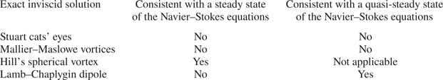
Couder & Basdevant (Reference Couder and Basdevant1986) have shown that the vortex profiles for the Lamb–Chaplygin dipole are in good agreement with numerical solutions of the two-dimensional Navier–Stokes equations. Our results have validated this well-established view (Wu et al. Reference Wu, Ma and Zhou2006). The Lamb–Chaplygin dipole is a leading-order approximation to a quasi-steady state of the Navier–Stokes equations, which provides an explanation for the numerical results of Couder & Basdevant (Reference Couder and Basdevant1986). This result is also incorporated in table 1.
Serendipitously, the quasi-steady state, which follows from the Lamb–Chaplygin dipole, turns out to be an original exact solution of the Navier–Stokes equations, as given by (4.36a,b)–(4.37a,b). This exact solution is time dependent, has non-zero nonlinear convective terms and is restricted to a finite domain with the decay rate depending on dipole radius. To the best of our knowledge, this is the only exact solution with these properties. This solution demonstrates that the viscous decay is exponential and the decay rate increases rapidly as the dipole radius decreases.
In general, the Euler equations cannot describe the leading-order behaviour of viscous rotational flows. Two of the four exact inviscid steady states, which have been studied in this article, have illustrated how the amplitude or amplitude envelope is inconsistent with the high-Reynolds-number limit.
Declaration of interests
The authors report no conflict of interest.
Appendix A. Two definite integrals
We outline the derivation of two identities involving definite integrals which arise whilst studying the solvability conditions for Hill's spherical vortex. First, we note that
 \begin{align} \frac{\textrm{d}}{\textrm{d} \theta} \{ \sin^{2 n + 2} (\theta) \cos (\theta) \} &= (2 n + 2 ) \sin^{2 n + 1} (\theta) \cos^2 (\theta) - \sin^{2 n + 3} (\theta)\nonumber\\ &= (2 n + 2 ) \sin^{2 n + 1} (\theta) - (2 n + 3) \sin^{2 n + 3} (\theta). \end{align}
Second, we integrate the above equation from  $0$ to ${\rm \pi}$ to find that
 \begin{equation} [ \sin^{2 n + 2} (\theta) \cos (\theta) ]_0^{\rm \pi} = (2 n + 2) \int_0^{\rm \pi} \sin^{2 n + 1} (\theta) \,\textrm{d} \theta - (2 n + 3) \int_0^{\rm \pi} \sin^{2 n + 3} (\theta) \,\textrm{d} \theta=0. \end{equation}
Therefore, we establish the identity
 \begin{equation} \int_0^{\rm \pi} \sin^{2 n + 3} (\theta) \,\textrm{d} \theta = \frac{2 n +2}{2 n + 3} \int_0^{\rm \pi} \sin^{2 n + 1} (\theta) \,\textrm{d} \theta. \end{equation}
Using this identity, it is straightforward to deduce the following identity
 \begin{equation} \int_0^{\rm \pi} \sin^{2 n + 1} (\theta) \cos^2 (\theta) \,\textrm{d} \theta = \frac{1}{2 n + 3} \int_0^{\rm \pi} \sin^{2 n + 1} (\theta) \,\textrm{d} \theta. \end{equation}


 Open access