


1. Multi-valued gauge theory for vortex defects in condensates
In this paper we show that the conservation of circulation and the conservation of helicity of a system of quantum defects governed by the Gross–Pitaevskii equation (GPE) emerge as Noether's charges, and by applying Kleinert's multi-valued gauge theory we demonstrate the quantization of the circulation for the GPE, and we prove the zero helicity condition for such a system. This is done by relying on the hydrodynamic form of the GPE, revealing the analytical subtleties associated with the phase multi-valuedness, when vortex defects are present.
The quantization of vortex circulation has long been known in superfluids and condensates since Onsager's original prediction of 1949 (Donnelly Reference Donnelly1993, Reference Donnelly1996). As for helicity, various adaptations of the original definition have appeared in the quantum fluids literature. A ‘regularized’ form of helicity that relies on the explicit calculation of second derivatives of the wavefunction has been introduced to deal with line defects (Clark di Leoni, Mininni & Brachet Reference Clark di Leoni, Mininni and Brachet2016); this essentially coincides with the so-called ‘centreline’ helicity (Kedia et al. Reference Kedia, Kleckner, Scheeler and Irvine2018), that takes into account the contributions from mutual linking and geometric writhe of vortex lines. These two forms of helicity miss the contribution from twist (Moffatt & Ricca Reference Moffatt and Ricca1992; Salman Reference Salman2017), thus they are not conserved quantities under dynamical evolution. Another quantity that has recently been introduced in the superfluid literature is the ‘mesoscale’ helicity (Galantucci et al. Reference Galantucci, Barenghi, Parker and Baggaley2021); this quantity measures the helicity contribution due to a bundle of vortex lines on the length scale of an extended vortex tangle, but it misses the localized induction effects of each vortex line; hence, it is also non-conserved during the evolution. If one insists to define the GPE helicity as a limiting form of the classical helicity, then the helicity remains conserved, but it is trivially zero (Zuccher & Ricca Reference Zuccher and Ricca2015). This has puzzled researchers for a while, especially because in a turbulent regime the non-conserved, regularized centreline helicity of quantum defects behaves very much like the classical helicity of the corresponding Navier–Stokes helical flows (Clark di Leoni, Mininni & Brachet Reference Clark di Leoni, Mininni and Brachet2017). In recent years some progress has been done by extending the definition of helicity in terms of currents algebra (Salman Reference Salman2017; Foresti & Ricca Reference Foresti and Ricca2020; Foresti & Ricca Reference Foresti and Ricca2022a), thus making possible the correction of some evident inconsistencies (such as the vanishing curl of the velocity in the presence of circulation), while providing a topological argument for the zero helicity condition in condensates (Sumners, Cruz-White & Ricca Reference Sumners, Cruz-White and Ricca2021). Here we show that these recent results can be proven rigorously, and directly, from the hydrodynamic setting of the GPE.
Let's recall that the GPE is a mean-field approximation for a system of particles (bosons) brought to low density and ultra-low temperature, that is described by a complex-valued wavefunction  $\varPsi = \varPsi ({\boldsymbol {x}}, t)$, where ${\boldsymbol {x}}$ denotes the vector position of a particle, and $t$ time. In the absence of an external potential, this equation is given by (Gross Reference Gross1961; Pitaevskii Reference Pitaevskii1961)
 \begin{equation} \mathrm{i}\hbar\partial_t \varPsi={-}\frac{\hbar^2}{2m}\nabla^2 \varPsi + g |\varPsi|^2\varPsi , \end{equation}
where  $\mathrm {i}=\sqrt {-1}$, $\hbar$ is Planck's constant divided by $2{\rm \pi}$, $m$ is the mass of the boson and $g$ is the coupling constant for particle interaction. In particular we have $\varPsi =\sqrt {\rho /m}\exp {(\mathrm {i} \theta /\hbar )}$, where $\rho =\rho ({\boldsymbol {x}},t)$ is the mass density and $\theta$ is the phase of $\varPsi$. The associated Lagrangian (Rogel-Salazar Reference Rogel-Salazar2013) is given by
 \begin{equation} {\mathcal{L}}={-}\mathrm{i}\hbar\varPsi^*\partial_t \varPsi+\frac{\hbar^2}{2m}|\boldsymbol{\nabla} \varPsi|^2 + \frac{g}{2}|\varPsi|^4 , \end{equation}
where  $\varPsi ^*$ denotes the complex conjugate. Let's take $g>1$ (particles' repulsive interaction), so that after an appropriate re-scaling we can reduce (1.1) to its non-dimensional form, given by
 \begin{equation} \partial_t \varPsi=\frac{i}{2}\nabla^2 \varPsi + \frac{i}{2}|\varPsi|^2\varPsi . \end{equation}
As is well-known, using the transformation (Madelung Reference Madelung1927),
 \begin{equation} \varPsi=\sqrt{\rho}{\rm e}^{{\rm i}\theta}, \end{equation}
(1.3) admits a hydrodynamic description in terms of a continuity and a momentum equation of a fluid gas (Barenghi & Parker Reference Barenghi and Parker2016). A velocity field  ${\boldsymbol {u}}$ can thus be defined by
 \begin{equation} \boldsymbol{u}=\frac{i}{2}\frac{\varPsi \boldsymbol{\nabla} \varPsi^*-\varPsi^*\boldsymbol{\nabla} \varPsi}{|\varPsi|^2} , \end{equation}
that by (1.4) (and up to physical constants) can be written as
 \begin{equation} \boldsymbol{u}=\boldsymbol{\nabla} \theta . \end{equation}
 The hydrodynamic treatment of the GPE lends itself to adopt the conventional approach of classical fluid mechanics, with notable exceptions. In the absence of vortex defects (i.e. nodal lines of the wavefunction), the phase is single-valued everywhere in the fluid domain  ${\mathcal {D}}\subseteq \mathbb {R}^3$, and the velocity field is evidently irrotational, because the vorticity $\boldsymbol {\omega }=\boldsymbol {\nabla } \times { {\boldsymbol {u}}}=\boldsymbol {\nabla } \times \boldsymbol{\nabla} \theta =\boldsymbol {0}$.
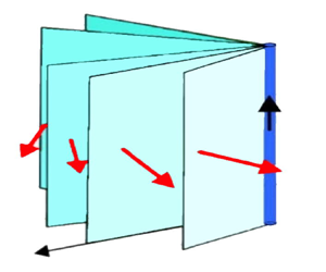
The situation changes when a vortex defect is present. Geometrically a nodal line  $\mathcal {L}$ is a simple, closed curve in $\mathbb {R}^3$, locus of intersection of a fan of isophase surfaces $\mathcal {S}$ hinged on $\mathcal {L}$, that foliate the entire fluid domain $\mathcal {D}$ (see figure 1). In this situation the vorticity $\boldsymbol {\omega }$ is localised on $\mathcal {L}$, and it can be described by a Dirac delta distribution. Since higher-order charge defects are known to be unstable and decay to a multiplet of unit charge vortex lines (Kuopanportti & Möttönen Reference Kuopanportti and Möttönen2010), we shall restrict our attention to defects of unit strength, taking the vortex circulation $\varGamma _{GPE}=2{\rm \pi}$. We have
 \begin{equation} \boldsymbol{\omega}(\boldsymbol{x}) =\oint_{\mathcal{L}} \delta^{(3)}(\boldsymbol{x}-\boldsymbol{s}(\sigma))\frac{\partial \boldsymbol{s}}{\partial \sigma}\, \mathrm{d}\sigma =\delta_{\mathcal{L}}({\boldsymbol{x}})\hat{\boldsymbol{t}}=\boldsymbol{\delta}_{\mathcal{L}}({\boldsymbol{x}}) , \end{equation}
where  $\delta ^{(3)}(\boldsymbol {x})$ is Dirac's delta function in $\mathbb {R}^3$, $\boldsymbol {s}=\boldsymbol {s}(\sigma )$ the instantaneous configuration of $\mathcal {L}$ (parametrized by $\sigma$) and $\hat {\boldsymbol {t}}$ the unit tangent to ${\mathcal {L}}$. The vortex circulation defined in terms of $\boldsymbol {\nabla } \theta$ will be quantized because (as we shall see below) the phase is multi-valued, regaining the original value after a whole number of turns around $\mathcal {L}$. Since vortices correspond to nodal lines where the density vanishes, the fluid domain is no longer simply-connected, and the phase becomes multi-valued. The phase single-valuedness is restored by the insertion of Riemann's cuts, which leads to a correction of the velocity field. By applying Kleinert's (Reference Kleinert2008) theory of currents (seen as Schwartz distributions on the space of differential forms), we can demonstrate (see Ricca & Foresti Reference Ricca, Foresti and Liu2022) that up to constants we have
 \begin{equation} \boldsymbol{u}(\boldsymbol{x}) = \boldsymbol{\nabla} \theta({\boldsymbol{x}})+ \boldsymbol{\delta}_\varSigma (\boldsymbol{x}) , \end{equation}
where  $\varSigma$ represents a (virtual) cut isophase surface, and $\boldsymbol {\delta }_\varSigma (\boldsymbol {x})=\int _\varSigma \delta ^{(3)}({\boldsymbol {x}}-{\boldsymbol {x}}')\,\hat {\boldsymbol {\nu }}\,\mathrm {d}^2{\boldsymbol {x}}'$ ( $\hat {\boldsymbol {\nu }}$ unit normal to $\varSigma$). Evidently the velocity does not depend on the choice of $\varSigma$, so that
 \begin{equation} \boldsymbol{\omega}(\boldsymbol{x})=\boldsymbol{\nabla} \times \boldsymbol{u}(\boldsymbol{x}) =\boldsymbol{\nabla} \times \boldsymbol{\delta}_\varSigma({\boldsymbol{x}})=\boldsymbol{\delta}_{\mathcal{L}} (\boldsymbol{x})\neq\boldsymbol{0} , \end{equation}
as expected.

Figure 1. Distinguished isophase surfaces (shades of cyan)  $\mathcal {S}_0$, $\mathcal {S}_1$, $\mathcal {S}_2$, $\ldots$ associated with (a) a straight vortex, and (b) a vortex ring. The induced velocity field ${\boldsymbol {u}}$ is represented by red arrows.
2. Helicity as a Noether charge in Euler fluids and superfluids
Consider the class of diffeomorphisms  $\boldsymbol {\varphi }_t\in \mathrm {Diff}(\mathcal {D})$ of the fluid domain $\mathcal {D}\subseteq \mathbb {R}^3$ such that $\boldsymbol {\varphi }_t: \mathcal {D}\to \mathcal {D}$, with time $t\in [0,T]\subset \mathbb {R}$. Under the action of the Lagrangian flow map $\boldsymbol {\varphi }$ fluid particles at the initial position ${\boldsymbol {a}}$ will be transported to the final position ${\boldsymbol {x}}$. For any smooth function, conservation of circulation and helicity (as a result of the topological invariance of the velocity field) can be proven by Noether's theorem by standard particle relabelling symmetry techniques (Bretherton Reference Bretherton1970; Lynden-Bell & Katz Reference Lynden-Bell and Katz1981; Salmon Reference Salmon1988; Yahalom Reference Yahalom1995; Fukumoto Reference Fukumoto2008). Here we show that the same derivation can be equally applied to the GPE case by using distributional techniques. To do this let us briefly recall this derivation for Euler's fluid first. The Euler action is given by
 \begin{equation} S_{E}=\int_T \mathrm{d} t \int_\mathcal{D} \rho\left(\frac{1}{2}|{\boldsymbol{u}}|^2-e(\rho)\right) \mathrm{d}^3{\boldsymbol{x}} =\int_T \mathrm{d} t \int_\mathcal{D} \ell_E({\boldsymbol{u}},\rho)\,\mathrm{d}^3{\boldsymbol{x}} , \end{equation}
where  ${\boldsymbol {u}}={\boldsymbol {u}}({\boldsymbol {x}},t)=D_t{\boldsymbol {x}}=\partial _t{\boldsymbol {x}}+({\boldsymbol {u}}\boldsymbol {\cdot } \boldsymbol{\nabla} ){\boldsymbol {x}}$ denotes the velocity field (with $D_t$ the Lagrangian derivative), $\rho =\rho ({\boldsymbol {x}},t)$ the fluid density, $e(\rho )$ the specific internal energy and $\ell _E=\ell _E({\boldsymbol {u}},\rho )$ the standard Lagrangian density for Euler's flow. The Noether charge is given by the variation of the action $S_{E}$ due to the particle relabelling $\tilde {a}_i=a_i+\varepsilon \eta _i$ ( $\varepsilon$ being the perturbation parameter and $\eta_i$ the displacement component). We have
 \begin{equation} \delta S_{E}=\int_T \mathrm{d} t \int_\mathcal{D} \left(\frac{\partial {\ell_E}}{\partial u_i}\delta u_i +\frac{\partial {\ell_E}}{\partial \rho}\delta \rho\right)\mathrm{d}^3{\boldsymbol{x}} , \end{equation}
since  $\delta x_i=0$ implies $(\partial \ell _E/\partial x_i)\delta x_i=0$. Let $\boldsymbol {J}_{ij}=\partial x_i/\partial a_j$ be the Jacobian of the transformation from the initial to the final position, with determinant $J=\textrm {det}(\boldsymbol {J})$. Evidently we have $\rho /\rho _0=\rho ({\boldsymbol {x}},t)/\rho ({\boldsymbol {a}}, 0)=J^{-1}$. Without loss of generality let us take $\rho _0=1$; following Fukumoto (Reference Fukumoto2008), from $D_t{\boldsymbol {a}}=\boldsymbol {0}$ we have
 \begin{equation} u_i={-}(\boldsymbol{J})_{ij}\frac{\partial a_j}{\partial t} , \end{equation}
so that under the variation  $\delta a_j=\varepsilon \eta _j$, we can write
 \begin{equation} \delta u_i={-}(\boldsymbol{J})_{ij} \frac{\mathrm{D}}{\mathrm{D} t} \left(\varepsilon \eta_j\right) ; \end{equation}
moreover, since  $\rho _0=1$, we also have
 \begin{equation} \delta \rho =\rho\frac{\partial}{\partial a_j}\left(\varepsilon \eta_j\right) , \end{equation}
with boundary conditions  $\eta =0$ at $t=0$ and $t=T$ for all ${\boldsymbol {x}}\in \mathcal {D}$, and normal condition $\boldsymbol {\eta }\boldsymbol {\cdot } \hat {\boldsymbol {\nu }}=0$ on $\partial \mathcal {D}$. Now, notice that $D_t\eta _j=0$ implies that variations in relabelling leaves the velocity field unchanged ( $\delta u_i=0$), while $\partial _{a_j}\eta _j=0$ implies that density is invariant ( $\delta \rho =0$). Hence, from $\delta S_{E}=0$ and mass conservation $\rho \,\mathrm {d}^3 {\boldsymbol {x}}=\mathrm {d}^3 {\boldsymbol {a}}$, using (2.4)–(2.5) together with the boundary conditions, we obtain
 \begin{equation} \frac{\mathrm{D}}{\mathrm{D} t}\left(u_i \frac{\partial x_i}{\partial a_j}\eta_j\right) -\frac{\partial}{\partial x_j}\left(\frac{\partial \ell}{\partial \rho} \eta_j\right)=0 , \end{equation}
which gives the conservation of the Noether charge
 \begin{equation} Q_{E}= \int_\mathcal{D} u_i \frac{\partial x_i}{\partial a_j}\eta_j\, \mathrm{d}^3 {\boldsymbol{a}} . \end{equation}
2.1. Circulation  $\varGamma$

By applying a transformation that transports particles along a loop  $\mathcal {C}$ defined by the vector position ${\boldsymbol {a}}(s)$ ( $s$ arclength), we have
 \begin{equation} \eta_j=\oint_{\mathcal{C}} \delta^{3}({\boldsymbol{a}}-{\boldsymbol{a}}(s))\frac{\partial a_j(s)}{\partial s}\, \mathrm{d} s ; \end{equation}
in this case the conservation of  $Q_E$ gives Kelvin's circulation theorem:
 \begin{equation} Q_{E}=\int_\mathcal{D} u_i \frac{\partial x_i}{\partial a_j}\eta_j\, \mathrm{d}^3 {\boldsymbol{a}} =\oint_\mathcal{C} {\boldsymbol{u}} \boldsymbol{\cdot} \left(\boldsymbol{J}\frac{\partial {\boldsymbol{a}}(s)}{\partial s}\right) \mathrm{d} s =\oint_\mathcal{C} \boldsymbol{u} \boldsymbol{\cdot}\frac{\partial {\boldsymbol{x}}(s)}{\partial s}\, \mathrm{d} s=\varGamma . \end{equation}
2.2. Helicity $H$

Consider the transformation that transports particles around a vortex line in  $\mathcal {D}$; from Fukumoto (Reference Fukumoto2008), we have
 \begin{equation} \eta_j=\epsilon_{jlk}\frac{\partial u^h}{\partial a_l}\frac{\partial x_h}{\partial a_k} , \end{equation}
where  $\epsilon _{jlk}$ is the Levi–Civita tensor. By Euler's equations, and the anti-symmetry property of the tensor $\epsilon$, we can verify that the transformation (2.10) satisfies the relabelling symmetry condition. Moreover, by using the identity $\epsilon _{jlk}\det (\boldsymbol {A})=\epsilon _{irh}a^{ij}a^{rl}a^{hk}$ and (2.10), the $Q_E$ density becomes
 \begin{equation} u_i\frac{\partial x_i}{\partial a_j}\eta_j =u_i\frac{\partial x_i}{\partial a_j}\epsilon_{jlk}\frac{\partial u^h}{\partial a_l}\frac{\partial x_h}{\partial a_k} =u_i J \epsilon_{irh}\frac{\partial u^h}{\partial a_l}\frac{\partial a_l}{\partial x_r} =u_i J ( \boldsymbol{\nabla} \times \boldsymbol{u})_i =u_i J\omega_i \end{equation}
so that
 \begin{equation} Q_E=\int_\mathcal{D} u_i\frac{\partial x_i}{\partial a_j}\eta_j\,\mathrm{d}^3{\boldsymbol{a}} =\int_\mathcal{D} u_i \omega_i J\,\mathrm{d}^3{\boldsymbol{a}} =\int_\mathcal{D} \boldsymbol{u} \boldsymbol{\cdot} \boldsymbol{\omega}\,\mathrm{d}^3{\boldsymbol{x}}=H . \end{equation}
2.3. The GPE case
Now let us consider the action of the GPE; from the non-dimensional form of (1.2), and by using (1.4) and (1.8), the action associated with (1.3) can be written as
 \begin{equation} S_{GPE}={-}\int_T {\rm d}t\int_{\mathcal{D}} \rho\left(\frac{\partial\theta}{\partial t} + \frac12(\boldsymbol{\nabla} \theta+\boldsymbol{\delta}_\varSigma)^2-h(\rho)\right) \mathrm{d}^3{\boldsymbol{x}} , \end{equation}
where  $h(\rho )$ (that plays the role of a quantum internal energy) is a given function of the density $\rho$ and its gradients. We can prove the following result.
Theorem 2.1 A system governed by the GPE given by (1.3) has circulation  $\varGamma _{GPE}$ and helicity $H_{GPE}$ given by
 \begin{equation} \quad\varGamma_{GPE}=\oint_\mathcal{C}{\boldsymbol{u}}\boldsymbol{\cdot}\mathrm{d}\kern0.7pt {\boldsymbol{x}}=2{\rm \pi} n , \quad \quad H_{GPE}=\int_\mathcal{D}{\boldsymbol{u}}\boldsymbol{\cdot}\boldsymbol{\omega}\,\mathrm{d}^3{\boldsymbol{x}}=0 . \end{equation}
Proof. In order to establish the relation between  $S_{GPE}$ and $S_E$, let us first re-write
 \begin{equation} \frac{\partial\theta}{\partial t}=\frac{\mathrm{D}\theta}{\mathrm{D} t}-({\boldsymbol{u}}\boldsymbol{\cdot}\boldsymbol{\nabla})\theta =\frac{\mathrm{D}\theta}{\mathrm{D} t}-[(\boldsymbol{\nabla} \theta+\boldsymbol{\delta}_\varSigma)\boldsymbol{\cdot}\boldsymbol{\nabla}]\theta =\frac{\mathrm{D}\theta}{\mathrm{D} t}-|\boldsymbol{\nabla} \theta|^2-\boldsymbol{\delta}_\varSigma\boldsymbol{\cdot}\boldsymbol{\nabla} \theta . \end{equation}
From (1.8), we have that  $|{\boldsymbol {u}}|^2=|\boldsymbol {\nabla } \theta |^2+2\boldsymbol {\delta }_\varSigma \boldsymbol {\cdot }\boldsymbol {\nabla } \theta +| \boldsymbol {\delta }_\varSigma |^2$; (2.15) can thus be re-written as $\partial _t\theta =D_t\theta -|{\boldsymbol {u}}|^2+\boldsymbol {\delta }_\varSigma \boldsymbol {\cdot }\boldsymbol {\nabla } \theta +|\boldsymbol {\delta }_\varSigma |^2$. Substituting this last expression into (2.13), we have
 \begin{equation} S_{GPE}={-}\int_T {\rm d}t\int_\mathcal{D} \rho\left(\frac{\mathrm{D}\theta}{\mathrm{D} t} - \frac12|{\boldsymbol{u}}|^2+\boldsymbol{\delta}_\varSigma\boldsymbol{\cdot}\boldsymbol{\nabla} \theta+|\boldsymbol{\delta}_\varSigma|^2 -h(\rho)\right) \mathrm{d}^3{\boldsymbol{x}} . \end{equation}
By using the divergence theorem, the third contribution above becomes
 \begin{equation} \int_\mathcal{D}\boldsymbol{\delta}_\varSigma\boldsymbol{\cdot}\boldsymbol{\nabla} \theta\,\mathrm{d}^3{\boldsymbol{x}} =\int_\mathcal{D} \boldsymbol{\nabla} \boldsymbol{\cdot} (\boldsymbol{\delta}_\varSigma\theta)\,\mathrm{d}^3{\boldsymbol{x}} =\int_{\varSigma}\theta(\boldsymbol{\delta}_\varSigma \boldsymbol{\cdot}\boldsymbol{\hat\nu})\,\mathrm{d}^2{\boldsymbol{x}} =\theta_{\varSigma}\int_{\varSigma}\boldsymbol{\delta}_\varSigma \boldsymbol{\cdot}\boldsymbol{\hat\nu}\,\mathrm{d}^2{\boldsymbol{x}} , \end{equation}
where  $\theta _{\varSigma }$ is the value of $\theta$ restricted to $\varSigma$, and it is constant and independent of time. Moreover $|\boldsymbol {\delta }_\varSigma |$ is also constant and independent of time: from Kleinert (Reference Kleinert2008, p. 201, (6.33)), we have
 \begin{equation}
\frac{\mathrm{d}}{\mathrm{d}
t}|\boldsymbol{\delta}_\varSigma|^2
=2[\boldsymbol{\delta}_\varSigma\boldsymbol{\cdot}\left({\boldsymbol{u}}\times(\boldsymbol{\nabla}
\times\boldsymbol{\delta}_\varSigma)\right)]
=[(\boldsymbol{\nabla}
\times\boldsymbol{\delta}_\varSigma)\boldsymbol{\cdot}(\boldsymbol{\delta}_\varSigma\times{\boldsymbol{u}})],
\end{equation}
\begin{equation}
\frac{\mathrm{d}}{\mathrm{d}
t}|\boldsymbol{\delta}_\varSigma|^2
=2[\boldsymbol{\delta}_\varSigma\boldsymbol{\cdot}\left({\boldsymbol{u}}\times(\boldsymbol{\nabla}
\times\boldsymbol{\delta}_\varSigma)\right)]
=[(\boldsymbol{\nabla}
\times\boldsymbol{\delta}_\varSigma)\boldsymbol{\cdot}(\boldsymbol{\delta}_\varSigma\times{\boldsymbol{u}})],
\end{equation}
but
 \begin{equation} \int_\mathcal{D}(\boldsymbol{\delta}_\varSigma\times{\boldsymbol{u}})\,\mathrm{d}^3{\boldsymbol{x}} =\int_{\varSigma}(\boldsymbol{\hat\nu}\times{\boldsymbol{u}})\,\mathrm{d}^2{\boldsymbol{x}}=\boldsymbol{0} , \end{equation}
because  $\boldsymbol {\hat \nu }$ and ${\boldsymbol {u}}$ are everywhere pointwise parallel on $\varSigma$; hence $\mathrm {d} |\boldsymbol {\delta }_\varSigma |^2/\mathrm {d} t=0$. By absorbing these two constants into $h(\rho )$, we have
 \begin{equation} S_{GPE}=\int_T {\rm d}t \int_\mathcal{D} \rho\left(\frac12|{\boldsymbol{u}}|^2 - h(\rho)-\frac{\mathrm{D}\theta}{\mathrm{D} t}\right) \mathrm{d}^3{\boldsymbol{x}} =\int_T {\rm d}t \int_\mathcal{D} \ell_{GPE}({\boldsymbol{u}},\rho,\theta)\, \mathrm{d}^3{\boldsymbol{x}} ; \end{equation}
we can regard  $\ell _{GPE}$ as the sum of the densities $\ell _E$ and $\ell _\theta$ associated with an Euler action and a phase contribution, so that
 \begin{equation} S_{GPE}=\int_T \mathrm{d} t \int_\mathcal{D} \left[\ell_E({\boldsymbol{u}},\rho)+\ell_\theta(\theta)\right]\mathrm{d}^3{\boldsymbol{x}} =S_{E}+S_{\theta} . \end{equation}
Now, let's apply Noether's theorem following the same procedure as for the Euler context. Considering the variation of  $S_{GPE}$, and using the results above, we have the conservation of the GPE charge $Q_{GPE}$, where
 \begin{equation}
Q_{GPE}=Q_{E}+Q_{\theta} =\int_\mathcal{D}
u_i\frac{\partial x_i}{\partial a_j}\eta_j\,
\mathrm{d}^3{\boldsymbol{a}}-\int_\mathcal{D}
\frac{\partial \theta}{\partial a_j}\eta_j\,
\mathrm{d}^3{\boldsymbol{a}} .
\end{equation}
\begin{equation}
Q_{GPE}=Q_{E}+Q_{\theta} =\int_\mathcal{D}
u_i\frac{\partial x_i}{\partial a_j}\eta_j\,
\mathrm{d}^3{\boldsymbol{a}}-\int_\mathcal{D}
\frac{\partial \theta}{\partial a_j}\eta_j\,
\mathrm{d}^3{\boldsymbol{a}} .
\end{equation}In the presence of a defect, the velocity must take into account the multi-valuedness of the phase; by direct substitution of (1.8) into (2.22), we have
 \begin{equation} Q_{GPE}=\int_\mathcal{D} [\boldsymbol{\delta}_{\varSigma}({\boldsymbol{x}})]_i\frac{\partial x_i}{\partial a_j}\eta_j\, \mathrm{d}^3{\boldsymbol{a}}\neq0 . \end{equation}
By considering a loop  $\mathcal {C}\subset \mathbb {R}^3$ encircling a defect, and using (2.8), we have the conservation of the GPE circulation, i.e.
 \begin{equation} Q_{GPE}=\int_\mathcal{D} [\boldsymbol{\delta}_{\varSigma}({\boldsymbol{x}})]_i\frac{\partial x_i}{\partial a_j}\eta_j\, \mathrm{d}^3{\boldsymbol{a}} =\oint_\mathcal{C} \boldsymbol{\delta}_{\varSigma}({\boldsymbol{x}}) \boldsymbol{\cdot} \frac{\partial{\boldsymbol{x}}(s)}{\partial s}\,\mathrm{d} s=\varGamma_{GPE}=2{\rm \pi} n , \end{equation}
which proves (2.14a). Here  $n\in \mathbb {N}$ is associated with the multi-valuedness of $\theta$, and it represents the topological charge of the defect; $n$ is the winding number, and it is given by the number of intersections of the loop $\mathcal {C}$ with an isophase surface $\mathcal {S}$ spanning the nodal line $\mathcal {L}$.
Furthermore, by using (2.11) we also have
 \begin{equation} Q_{GPE}=\int_\mathcal{D} [\boldsymbol{\delta}_{\varSigma}({\boldsymbol{x}})]_i\frac{\partial x_i}{\partial a_j}\eta_j\, \mathrm{d}^3{\boldsymbol{a}} =\int_\mathcal{D} \boldsymbol{\delta}_{\varSigma}({\boldsymbol{x}}) \boldsymbol{\cdot} \boldsymbol{\omega} \, \mathrm{d}^3{\boldsymbol{x}} . \end{equation}
In the presence of a defect, the condensate ambient space is entirely foliated by infinitely many, smooth, isophase surfaces, all bounded by, and hinged upon the same defect. Let  $\mathcal {S}_1$ and $\mathcal {S}_2$ be two of such surfaces (see, for instance, figure 1b), and $\bar {\mathcal {S}}:=\mathcal {S}_1 \cup \mathcal {S}_2$ the union of $\mathcal {S}_1$ and $\mathcal {S}_2$; since $\bar {\mathcal {S}}$ is a closed surface in $\mathbb {R}^3$, let $\varOmega$ be the volume enclosed by $\bar {\mathcal {S}}$, so that $\partial \varOmega =\bar {\mathcal {S}}$. Remembering that $\boldsymbol {\nabla } \theta ({\boldsymbol {x}})+ \boldsymbol {\delta }_\varSigma (\boldsymbol {x})$ does not depend on any specific isophase surface, we evidently have
 \begin{equation} \boldsymbol{\delta}_{\varSigma}({\boldsymbol{x}}) =\tfrac{1}{2} \left[\boldsymbol{\delta}_{\mathcal{S}_1}({\boldsymbol{x}})+\boldsymbol{\delta}_{\mathcal{S}_2}({\boldsymbol{x}})\right] . \end{equation}
Hence, by applying the divergence theorem to (2.25), we have
 \begin{equation} Q_{GPE}=\int_\mathcal{D} \boldsymbol{\delta}_{\varSigma}({\boldsymbol{x}}) \boldsymbol{\cdot} \boldsymbol{\omega} \, \mathrm{d}^3{\boldsymbol{x}} =\int_{\bar{\mathcal{S}}} \boldsymbol{\omega} \boldsymbol{\cdot} \hat{\boldsymbol{\nu}}\, \mathrm{d}^2{\boldsymbol{x}} =\int_{\varOmega} \boldsymbol{\nabla} \boldsymbol{\cdot} \boldsymbol{\omega}\, \mathrm{d}^3{\boldsymbol{x}}=0 , \end{equation}
since  $\boldsymbol {\delta }_{\varSigma }({\boldsymbol {x}})$ is normal to any isophase surface, and $\boldsymbol {\omega }$ is a solenoidal field. Since the irrotational part of the velocity does not contribute to the kinetic helicity, by using (1.8) and (2.27), we have
 \begin{equation} Q_{GPE}=\int_\mathcal{D} \boldsymbol{\delta}_{\varSigma}({\boldsymbol{x}}) \boldsymbol{\cdot} \boldsymbol{\omega} \, \mathrm{d}^3{\boldsymbol{x}}= \int_\mathcal{D} \boldsymbol{u} \boldsymbol{\cdot} \boldsymbol{\omega}\,\mathrm{d}^3{\boldsymbol{x}}=H_{GPE}=0 , \end{equation}
which proves (2.14b).
We should emphasize that the result above can only be proven by using distributional techniques; indeed, by relying on smooth functions Kedia et al. (Reference Kedia, Kleckner, Scheeler and Irvine2018) simply show that the helicity is zero because the Noether charge is always zero under any transformation, a result that cannot hold true for circulation (which is generally non-zero), and hence that cannot be taken as a proof for the conservation of the vanishing helicity.
The results of Theorem 2.1 are independent from the number of defects present in the system, and their geometric and topological configuration. The particular case of a vortex ring threaded by a co-axial, straight defect where an additional localised vorticity field is present on the central nodal line, for instance, has been investigated by numerical simulations (Zuccher & Ricca Reference Zuccher and Ricca2018), and studied extensively by Foresti & Ricca (Reference Foresti and Ricca2019, Reference Foresti and Ricca2020, Reference Foresti and Ricca2022a,Reference Foresti and Riccab). As demonstrated there, the existence of a localised field on the intersection of the isophase foliation is just the natural consequence of the emergence of a new topological phase, in agreement with the simultaneous presence of distributional currents (Onural Reference Onural2006), and the zero helicity condition.
3. The zero helicity condition from a topological viewpoint
As shown by Salman (Reference Salman2017), the topological decomposition of the kinetic helicity of quantum defects in terms of linking numbers, derived by Moffatt (Reference Moffatt1969) and Moffatt & Ricca (Reference Moffatt and Ricca1992), holds true also for the GPE case. Since any isophase of a defect is an orientable surface bounded by the defect (i.e. it is a Seifert surface), we can use this surface to compute linking numbers, and show (Salman Reference Salman2017) that for a suitably defined frame of reference (i.e. a Seifert framing) total helicity (that is independent of the reference frame) is always zero. For a system of  $N$ defects of unit strength ( $\varGamma _{GPE}=2{\rm \pi}$), one can prove (Sumners et al. Reference Sumners, Cruz-White and Ricca2021) that
 \begin{equation} H_{GPE}=\sum_i Sl_i+\sum_{i\neq j}Lk_{ij}=0 \quad(i,j=1,\ldots,N) , \end{equation}
where  $Sl_i$ and $Lk_{ij}$ are respectively the self-linking and the linking number of the defects. This means that a system of defects can only exist if the topological requirement of zero total linking is satisfied; a network of defects can thus form only if the amount of mutual linking is balanced by the total writhe and twist of the individual vortex lines. For instance, as discussed in relation to the example mentioned in the previous section, the superposition of a twist phase on a single defect in isolation induces the creation of a new, secondary defect that threads the former to keep the total linking number zero (Foresti & Ricca Reference Foresti and Ricca2022b).
Since  $Lk_{ij}=Lk_{ji}$, the linking coefficients can be arranged in a matrix form, given by
 \begin{equation} \boldsymbol{M}= \begin{bmatrix} Sl_{1} & Lk_{12} & \dots & Lk_{1N} \\ Lk_{12} & Sl_{2} & \dots & Lk_{2N} \\ \dots & \dots & \dots & \dots \\ Lk_{1N} & Lk_{2N} & \dots & Sl_{N} \end{bmatrix} , \end{equation}
where  $\boldsymbol {M}$ is real symmetric; for a given entry $i\in [1,N]$, (3.1) prescribes that the corresponding row/column elements of $\boldsymbol {M}$ must sum up to zero, a condition very little explored in matrix theory. Moreover, since any real symmetric matrix can be reduced to a diagonal form $\boldsymbol {D}$, assuming that the inverse $\boldsymbol {D}^{-1}$ exists, we can discover the self-linking conditions for $N$ co-existing, unlinked defects. This applies also for the existence of a single knot (say a trefoil) in isolation, for which writhe and total twist must always balance to zero in order to satisfy the requirement $Sl=0$. This information is useful to understand the long-term behaviour of a system of defects, because defects with twist different from zero are in general highly unstable, developing reconnections, and undergoing a rapid energy decay, with production of small vortex rings. Hence, taking advantage of the topological constraint (3.1) proves not only useful to create complex structural networks of defects, but it may well provide useful information for experimental and technological applications.
Funding
R.L.R. wishes to acknowledge financial support from the National Natural Science Foundation of China (grant no. 11572005).
Declaration of interests
The authors report no conflict of interest.
Author contributions
R.L.R. proposed and supervised the project, and wrote the paper; A.B. implemented the theory and performed the calculations.


 Open access