


1. Introduction
The study of drop impact physics began with the seminal works of Worthington in the late nineteenth century (Worthington Reference Worthington1877; Worthington & Cole Reference Worthington and Cole1897) and continues today due to applications in various industries like manufacturing, printing, food-processing, bio-medical and pharmaceuticals (Pasandideh-Fard, Chandra & Mostaghimi Reference Pasandideh-Fard, Chandra and Mostaghimi2002; Bolleddula, Berchielli & Aliseda Reference Bolleddula, Berchielli and Aliseda2010; Roy et al. Reference Roy, Pandey, Banik, Mukherjee and Basu2019). The early pioneering work of Worthington led to the discovery of various spatio-temporal physics during drop impacts on solids and liquids. Drop impacts on liquids generate aesthetically beautiful patterns like crowns, corona splashes and jets, to name a few (Gekle & Gordillo Reference Gekle and Gordillo2010; Gordillo & Gekle Reference Gordillo and Gekle2010) and are used in various artistic contexts and platforms. The mechanism underlying the beauty is multi-scale and multi-physics in origin and has attracted many scientists and engineers to study drop impacts on liquids theoretically, numerically and experimentally (Tropea & Marengo Reference Tropea and Marengo1999; Sikalo et al. Reference Sikalo, Marengo, Tropea and Ganic2000; Rioboo, Tropea & Marengo Reference Rioboo, Tropea and Marengo2001; Roisman & Tropea Reference Roisman and Tropea2002; Renardy et al. Reference Renardy, Popinet, Duchemin, Renardy, Zaleski, Josserand, Drumright-Clarke, Richard, Clanet and Quéré2003; Thoraval et al. Reference Thoraval, Takehara, Etoh, Popinet, Ray, Josserand, Zaleski and Thoroddsen2012). With the advent of ultra-high-speed imaging and laser diagnostic techniques (Lauterborn & Vogel Reference Lauterborn and Vogel1984; Adrian Reference Adrian1991; Thoroddsen, Etoh & Takehara Reference Thoroddsen, Etoh and Takehara2008; Versluis Reference Versluis2013) the spatio-temporal experimental resolution has increased by orders of magnitude from the early days of drop impact research (Worthington Reference Worthington1877; Worthington & Cole Reference Worthington and Cole1897).
A droplet impacting on a liquid medium can result in a wide variety of phenomena like splashing, bouncing, coalescence and formation of jets, corollas and crowns depending on the impact parameter space characterized by various non-dimensional groups like the impact Weber number, Reynolds number, Ohnesorge number, Bond number and Froude number to name a few (Thoroddsen et al. Reference Thoroddsen, Thoraval, Takehara and Etoh2011; Yarin, Roisman & Tropea Reference Yarin, Roisman and Tropea2017). The various non-dimensional numbers represent the ratios of various competing effects governing the dynamics of drop impacts. Several phenomena like the formation of a flower-like pattern in the liquid film, entrapment of air, generation and propagation of an ejectum sheet widen the landscape of possibilities of drop impact physics on liquids (Thoroddsen Reference Thoroddsen2002; Zhang et al. Reference Zhang, Toole, Fezzaa and Deegan2012; Marcotte et al. Reference Marcotte, Michon, Séon and Josserand2019). During the impinging process, just prior to impact, a thin lubricating air layer gets entrapped underneath the droplet (Thoroddsen, Etoh & Takehara Reference Thoroddsen, Etoh and Takehara2003; Bartolo, Josserand & Bonn Reference Bartolo, Josserand and Bonn2006). The entrapped air between the drop and the liquid must be displaced/drained out before proper contact between the drop and the pool. The pressure in the lubricating air layer is inversely proportional to the air layer thickness and hence increases monotonically till the entrapped air pressure reaches the capillary pressure of the droplet (Thoroddsen et al. Reference Thoroddsen, Etoh and Takehara2003; Hicks & Purvis Reference Hicks and Purvis2010, Reference Hicks and Purvis2011; Roy et al. Reference Roy, Sophia, Rao and Basu2022). The excess pressure above the capillary pressure causes a dimple to form just beneath the impacting droplet. The air layer ruptures at a point leading to the first local contact of the drop and the formation of entrapped air bubbles. The formation of air bubbles in drop impact systems can be detrimental to specific technologies such as printing, coating and several cooling applications (Aziz & Chandra Reference Aziz and Chandra2000; Yarin et al. Reference Yarin, Roisman and Tropea2017; Aksoy et al. Reference Aksoy, Zhu, Eneren, Koos and Vetrano2020). However, the entrapment of air bubbles is a boon to aquatic life forms since these entrapped air bubbles are a medium of gaseous exchange between the atmosphere and the water bodies that sustain marine life forms (Woolf et al. Reference Woolf2007). For impacts on similar liquids, after the initial entrapped air layer rupture phase, the droplet forms an air crater in the liquid layer/pool, collapsing to form Worthington jets. The singularity dynamics and curvature collapse leading to jet eruption on a fluid surface were studied in a seminal work by Zeff et al. (Reference Zeff, Kleber, Fineberg and Lathrop2000). Further, in the previous decade, Gekle and Gordillo studied the Worthington jet formed during the impact of a circular disc on water using detailed boundary-integral simulations and analytical modelling (Gekle & Gordillo Reference Gekle and Gordillo2010; Gordillo & Gekle Reference Gordillo and Gekle2010). They discovered that the flow structure inside the jet could be divided into three regions; the acceleration region, ballistic region and tip region. A majority of the previous studies on drop impact on liquids have focused on impacts on similar liquids (Shetabivash, Ommi & Heidarinejad Reference Shetabivash, Ommi and Heidarinejad2014; Castillo-Orozco et al. Reference Castillo-Orozco, Davanlou, Choudhury and Kumar2015; Castrejón-Pita et al. Reference Castrejón-Pita, Muñoz-Sánchez, Hutchings and Castrejón-Pita2016; Yarin et al. Reference Yarin, Roisman and Tropea2017; Hasegawa & Nara Reference Hasegawa and Nara2019). However, the literature of drop impacts on immiscible pools is relatively sparse (Yakhshi-Tafti, Cho & Kumar Reference Yakhshi-Tafti, Cho and Kumar2010; Dhuper, Guleria & Kumar Reference Dhuper, Guleria and Kumar2021; Che & Matar Reference Che and Matar2018; Minami & Hasegawa Reference Minami and Hasegawa2022). Drop impacts on immiscible liquid pools are very important and is found in various industrial, engineering and natural systems. Droplet interactions in immiscible systems are inherently different, as mentioned in some of the literature available (Che & Matar Reference Che and Matar2018). In general, drop impact on liquids produces Worthington jets (Worthington & Cole Reference Worthington and Cole1897) on the liquid pool formed due to the collapse of an air crater in the liquid pool. However, we have found that the air craters formed in immiscible impact systems are significantly different from those reported in the literature for miscible liquids. Primarily, the air crater on the surface of the impacting droplet resembles central air craters found in drop impacts on superhydrophobic substrates (Yamamoto, Motosuke & Ogata Reference Yamamoto, Motosuke and Ogata2018) at low impact Weber number. Locally, the air craters on the drop surface can be understood based on the response dynamics of the droplet subjected to external forces, as was demonstrated by Harper, Grube & Chang (Reference Harper, Grube and Chang1972) and Simpkins & Bales (Reference Simpkins and Bales1972). The similarity between air craters/jets observed on droplet surfaces during impact on viscous immiscible liquid pools to jets/craters observed on droplets surface impacting a hydrophobic surface led us to map the immiscible liquid impact problem to the constrained Rayleigh drop eigenvalue problem (Strani & Sabetta Reference Strani and Sabetta1984; Bostwick & Steen Reference Bostwick and Steen2009, Reference Bostwick and Steen2013a,Reference Bostwick and Steenb, Reference Bostwick and Steen2014, Reference Bostwick and Steen2015), as was done by Kern et al. for drop impacts on solid surfaces (Kern, Bostwick & Steen Reference Kern, Bostwick and Steen2021). Recent studies have shown various topologies of air crater/singular jet formation in immiscible impacts (Yang, Tian & Thoroddsen Reference Yang, Tian and Thoroddsen2020). However, the detailed mechanism of the jets produced on the surface of the droplets is not well understood and remains elusive.
A general three-fluid immiscible system dealing with impact scenarios labelled as  $1,2,3$ is described by the following physical parameters: the densities $({\rho }_1,{\rho }_2,{\rho }_3)$; the viscosities $({\mu }_1,{\mu }_2,{\mu }_3)$; the pairwise surface tensions $({\sigma }_{12},{\sigma }_{13},{\sigma }_{23})$; the impact velocity $V_0$; acceleration due to gravity $g$; and the radius of the droplet $R_0$. Overall, there are $12$ dimensional parameters to fully characterize the general dynamics of the impacting system. Using the Buckingham Pi theorem (Barenblatt Reference Barenblatt1996) we can construct $9$ non-dimensional parameters to reduce the parameter space. The non-dimensional parameters are ${\rho }_1/{\rho }_2$, ${\rho }_2/{\rho }_3$, ${\mu }_1/{\mu }_2$, ${\mu }_2/{\mu }_3$, ${\sigma }_{12}/{\sigma }_{13}$, ${\sigma }_{13}/{\sigma }_{23}$, $We$,
$We$,  $Ca$,
$Ca$,  $Fr$, where $We$,
$We$,  $Ca$ and $Fr$ are the Weber, capillary and Froude numbers, respectively. We observe that, of the $9$ non-dimensional quantities, only $3$ quantities are related to the dynamics and the remaining $6$ quantities specify the fluid properties and define the particular fluids used. For a given set of fluids, the dynamics could be characterized based on the triplets ( $We, Ca, Fr$). The Weber number based on the droplet diameter is defined as $We={\rho }_wV_0^22R_0/{\sigma }_{aw}$, where ${\rho }_w$ is the density of the impacting droplet, $V_0$ is the impact velocity and ${\sigma }_{aw}$ is the air–water surface tension. The capillary number is defined as $Ca={\mu }_sV_0/{\sigma }_{aw}$, where ${\mu }_s$ is the viscosity of the silicone-oil pool. The Froude number is defined as $Fr=V_0/{gR_0}$. Note that the three triplets $(We,Ca,Fr)$ are monotonically increasing functions of the impact velocity $V_0$. The Weber number depends on the impact velocity quadratically whereas the capillary and Froude number vary linearly.
The main experimental control parameter used in this work is the impact velocity and hence the Weber number has the largest variation in terms of numerical values. We use the Weber number to characterize all the observations experimentally since an order of magnitude change is observed in  $We$ due to the variation in the range of $V_0$. Note, however, for different values of Weber number, the capillary number and the Froude number are uniquely defined and any impact event in the current experimental context of the work requires a triplet of $(We, Ca, Fr)$ to uniquely define an impact event. In general, the force involved to cause droplet retardation is viscous drag. However, the observed response of the droplet is governed by inertia and surface tension. This is due to the fact that the impacting droplet is approximately $350$ times less viscous than the silicone-oil pool. The experimental response time scale of the droplet is within the capillary time scale ( $t_c\sim {O}(9\times 10^{-3}\ {\rm s})$). The viscous effects inside the droplet are important at the scale of the viscous diffusion time scale ( ${\sim }{O}(4R_0^2/{\nu }_w)=5.43\ {\rm s}$). We should realize that the droplet response occurs at a scale of milliseconds, which is three orders of magnitude smaller than the viscous diffusion time scale inside the droplet. Therefore, we can use Weber number to describe the crater observations in general. Further, the high viscosity of the pool ensures that the surface of the droplet below the dynamic contact line has negligible modal oscillations due to high dissipation. The time scale of the viscous dissipation in the liquid pool is of the order of the air crater response time scale ( ${\sim }{O}(4R_0^2/{\nu }_s)\sim 10\times 10^{-3}\ {\rm s}\sim t_c$). In this work, we study the role of impact Weber number ( $We={\rho }_wV_0^22R_0/{\sigma }_{aw}$) on the formation of air craters on the surface of an impacting water droplet on an immiscible highly viscous liquid pool of silicone oil with particular focus on the mechanism of air crater formation using experimental and theoretical analyses.
The remaining text is organized as follows. In § 2, we provide the details of the experimental set-up and data processing methods. Section 3 outlines the results and discussions with various subsections. Section 3.1 provides a global overview of the important results obtained. Section 3.2 discusses droplet penetration dynamics and the scales of the various forces acting on the droplet. Section 3.3 details ways of characterizing droplet deformation from the spherical shape. Section 3.4 provides a criterion for forming air craters of significant depth. Section 3.5 computes the centre of mass velocity of the droplet. Section 3.6 outlines the details of droplet response/air crater and jet characteristics from a local analysis viewpoint. Section 3.7 discusses the droplet response from a constrained Rayleigh drop model perspective using the Green's function method to solve an eigenvalue problem. We conclude with the results and future scope in § 4.
The underlying theme of the current work was to identify the mechanisms and mechanics involved in the droplet surface crater formation of the air–water interface of the impacting droplet on an immiscible high viscous liquid pool. The detailed characterization for various experimental parameter ranges is outside the scope of the present work.
2. Materials and methods
Figure 1(a) shows a schematic representation of the experimental set-up for the high-speed imaging. The various components labelled in the schematic representation are a syringe pump (New Era Pump Systems, NE-1010); syringe and a hypodermic needle; stroboscopic light source; a diffuser plate; water droplet; acrylic container; silicone-oil pool; computer with image acquisition software and high-speed cameras (Photron Fastcam Mini UX100, Photron Fastcam SA5) with Tokina and Navitar zoom lens. The small red dotted rectangle represents the region of interest for all experimental imaging. The dotted straight line  $1-0$ and $2-0$ represents the visual axis of the high-speed camera for image acquisition. De-ionized water droplet of radius ( $R_0=1.1\pm 0.1\ {\rm mm}$) was used as the impacting liquid droplet. Silicone oil was used as the liquid pool, and the pool depth was maintained constant at $H_p\sim 5\ {\rm mm}$. The kinematic viscosity of the pool used was ${\nu }_{s}=350\ {\rm cSt}$ and density was ${\rho }_s\sim 970\ {\rm kg}\ {\rm m}^{-3}$. All experiments were conducted at room temperature of $T\sim 298\ {\rm K}$. The droplet impacts energy was varied by changing the impact velocity ( $0.3\unicode{x2013}2.2\ {\rm m}\ {\rm s}^{-1}$), and hence the triplet of non-dimensional numbers, impact Weber number, capillary number and Froude number ( $We, Ca, Fr$), was varied by changing the free fall height of the droplet from the free surface of the liquid pool using a vertical linear stage. We explored the formation mechanism of air crater on the surface of the droplet in regime $(We,Ca,Fr)=(4\unicode{x2013}145,1.7\unicode{x2013}10.27,3.48\unicode{x2013}20.97)$. The high-speed imaging was performed at 10 kHz ( $10^4$ frames per second) with a spatial resolution of $1.5$ micrometres per pixel (equivalent pixel density of
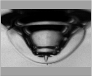
  ${\sim }666.667\ {\rm pixels}\ {\rm mm}^{-1}$). Figure 1(b) shows a high-speed time sequence images depicting the formation of surface craters on the impacting droplet at impact Weber number $We=65$. The timestamps are in milliseconds and the scale bar represents 1.56 mm. The acquired high-speed images were processed through an image processing pipeline consisting of background subtraction, image segmentation through an adaptive thresholding operation, followed by binarization and edge detection. The geometrical and kinematic quantities like droplet size and velocity were computed through various imaging processing shape descriptors using the image processing software ImageJ (Schneider, Rasband & Eliceiri Reference Schneider, Rasband and Eliceiri2012) and various in-house image processing codes written in Python (Van Rossum & Drake Reference Van Rossum and Drake2009) utilizing image processing libraries like opencv (Bradski Reference Bradski2000; Bradski & Kaehler Reference Bradski and Kaehler2008) and scikit-image (Van der Walt et al. Reference Van der Walt, Schönberger, Nunez-Iglesias, Boulogne, Warner, Yager, Gouillart and Yu2014). The geometrical parameters extracted from the images that were taken from an oblique visual axis of the camera (figure 1a) were corrected using appropriate trigonometric and affine transformations (Che & Matar Reference Che and Matar2018; Chityala & Pudipeddi Reference Chityala and Pudipeddi2020).

Figure 1. (a) Schematic of the experimental set-up used for high-speed imaging (not to scale). The various components of the set-up are labelled in the figure. The red dotted rectangle represents the region of interest. The dashed straight line  $1-0$ and $2-0$ represents the visual axis (different sightline) of the camera used during high-speed imaging experiments. (b) Time sequence images for impact Weber number $We=65$ depicting the formation of air craters. Scale bar represents 1.56 mm and timestamps are in milliseconds. (c) Schematic representing the air–water interface deformation process as a function of time leading to the formation of air craters. The arrows depict the direction of air–water interface propagation. The white line depicts the dynamic contact line that travels towards the north pole relative to the impacting droplet.
3. Results and discussions
3.1. Global overview
We discover that the mechanism behind air crater formation is (figure 1c) intricately related to the penetration dynamics of the impinging droplet through the liquid pool and depends on the impact Weber number. Figure 1(c) depicts the schematic representation of the surface crater formation on the air–water interface of the impacting droplet. Figure 2 shows the high-speed snapshots of a water droplet impacting a silicone liquid pool at various impact Weber numbers ( $We=4,16,65,145$). The timestamps are in milliseconds, and the scale bars represent 1 mm. The interaction between the silicone pool and water droplet occurs through the interplay of viscous, buoyancy, droplet weight, air–water and water–oil surface tension forces. Beyond a critical impact Weber number ( $We_c\sim 10$), air craters of significant depths (crater depth comparable to droplet size) are formed. No significant air craters are observed during the penetration phase for impact Weber number smaller than the critical Weber number ( $We< We_c$). The penetration time scale is largely increased due to the lubrication effect of the entrapped air layer formed under the droplet. The air layer rupture occurs at a time scale of the order of $t_r\sim 2\times 10^{-1}\ {\rm s}$. The transient dynamics of the droplet (surface oscillation) occurs early above the pool for $t< t_r$. For $t>t_r$, the droplet penetrates smoothly without any surface oscillation. The deceleration of the droplet is delayed due to the entrapped air and is non-impulsive. The retarding force during the penetration phase is of the order of $F\sim {O}(4\times 10^{-4})~{\rm N}$ for $We=4$. The air craters formed for $We>We_c$ occur due to the rapid deceleration experienced by the impacting droplet over a short period (impulsive deceleration). For impact Weber number larger than the critical Weber number ( $We>We_c$), the air layer rupture time scale is of the order of $t_r\sim {O}(5\times 10^{-4})\ {\rm s}$, approximately two orders of magnitude faster than for low Weber number ( $We\sim 1$). We have shown using scaling analysis that the force responsible for the sudden deceleration is the viscous drag. The viscous drag force is of the order of $F_v\sim {O}(1.5\times 10^{-3}\ {\rm N})$ for $We=16$ which is comparatively larger than the buoyancy/weight of the droplet ( ${O}(5\times 10^{-5}\ {\rm N})$). Further, we deduce a criterion for significant air crater depths. We show that the ratio of Stokes viscous drag pressure to capillary pressure ( ${\varGamma }=\Delta p_s/\Delta p_c$) is the parameter characterizing the formation and the size of air craters; $\Delta p_s/\Delta p_c\sim 1$ corresponds to low Weber number states ( $We=4$). The ratio ${\varGamma }$ increases as we increase the impact Weber number. The shape of the air crater central jet depends on the response of the droplet subjected to impulsive retardation. We show that the shape of the central air jet can be approximated with a fourth-order Legendre polynomial. We observe that the air crater formation/response time scales for all Weber numbers greater than the critical lie within the capillary time scale of $t_{c}\sim \sqrt {m/{\sigma }}\sim {{O}(9\times 10^{-3}\ {\rm s})}$. However, a complete air crater retraction time scale ( $T$) is a monotonic function of impact Weber number ( $T\sim We^{1/2}$). We further demonstrate that the immiscible impact problem could be mapped to a constrained Rayleigh droplet model by incorporating a dynamic contact line relative to the impacting droplet. The crater retraction time scale increases with an increase in impact Weber number. When the air crater dynamics subsides, the droplet penetrates slowly under the influence of weight and buoyancy and attains an almost steady-state submerged configuration.

Figure 2. Regime diagram showing the effect of impact Weber number on the evolution of droplet and air crater dynamics. The timestamps mentioned are in milliseconds and the scale bar denotes 1 mm.
3.2. Droplet penetration dynamics (scales of various forces acting on the droplet)
Figure 3(a) depicts a schematic representation of an impacting droplet on a silicone-oil pool. The oil pool is shown in light yellow. The schematic is drawn at a time instant  $t$ (
$t$ ( $t>t_r$) greater than the air rupture time scale, and the droplet is at a partially submerged state. Here, $CM$ represents the centre of mass of the impinging droplet. The contact line of three different fluids (air, water and oil) is marked as a white dotted line. The submerged portion/volume of the droplet immersed below the oil surface is quantitatively characterized and measured by the penetration depth $h(t)$ and penetration width $w(t)$ (figure 3a). We assume that the droplet deforms into an ellipsoid during the penetration process. The ellipsoid is characterized by the semi-major axis $a(t)$ and the semi-minor axis $b(t)$, respectively (figure 3a). The forces acting on the droplet are the weight $F_{mg}$ downwards, buoyancy force $F_b$ upwards and the viscous drag force $F_v$ upwards. The coordinate axis $z$ is chosen to be positive downwards. From mass conservation of the impacting droplet we have
 \begin{equation} {\rho}_w\tfrac{4}{3}{\rm \pi} R_0^3={\rho}_w\tfrac{4}{3}{\rm \pi}a^2(t)b(t)=m,\end{equation}
where  ${\rho }_w$ is the density of the impacting droplet (water here), $R_0$ is the initial radius of the droplet and $m$ is the mass of the impacting droplet. For droplet radius of $R_0=1.1\ {\rm mm}$, the mass of the impinging water droplet is $m\sim {O}({5.58\times 10^{-6}}\ {\rm kg})$. Simplifying (3.1) we have
 \begin{equation} a^2(t)b(t)=R_0^3.\end{equation}
The dynamical equation (Newton's second law of motion) for the impinging liquid droplet is given by
 \begin{equation} F_{mg} - F_b(t) - F_v(t) = m\frac{{\rm d}V_{CM}(t)}{{\rm d}t} = ma_{CM},\end{equation}
with the initial condition for  $V_{CM}$ as
 \begin{equation} V_{CM}(t=0)=V_0, \end{equation}
where  $V_{CM}$ is the centre of mass velocity, $V_0$ is the impact velocity. The parameter $t=0$ defines the time instant just before the penetration of the droplet, $F_{mg}=mg$ is the weight of the impacting droplet where $g=9.81\ {\rm m}\ {\rm s}^{-2}$ is the acceleration due to gravity, $F_b$ is the buoyant force on the droplet and $F_v$ is the viscous drag force on the droplet due to the interaction with the silicone-oil pool. For $R_0=1.1\ {\rm mm}$, the weight of the droplet is of the order of $F_{mg}\sim {O}(5.47\times 10^{-5}\ {\rm N})$. The submerged droplet volume in the silicone-oil pool can be approximated by an ellipsoidal cap approximation (refer to figure 3a)
 \begin{equation} v(t) = \frac{{\rm \pi} a^2(t)h^2(t)}{3b^2(t)}(3b(t)-h(t)), \end{equation}
where  $h(t)$ is the depth of penetration of the droplet. The buoyancy force is the weight of the displaced silicone oil, and therefore $F_b(t)$ becomes
 \begin{equation} F_b(t)=v(t){\rho}_sg=\frac{{\rm \pi} a^2h^2{\rho}_sg}{3b^2}(3b-h). \end{equation}
Using (3.2) in (3.6) the buoyancy force becomes
 \begin{equation} F_b(t) = \frac{{\rho}_sg{\rm \pi} R_0^3h^2}{3b^3}(3b-h). \end{equation}
At  $h=b$ (i.e. when the droplet (ellipsoid) is half-submerged) the buoyancy force becomes
 \begin{equation} F_b = \tfrac{2}{3}{\rho}_s{\rm \pi}R_0^3g\sim {O}(2.65\times 10^{{-}5}\ {\rm N}). \end{equation}
Notice that the order of magnitude of the buoyancy force is the same as the weight of the droplet, and the buoyancy force becomes important at long time scales to determine the maximum steady-state submerged depth of the droplet. During the early stage of impact ( $t\sim 2\ {\rm ms}$) the semi-major axis is approximately equal to the semi-minor axis ( $a\simeq b$) and hence the orders of magnitudes of $a$ and $b$ are ${O}(R_0)$. Equation (3.6) can therefore be approximated for computing the buoyancy force at early impact time as
 \begin{equation} F_b(t)=v(t){\rho}_sg\sim\frac{{\rm \pi} h^2{\rho}_sg}{3}(3R_0-h). \end{equation}
The viscous force on the droplet  $F_v$ can be approximated by the Stokes drag law (Moghisi & Squire Reference Moghisi and Squire1981) as given by
 \begin{equation} F_v(t)\sim 3{\rm \pi} \mu_sw(t)\frac{{\rm d}h}{{\rm d}t},\end{equation}
where  ${\mu }_s$ is the viscosity of the silicone-oil pool. Figure 3(b) represents the scales of viscous force, buoyancy forces compared with the weight of the droplet plotted in a logarithmic scale against logarithmic time normalized with respect to the capillary time scale $t_c$ for impact Weber numbers of $4$,
$4$,  $16$ and $145$. Stokes’ approximation used in (3.10) becomes valid since the Reynolds number inside the silicone-oil pool is very small ( $Re=V_0R_0/{\nu }_s\sim 1$). The maximum viscous force for $We\sim 16$ scales as $F_v\sim {O}(1.5\times 10^{-3}\ {\rm N})$ in the initial phase of penetration. Note that the viscous drag initially is a hundred times larger than the buoyant force and weight of the droplet. Therefore, the initial dynamics of droplet penetration and droplet response is governed by the Stokes viscous drag.

Figure 3. (a) Schematic representation depicting various geometrical scales and forces acting on the impacting droplet while it penetrates the silicone-oil pool; (b) log–log plot depicting the strength of various forces in comparison with weight of the droplet as a function of time normalized with respect to capillary time scale  $t_c=\sqrt {m/{\sigma }_{aw}}$, where $m$ is the mass of the droplet and ${\sigma }_{aw}$ is the air–water surface tension with impact Weber number as a parameter; (c,d) $f(t)/R_0^2$ as a function of time in milliseconds. The function $f(t)$ is a measure of a spherical drop shape.
3.3. Characterizing droplet deformation from spherical shape
In general, as the droplet penetrates the liquid pool, the droplet undergoes deformation and evolves as an ellipsoid (figure 3a). We have measured and characterized the amount of deviation from a spherical shape by calculating the function  $f(t)$ defined as
 \begin{equation} f(t) = h^2(t) + \frac{w^2(t)}{4} - 2R_0h(t).\end{equation}
Here,  $f(t)=0$ represents a spherical undeformed droplet while the penetration occurs. Larger non-zero values of $f(t)$ depict the deviation from spherical symmetry. Also, $f(t)$ has dimensions of length squared and therefore can be represented in a dimensionless way by normalizing with respect to $R_0^2$. Equation (3.11) therefore becomes
 \begin{equation} \frac{f(t)}{R_0^2}=\frac{h^2(t)}{R_0^2}+\frac{w^2(t)}{4R_0^2} - 2\frac{h(t)}{R_0}.\end{equation}
 Figures 3(c) and 3(d) show the evolution of  $f(t)/R_0^2$ plotted as a function of time using (3.12) for various impact Weber numbers ( $We=4,16,145$). It can be inferred from the variation of $f(t)$ that, for low Weber numbers ( $We\sim 4$), the droplet shape during penetration is very close to spherical. However, on increasing the impact Weber number ( $We\sim 16,145$) the droplet deformation is substantial as can be observed by the non-zero values of $f(t)/R_0^2>1$. Regardless of the impact Weber number, beyond the capillary time $t_c$, the droplet penetrates, maintaining a spherical shape. It could be inferred that the deviation from the spherical shape due to penetration is a short time scale phenomenon ( $t< t_c$). The dominant force experienced by the droplet on penetration is the viscous force (refer to figure 3b). We observe the formation of significant air craters due to sudden viscous drag acting on the droplet beyond critical impact Weber number of $10$. Figure 4(a) depicts the geometrical characteristics of the deforming droplet/air craters formed during penetration for three different impact Weber numbers equal to $4$,
$4$,  $16$ and $145$. We observe that significant air craters do not form for low Weber number ( $We\sim 4$ shown here) due to delayed air layer rupture ( $t_r\sim {O}(2\times 10^{-1}\ {\rm s})$). The impulsive nature of the drag force does not manifest during the penetration process due to delayed air layer rupture, and the viscous force becomes gradual for $We< We_c$. Air craters of significant shape and size are observed for larger Weber numbers ( $We\sim 16$ and $We\sim 145$ shown here).

Figure 4. (a) Snapshots depicting the penetration depth ( $h(t)$) and width ( $w(t)$) for impact Weber numbers of $4$,
$4$,  $16$ and $145$; (b) ${\varGamma }(t)=\Delta p_s/\Delta p_c$ as a function of time ( $t_r< t< t_c$) for impact Weber numbers of $4$,
$4$,  $16$ and $145$.
3.4. Air crater formation criterion
The air craters observed for  $We>We_c$ (refer to figure 4a) occur due to impulsive viscous drag force acting on the droplet across the immersed surface/volume in the silicone oil bounded by the contact line (refer to the schematic shown in figure 3(a). We introduce a non-dimensional parameter ${\varGamma }(t)$ as the ratio of the stokes drag pressure to capillary pressure across the air–water interface in the air crater formation time scale ( $t_r< t< t_c$). The parameter can be represented as
 \begin{equation} \varGamma(t)=\frac{\Delta p_s}{\Delta p_c} \sim \frac{{\mu}_sw(t)V_0R_0}{{\sigma}_{aw}w^2(t)}, \end{equation}
where  $\Delta p_s\sim \mu _sw(t)V_0/w^2(t)$ is the pressure force due to the stokes drag and $\Delta p_c\sim \sigma _{aw}/R_0$ is the capillary pressure across the air–water interface. Here, ${\varGamma }(t)\sim 1$ signifies that the impulsive drag is almost balanced by the capillary force acting across the air–water interface of the droplet.
Detectable air craters during the penetration process can only be observed if the viscous force becomes comparable to and overcomes the capillary force across the droplet interface, which corresponds to  ${\varGamma }(t)>1$. We also show that, for $\varGamma (t)\leqslant 1$ for $t< t_c$, no significant air craters are observed, as is the case for low impact Weber number. Increasing Weber number increases ${\varGamma }(t)$ and hence the ratio of the Stokes viscous force to capillary force across the air–water interface of the droplet. Equation (3.13) can be rewritten in terms of the capillary number $Ca={\mu }_sV_0/{\sigma }_{aw}$ as
 \begin{equation} {\varGamma}(t)=\frac{\Delta p_s}{\Delta p_c} \sim Ca\frac{R_0}{w(t)}. \end{equation}
 Figure 4(b) represents  ${\varGamma }(t)=\Delta p_s/\Delta p_c$ as a function of time for $t_r< t< t_c$ for Weber numbers $4$,
$4$,  $16$ and $145$. It can be inferred from figure 4(b) that significant air craters are formed for ${\varGamma }>1$ where the impulsive viscous forces become larger than the capillary force across the air–water interface. For small Weber number, $We< We_c=10$, $\varGamma \lesssim 1$ signifying that the viscous forces are smaller than the capillary force across the air–water interface due to surface tension.
3.5. Evaluating the centre of mass velocity ( $V_{CM}$)

We observe that the order of magnitude of the air crater jet velocity is comparable to the centre of mass velocity of the droplet ( $V_{CM}$). Using (3.9) and (3.10) for the buoyancy and viscous terms, respectively, in (3.3), the centre of mass acceleration of the droplet can be expressed as
 \begin{equation} \frac{{\rm d}V_{CM}(t)}{{\rm d}t}=\frac{1}{m}\left(mg - \frac{{\rm \pi}h^2{\rho}_sg}{3}(3R_0-h) - 3{\rm \pi}{\mu}_sw(t)\frac{{\rm d}h}{{\rm d}t}\right). \end{equation}
Integrating (3.15) we have
 \begin{equation} \int_{V_0}^{V_{CM}(t)}{\frac{{\rm d}V_{CM}(t)}{{\rm d}t}}{\rm d}t= \int_{0}^{t}\frac{1}{m}\left(mg - \frac{{\rm \pi}h^2{\rho}_sg}{3}(3R_0-h) - 3{\rm \pi}{\mu}_sw(t)\frac{{\rm d}h}{{\rm d}t}\right){\rm d}t. \end{equation}
Simplifying (3.16) we have
 \begin{equation} V_{CM}(t) = V_0 + gt - \frac{{\rm \pi}{\rho}_sg}{3}\int_0^th^2(3R_0-h)\,{\rm d}t - 3{\rm \pi}{\mu}_s\int_0^tw(t)\frac{{\rm d}h}{{\rm d}t}{\rm d}t.\end{equation}
Notice that the acceleration due to gravity term  $gt$ and the buoyancy term (third term on the right-hand side) are negligible compared with the viscous term (last term on the right-hand side) for $t_r< t< t_c$. The last term representing the viscous forces is the most dominant for $t_r< t< t_c$.
Figures 5, 6 and 7 show various kinematic and dynamic quantities for impact Weber numbers of  $4$,
$4$,  $16$ and $145$, respectively. Figure 5(a) depicts the high-speed snapshots during the penetration process for an impact Weber number of $4$. The penetration dynamics for low Weber numbers is drastically different as the droplet and air layer interaction is significant. The air layer ruptures and the formation of a subsequent bubble can be observed in figure 5(a). Further, as the droplet penetrates through the silicone-oil pool, the droplet shape is close to spherical (refer to figure 3c,d). Figure 5(b) shows the temporal evolution of submerged droplet normalized width ( $w(t)/R_0$) and normalized depth ( $h(t)/2R_0$). Using the experimental values of $w(t)$ and $h(t)$, we have calculated the resultant force acting on the droplet. All the individual forces ( $F_{mg}$, $F_b$ and $F_v$) along with the resultant force (in red $F_{mg}+F_b+F_v$) is plotted in figure 5(c). Notice that, during the early time of penetration for $t< t_c$, the dominant force is only the viscous drag. In general, we observe that the resultant force is almost entirely due to viscous drag with buoyancy and weight almost balancing each other as time increases.

Figure 5. (a) High-speed snapshots depicting the evolution of air layer rupture forming a bubble during penetration through silicone oil for impact Weber number  $We=4$. The timestamps are in milliseconds and the scale bar represents $500\ \mathrm {\mu }{\rm m}$. (b) Temporal evolution of kinematic parameters like penetration width and depth. (c) Temporal evolution of the various forces acting on the impacting droplet. The resultant of the various forces is also shown in red. Refer to supplementary movie 1 for $We=4$ available at https://doi.org/10.1017/jfm.2022.1071.

Figure 6. (a) High-speed snapshots depicting the evolution of air layer rupture forming a bubble during penetration through silicone oil for impact Weber number  $We=16$. The timestamps are in milliseconds and the scale bar represents $500\ \mathrm {\mu }{\rm m}$. (b) Temporal evolution of kinematic parameters like penetration width and depth. (c) Temporal evolution of the various forces acting on the impacting droplet. The resultant of the various forces is also shown in red. Refer to supplementary movie 2 for $We=16$ here.

Figure 7. (a) High-speed snapshots depicting the evolution of air layer rupture forming a bubble during penetration through silicone oil for impact Weber number  $We=145$. The timestamps are in milliseconds and the scale bar represents $500\ {\mathrm {\mu }}{\rm m}$. (b) Temporal evolution of kinematic parameters like penetration width and depth. (c) Temporal evolution of the various forces acting on the impacting droplet. The resultant of the various forces is also shown in red. Refer to supplementary movie 3 for $We=145$ here.
Using the resultant external forces acting on the droplet (figure 5c), the centre of mass velocity ( $V_{CM}$) can be evaluated using (3.17). We evaluate centre of mass velocity ( $V_{CM}$) for early penetration time ( $t< t_c$) as the approximation under which (3.17) is derived becomes increasingly accurate for small time duration. The effect of the impact Weber number can be understood by analysing the scale of $F_v$ as a function of the Weber number. It can be inferred from figure 3(b) that, on increasing the impact Weber number, the viscous force $F_v$ changes significantly. The resultant force on the droplet is approximately equal to that of the viscous force. Therefore, on increasing the impact Weber number, the ratio of the Stokes viscous pressure to capillary pressure of the droplet ${\varGamma }$ increases, resulting in the formation of air crater/reversed jets of various shapes and sizes (refer to figure 4a,b).
Figure 6(a) shows a sequence of high-speed snapshots showing the evolution of the air crater for  $We=16$. Figure 6(b) plots the evolution of normalized penetration depth and width of the impacting droplet for an impact Weber number of $16$. The individual and resultant forces acting on the droplet are shown in figure 6(c).
Figure 7(a) shows the air crater formation and evolution for impact Weber number of  $145$. The crater formed is significantly different compared with the low Weber number impact. For a Weber number of $16$, a single air jet is formed due to the capillary waves interfering. Whereas for a Weber number of $145$, a cascade of capillary waves is formed, forming a bigger and more intricate air crater. The air crater normalized depth ( $h(t)/2R_0$) and normalized width ( $w(t)/R_0$) are plotted as a function of time in figure 7(b). Using the experimental air crater geometrical parameters, the individual and the resultant force acting on the impacting droplet were calculated and are shown in figure 7(c). The resultant force ${\varSigma }F(t)$ acting on the impinging droplet during the penetration process is plotted as a function of time for various impact Weber numbers in figure 8(a) for comparison purposes ( $We=416\,145$). The centre of mass velocity ( $V_{CM}$), the solution for (3.17), is plotted in figure 8(b) for various impact Weber numbers.

Figure 8. (a) Comparison of the resultant force  ${\varSigma }F(t)$ in mN acting on the droplet during the penetration process as a function of time $t$ in ms for impact Weber numbers ( $We$) of $4$,
$4$,  $16$ and $145$ evaluated using the right-hand side of (3.15). (b) Comparison of the centre of mass velocity of the droplet ( $V_{CM}$) in ${\rm m}\ {\rm s}^{-1}$ plotted as a function of time $t$ in ms for impact Weber numbers ( $We$) of $4$,
$4$,  $16$ and $145$. (c) A high-speed snapshot depicting the crater depth $h_c$. (d) Crater depth ( $h_c$) evolution as a function of time in ms.
The centre of mass velocity decreases as the droplet experiences retarding forces as it penetrates the liquid silicone-oil pool. We can further observe that the centre of mass velocity shows a damped oscillatory response for  $t\sim t_c$. Figure 8(c) shows a typical air crater geometry and its characteristics scale (air crater depth $h_c$) formed on the surface of an impacting droplet. The evolution of air crater depth $h_c$ as a function of time $t$ is plotted in figure 8(d) for impact Weber numbers of $16$,
$16$,  $65$ and $145$. Note that the initial slope of the $h_c$ vs $t$ plot is ordered according to the centre of mass velocity for various Weber numbers; $We=145$ has the highest initial slope followed by $We=65$ and $We=16$.
3.6. Transient droplet response (local analysis)
The air crater/jets are formed due to the transient response of the droplet to impulsive forces acting on the droplet. The sudden deceleration of the droplet induces droplet oscillation that causes air craters of various shapes and sizes to form. Further, relative to the droplet the external force acting could also be formulated based on the relative effect of the surrounding air field. The transient response of the droplet surface based on sudden retardation can be characterized by surface displacement  ${\eta }=r({\mu },t)/R_0$; where $r({\mu },t)$ is the radial location of the droplet interface at any angular coordinate ${\theta }$ at time $t$ (refer to figure 3a) and $R_0$ is the initial droplet radius. We closely follow this part of the analysis based on the work of Harper et al. (Reference Harper, Grube and Chang1972) and Simpkins & Bales (Reference Simpkins and Bales1972).
The perturbation result for the surface displacement based on a linear theory proposed by Harper et al. (Reference Harper, Grube and Chang1972) is given as
 \begin{equation} {\eta} = 1 + \epsilon\sum_{n=0}^{\infty}\frac{n(2n+1)}{4{\beta}_n^2}C_nP_n({\mu})[\cos({\beta}_nt)-1], \end{equation}
where  $\epsilon =\rho _a/\rho _w$ is the density ratio of air to water characterizing the amplitude of the perturbation, $n$ is a positive integer and $C_n$ are the weighting coefficients given by
 \begin{equation} C_n = \int{P}_e^{(0)}P_n({\chi})\,{\rm d}\chi, \end{equation}
where  $\chi =\cos \psi$. Here, $P_n(\mu )$ represents the $n$th-order Legendre polynomials where $\mu =cos\theta$ and
 \begin{equation} \beta_n={\left(\frac{(n-1)n(n+2)}{We_{R_0}}\right)^{1/2}}, \end{equation}
where  ${\beta }_n$ denotes the frequency of $n$th Legendre mode and $We_{R_0}$ denotes the Weber number defined with respect to the initial radius $R_0$ ( $We = 2 We_{R_0}$). Here, $P_e^{(0)}$ represents the leading term of the external pressure $P_e$ in the perturbation expansion with ${\epsilon }$ as the perturbation parameter acting on the droplet during the penetration process
 \begin{equation} \beta\sim We^{{-}1/2}. \end{equation}
Refer to figure 3(a) for the definition of various angular coordinates like  ${\theta }$ and ${\psi }$. Note that, near the droplet top surface, that corresponds to ${\psi }=0$ and ${\theta }={{\rm \pi} }$, the droplet shape approximates that of a Legendre polynomial locally. Figures 9(a) and 9(b) show the comparison of the air jet profile at the centre with the fourth-order Legendre polynomial for $We=16$. Similar comparison is shown in figures 9(c) and 9(d) for $We=145$. In principle, the combined air crater deformation can be thought of as the superposition of various Legendre modes. The period of half-oscillation of the air jets scales as
 \begin{equation} T\sim \beta^{{-}1}\sim We^{1/2}.\end{equation}
Figure 9. (a) Image depicting the profile of the reversed jet formed during air crater formation/collapse at impact Weber number of 16. (b) Comparison of the experimental profile of the central jet with fourth degree Legendre polynomial. (c) Image depicting the profile of the reversed jet formed during air crater formation/collapse at impact Weber number of 145. (d) Comparison of the experimental profile of the central jet with fourth degree Legendre polynomial. (e) Experimental and theoretical comparison of air crater time scale ( $T$) as a function of impact Weber number ( $We$) based on (3.22).
Therefore, from (3.22), we observe that the period of the air crater dynamics increases monotonically with the impact Weber number. As inferred from figure 9(e), we observe the corresponding monotonic behaviour experimentally.
3.7. Transient vibrational response of the droplet based on constrained Rayleigh drop model (global analysis)
In this section, we generalize the local analysis performed in § 3.6 with a global response model. When the entrapped air beneath the impacting droplet ruptures and forms a central air bubble, a three-fluid dynamic contact line is formed (refer to figures 1c, 3a, 10a and 10b). The contact line is a one-dimensional boundary separating the three immiscible fluids (air, water and silicone oil) and is one of the important aspects controlling the response of the droplet. The dynamic contact line separates the droplet interface into two disjoint curved surface areas. The dynamic contact line is characterized using an inclination angle  ${\alpha }$ measured from the $-y$ axis. Figures 10(a) and 10(b) graphically represent the geometry of a penetrating droplet from the constrained Rayleigh drop perspective. Figure 10(a) represents the droplet penetration at any given instant for an acute value of ${\alpha }={{\rm \pi} /4}$. For ${\alpha }={{\rm \pi} /2}$, the schematic is shown in figure 10(b). The saffron coloured region represents the silicone-oil pool and $R=R_0$ represents the radius of the undeformed equilibrium shape of the droplet. The dynamic contact line is represented by the horizontal dotted blue line. The curved dotted blue line represents the bottom submerged portion of the droplet. The red dotted curved interface represents the equilibrium position of the air–water interface. The blue and green solid lines depict the oscillating air–water interface of the droplet that leads to the formation of air craters and $z({\theta })$ represents the amplitude of the air–water interface from the equilibrium position of the interface at a given polar angle ${\theta }$ and time $t$. In general, the dynamic contact line imposes the constraint of zero amplitude along its perimeter. However, owing to the large viscosity of the silicone pool, the entire curved surface of the droplet submerged in the silicone pool (water–oil interface) could be considered as an surface area of negligible (zero) amplitude. The amplitude response of the droplet from the mean equilibrium shape in general depends on the impact Weber number and increases monotonically with the same (refer figure 8d). For small impact Weber number the droplet interface amplitudes and the deviation from the average spherical equilibrium shape are relatively small (refer figure 3d). We therefore use the constrained Rayleigh drop model for such low energy impacts. We follow the analysis of Strani, Bostwick–Steen closely in this section (Strani & Sabetta Reference Strani and Sabetta1984; Bostwick & Steen Reference Bostwick and Steen2009). In a recent work, Kern et al. (Reference Kern, Bostwick and Steen2021) showed that, in drop impact systems on solids, contact angle hysteresis filters impact energy into modal interfacial vibrations.

Figure 10. Graphical representation depicting the geometrical nomenclature and the air–water interfacial waves for the global deformation analysis. For (a)  ${\alpha }={{\rm \pi} }/4$, (b) ${\alpha }={{\rm \pi} }/2$. (c) An experimental snapshot depicting the observed crater characteristics for impact Weber number $We=16$.
The continuity equation for incompressible flow inside the impacting droplet is given as
 \begin{equation} \boldsymbol{\nabla}\boldsymbol{\cdot}\boldsymbol{V}=0. \end{equation}
The velocity field  $\boldsymbol {V}$ inside the droplet could be extracted from a velocity potential ${\varPhi }$ provided that the flow inside the impacting droplet is inviscid. This could be done due to the fact that the impacting droplet is approximately $350$ times less viscous than the silicone-oil pool. The experimental response time scale of the droplet is within the capillary time scale ( $t_c\sim {O}(9\times 10^{-3}\ {\rm s})$). The viscous effects inside the droplet are important at the scale of the viscous diffusion time scale ( ${\sim }{O}(4R_0^2/{\nu }_w)=5.43 {\rm {s}}$). We should note that the droplet response occurs at a scale of milliseconds, which is three orders of magnitude smaller than the viscous diffusion time scale inside the droplet. We therefore use a inviscid droplet model for computing the droplet response during the capillary time scale
 \begin{equation} \boldsymbol{V}=\boldsymbol{\nabla}{\varPhi}.\end{equation}
Substituting (3.24) in (3.23) we have
 \begin{equation} {\nabla}^2{\varPhi}=0, \end{equation}
where  ${\nabla }^2$ is the Laplacian operator. We use spherical polar coordinates $(r,{\theta },{\varPsi })$, where $r$ represents the radial coordinate from the centre of the droplet, ${\theta }$ is the zenith/polar angle and ${\varPsi }$ is the azimuthal angle. We assume an axisymmetric geometry due to a cylindrical symmetry about the $y$-axis (figure 10a) in our experimental configuration. Note that the local analysis carried out in the previous section uses a different nomenclature for various angular coordinates ${\theta }$ and ${\psi }$ (refer to figure 3c). Equation (3.25) in spherical axisymmetric polar coordinates therefore becomes
 \begin{equation} \nabla^2\varPhi=\sin\theta(r^2\phi_r)_r+(\sin\theta\varPhi_{\theta})_{\theta}=0, \end{equation}
on
 $$\begin{gather} \mathscr{D}^i\equiv\{(r,{\theta})\,|\,0\leqslant r\leqslant R,0\leqslant \theta\leqslant {\rm \pi}\}, \end{gather}$$
 $$\begin{gather}\mathscr{D}^e\equiv\{(r,{\theta})\,|\,R\leqslant r<\infty,0\leqslant\theta\leqslant{\rm \pi}\}. \end{gather}$$
 We use subscripts  $r$,
$r$,  ${\theta }$ in (3.26) to represent partial derivatives with respect to radial coordinate ( $r$) and the zenith angle ( ${\theta }$), respectively. This convention is used throughout the analysis in this section. $\mathscr {D}$ represents the two-dimensional axisymmetric equilibrium domain of the problem. The superscripts $i$,
$i$,  $e$ represents regions pertaining to the interior and exterior of the droplet equilibrium shape, respectively, and $\mathscr {D}^i$ in (3.27) represents the two-dimensional axisymmetric interior region of the equilibrium shape of the impacting droplet. Similarly, the exterior of the droplet in equilibrium conditions is given by $\mathscr {D}^e$ represented in (3.28). The pressure inside and outside of the droplet could be computed from the unsteady Bernoulli equation Kundu, Cohen & Dowling (Reference Kundu, Cohen and Dowling2015)
 \begin{equation} p(r,{\theta},t)=p_0+\rho\varPhi_t,\end{equation}
where  $p_0$ is a reference pressure (the atmospheric pressure), and ${\rho }$ is the density of the fluid. The subscript $t$ refers to the partial derivative of ${\varPhi }$ with respect to time. The droplet interface is represented by $\partial \mathscr {D}$. The superscript $s$ will represent the submerged interface (water–silicone-oil interface) and the superscript $f$ represents the free surface of the droplet (air–water interface). On the submerged boundary portion of the droplet represented by
 \begin{equation} \partial\mathscr{D}^s\equiv\{(r,\theta)\,|\,r=R,{\rm \pi}-\alpha\leqslant\theta\leqslant{\rm \pi}\}, \end{equation}
the radial velocity  ${\varPhi }_r$ and the amplitude $Z$ is zero. This approximation could be made due to the fact that the liquid pool is highly viscous and dissipates any interface oscillatory motion. The time scale of the viscous dissipation in the liquid pool is of the order of ${\sim }{O}(4R_0^2/{\nu }_s)\sim 10\times 10^{-3}s\sim t_c$
 \begin{equation} \varPhi_r = 0;\quad Z=0. \end{equation}
On the free boundary portion of the droplet
 \begin{equation} \partial\mathscr{D}^f\equiv\{(r,{\theta})\,|\,r=R,0\leqslant \theta\leqslant {\rm \pi}-\alpha\},\end{equation}
the boundary condition at the interface preserving the continuity of normal velocity is given by
 \begin{equation} {\varPhi}_r ={-}Z_t. \end{equation}
The dynamic balance of momentum along the droplet radius gives
 \begin{equation} p^i - p^e = \sigma\left[\frac{2}{R}-\frac{1}{R^2}\left(\frac{1}{\sin\theta}\left(\sin\theta Z_{\theta}\right)_{\theta}+2Z \right)\right].\end{equation}
Recognize that the unknowns are the droplet deformation from equilibrium position given by  $Z({\theta },t)$ and the velocity potential given by ${\varPhi }(r,{\theta },t)$
 \begin{equation} Z = Z({\theta},t)=\,?;\quad \varPhi(r,{\theta},t)=\,?. \end{equation}
Conservation of mass for the impacting drop gives us
 \begin{equation} \int_0^{\rm \pi}Z\sin \theta \,{\rm d}\theta=0. \end{equation}
This is true if the droplet does not fragment into daughter droplets, which is true at low impact energies, as in the current experimental configuration. By considering periodic motion inside and on the free air–water interface, we can set
 $$\begin{gather} {\varPhi}(r,{\theta},t)={\phi}(r,{\theta})\exp({{\rm i}{\omega}t}), \end{gather}$$
 $$\begin{gather}Z({\theta},t) = z(\theta)\exp({{\rm i}({\omega}t+{\rm \pi}/2)}). \end{gather}$$
The phase difference of  ${{\rm \pi} }/2$ is consistent with the boundary condition given by (3.33). Using the unsteady Bernoulli equation (3.29), the velocity potential given by (3.37) and the surface perturbation given by (3.38) in (3.34), the pressure difference term $(p^i-p^e)$ on the left-hand side of (3.34) is evaluated. The pressure difference calculation across the droplet interface and the simplification of (3.34) using the unsteady Bernoulli and the velocity potential is shown in Appendix A (refer to (A1)–(A15)). Further, on simplifying, (3.34) represents two equations from the real part and complex part of equation. The real part of (3.34) is given by (A14) and the complex part is given by (A15). On the two-dimensional axisymmetric domain $\mathscr {D}$ we have from (3.26)
 \begin{equation} {\nabla}^2{\phi}=0\end{equation}
and from (A3) we have
 \begin{equation} {\phi}_r=\omega z({\theta}). \end{equation}
On the free air–water interface of the droplet  $\partial \mathscr {D}^f$ we have from (A15)
 \begin{equation} {\omega}[{\rho}^i{\phi}^i-{\rho}^e{\phi}^e]={-}\frac{\sigma}{R^2}\left[\frac{1}{\sin\theta} \left(\sin\theta Z_{\theta}\right)_{\theta}+2Z\right]. \end{equation}
On the submerged water–oil interface of the droplet  $\partial \mathscr {D}^s$ we have from (3.31a,b), (3.33), (3.37) and (3.38)
 \begin{equation} {\phi}_r=0,\quad z=0. \end{equation}
Using (3.38) in (3.36) we have
 \begin{equation} \int_0^{\rm \pi}z\sin\theta \,{\rm d}\theta=0. \end{equation}
Equations (3.39)–(3.43) define an eigenvalue problem in a continuous functional space. Further, (3.39) on  $\mathscr {D}$ and (3.40) on $\partial \mathscr {D}$ define a Neumann problem. From the stagnant nature of the ambient at far field $r\rightarrow \infty$ we have
 \begin{equation} {\phi}^e{\rightarrow}0\quad {\rm as}\ r\rightarrow\infty. \end{equation}
Introducing the change of variable  ${\mu }=\cos \theta$, the velocity potential solution for the interior and exterior of the droplet could be written as infinite series using the Legendre polynomials as the basis functions. The velocity potential therefore could be written as
 $$\begin{gather} {\phi}^i(r,{\mu})=\omega R\left({\phi}_0+\sum_{k=1}^{\infty}\frac{{\phi}_k}{k}\frac{r^k}{R^k}P_k({\mu})\right) \end{gather}$$
 $$\begin{gather}{\phi}^e(r,{\mu})={-}\omega R\sum_{k=1}^{\infty}\frac{{\phi}_k}{k+1}\frac{R^{k+1}}{r^{k+1}}P_k({\mu}), \end{gather}$$
where
 $$\begin{gather} {\phi}_k=\frac{\langle z,P_k\rangle }{\langle P_k,P_k\rangle }, \end{gather}$$
 $$\begin{gather}\langle\, f,g\rangle =\int_{{-}1}^{{+}1}fg\,{\rm d}{\mu}, \end{gather}$$
 $$\begin{gather}\langle P_k,P_k\rangle=\frac{2}{2k+1}. \end{gather}$$
Here,  $P_k({\mu })$ denotes the $k$th Legendre polynomial and $\langle\, f,g\rangle$ represents the inner product of $f$ and $g$ and is square integrable in the domain ( $L^2(-1,1)$). Equation (3.41) using the definition of ${\mu }$ could be written as
 \begin{equation} [(1-{\mu}^2)z{\mu}]_{\mu}+2z={-}\frac{{\rho}^i\omega R^2}{\sigma}\left[{\phi}^i(R,{\mu}) - \frac{{\rho}^e}{{\rho}^i}{\phi}^e(R,{\mu})\right]=f({\mu}), \end{equation}
for  $a\leqslant \mu \leqslant 1$. Here, $a=-\cos ({\alpha })$ (refer to figure 10a). The solution to (3.50) is provided in Appendix B (refer to (B1a,b)–(B14)) in terms of a functional eigenvalue problem.
The continuous functional eigenvalue problem represented by (B13) could be reduced to an infinite set of algebraic equations by expanding  $z({\mu })$ and $K({\mu },{\sigma })$ (refer to (C13) and (C14)) in the Legendre polynomial basis (refer to Appendix C). Equation (C8) describes an infinite-dimensional matrix-vector eigenvalue problem where $A_{lh}$ represents the matrix, $x_l$ or $x_h$ represents the eigenvector and ${\lambda }$ represents the eigenvalue corresponding to the eigenvector $x_h$. The elements of matrix $A$ are described in Appendix D. Equations (D21), (D22) and (D23) depict that $A$ is a symmetric real diagonal matrix with eigenvalues as the elements of the diagonal. The eigenvalues corresponding to matrix $A$ in limiting conditions are given as
 \begin{gather} {\lambda}^1\rightarrow+\infty,\quad x_k^1\rightarrow \delta_{1k},\quad z_k^1\rightarrow \delta_{1k}, \end{gather}
 \begin{gather} {\lambda}^n\rightarrow\frac{(n+1)+({\rho}^e/{\rho}^i)n}{n(n-1)(n+1)(n+2)};\quad x_k^n\rightarrow \delta_{nk},\quad z_k^n\rightarrow \delta_{nk}. \end{gather}
From (3.51a–c) and (3.52a–c) we observe that the first eigenmode corresponds to zero frequency which corresponds to a rigid body motion, whereas the various other eigenmodes tend towards pure Rayleigh modes for the case of negligible pinning at and below the dynamic contact line. The infinite-dimensional eigenvalue problem represented by (C8) is solved numerically using in-house program written in python using a ten-dimensional Legendre function space approximation. The elements of the matrix  $A$ were represented using (D1). Note that the matrix $A$ is real and symmetric. Figure 11(a) depicts a visual representation of the matrix $A$. Note that the matrix $A$ is diagonal. Further, $A$ being real and symmetric has real eigenvalues and the eigenvalues are the ordered diagonal elements. Matrix $A$ represent a self-adjoint operator in an orthonormal basis of Legendre polynomials forming a real inner product space.

Figure 11. (a) Visual representation of matrix  $A$ depicting its elements. (b) Visual representation of the eigenvector matrix of $A$. (c) Bar plot depicting the strength (eigenvalues) of various eigenmodes of matrix $A$. (d) Experimental and theoretical comparison of the air–water interface crater profile for impact Weber number $We=16$.
Figure 10(b) depicts the eigenvector matrix for  $A$. The columns of the matrix represent each eigenvector while the eigenvector matrix being diagonal represents the orthogonal nature of the eigenvectors in the function space. Figure 11(c) represents the eigenvalues of the matrix. The eigenvalues correspond to the various modes of the Legendre polynomials used in the approximate function space for calculating the amplitude $z({\theta })$, ${\omega }$ and ${\phi }(r,{\theta })$. Figures 11(a) and 11(c) depict that modes $3$,
$3$,  $4$ are the most dominant ones and can approximate the amplitude, frequency and velocity potential functions. Figure 11(d) shows the comparison of the theoretical curve obtained from the global analysis with the experimental data at the maximum penetration width for an impact Weber number of $16$. The experimental and theoretical curves conform within the experimental error bounds. Further, the global analysis agrees with the local analysis outlined in the previous § 3.6. For larger impact Weber number, extreme air–crater deformations occur (figure 7) and the above analysis needs to be generalized for high amplitudes ${z({\theta })}$. Further, in a general scenario the effects of viscosity have to be incorporated in the shape model and the pinned boundary conditions need to be applied on the dynamic one-dimensional contact line.
4. Conclusion
In conclusion, we unearthed the mechanics of air crater formation on the air–water interface during impact on an immiscible viscous liquid pool using high-speed imaging and theoretical analysis. We found that the penetration process was smooth without the formation air craters/jets for low impact energies. The smooth penetration was due to the delayed air layer rupture time scale ( $t_r\sim {O}(2\times 10^{-1}\ {\rm s})$). For higher impact energies, the air layer rupture time scale is reduced by three orders of magnitude ( $t_r\sim {O}(5\times 10^{-4}\ {\rm s})$). The droplet experiences an impulsive force that results in the formation of capillary waves, causing the formation of air craters. The major cause of the air crater formation is the sudden deceleration of the impinging droplet. The retardation of the droplet is primarily due to viscous forces and is a monotonically increasing function of impact Weber number. We discovered that significant depth air craters during penetration are formed when the ratio of viscous force and capillary force exceeds unity ( ${\varGamma }=\Delta p_s/\Delta p_c>1$). Further, the air crater response time scale is also a monotonically increasing function of Weber number ( $T\sim We^{1/2}$).
Further, in general, we found that the air crater/jet profiles could be described by the superposition of dominant eigenmodes in Legendre polynomial basis. The air crater/jet profiles were computed using local and global analyses based on the eigenvalue problem of a inviscid constrained Rayleigh drop model with a dynamic contact line. Due to high viscosity, the entire drop surface below and including the dynamic contact line had negligible amplitude and hence was assumed to be pinned. The air craters observed in the experiment were caused by the interfacial deformation of the droplet surface area above the dynamic contact line. In the future, we will generalize the idea of droplet surface response during impact on immiscible liquids by considering the viscous Rayleigh drop model and allowing zero amplitude (pinned contact) only on the one-dimensional dynamic contact line rather than on a two-dimensional surface.
Supplementary movies
Supplementary movies are available at https://doi.org/10.1017/jfm.2022.1071.
Declaration of interests
The authors declare no conflict of interest.
Appendix A. Pressure difference across the droplet interface
The partial derivative of  ${\varPhi }$ with respect to the radial coordinate $r$ is given by
 \begin{equation} {\varPhi}_r = {\phi}_r{\rm e}^{{\rm i}\omega t}. \end{equation}
The partial derivative of  $Z$ with respect to time $t$ is given by
 \begin{equation} Z_t = z({\theta}){\rm i}\omega {\rm e}^{{\rm i}\omega t}{\rm e}^{{\rm i}{\rm \pi} /2} ={-} {\omega}z({\theta}){\rm e}^{{\rm i}\omega t}. \end{equation}
Using (A1) and (A2) in (3.33) we have
 \begin{equation} {\phi}_r{\rm e}^{{\rm i}\omega t}={\omega}z({\theta}){\rm e}^{{\rm i}\omega t}.\end{equation}
The pressure inside the droplet  $p^i$ using (3.29) is given by
 \begin{equation} p^i = p_0^i+{\rho}^i\varPhi^i_t, \end{equation}
where  ${\rho }^i$ is density of the water droplet. The pressure outside the droplet $p^e$ using (3.29) is given by
 \begin{equation} p^e = p_0^e+{\rho}^e{\varPhi}^e_t, \end{equation}
where  ${\rho }^e$ is density of the surrounding air. The difference in pressure inside and outside of the droplet across the air–water interface is given by
 \begin{equation} p^i-p^e = (p_0^i-p_0^e) + {\rho}^i\varPhi^i_t - {\rho}^e\varPhi^e_t. \end{equation}
The partial derivative of (3.37) with respect to time can be written as
 \begin{equation} {\varPhi}_t = {\rm i}\omega \phi(r,{\theta}){\rm e}^{{\rm i}\omega t}. \end{equation}
Using (A7) in (A6) for both internal and external fluids we have
 \begin{equation} p^i-p^e = (p_0^i-p_0^e) + {\rm i}\omega {\rm e}^{{\rm i}\omega t}[{\rho}^i{\phi}^i-{\rho}^e{\phi}^e]. \end{equation}
Equation (A8) can be simplified using Euler's identity  ${\rm e}^{{\rm i}\omega t}=\cos (\omega t)+{\rm i}\sin (\omega t)$, where $i$ is the complex number ( $i=\sqrt {-1}$)
 \begin{equation} p^i-p^e = (p_0^i-p_0^e) - \omega\sin\omega t[{\rho}^i{\phi}^i-{\rho}^e{\phi}^e]+{\rm i}\omega\cos\omega t [{\rho}^i{\phi}^i-{\rho}^e{\phi}^e]. \end{equation}
The partial derivative of (3.38) with respect to  ${\theta }$ can be written as
 \begin{equation} Z_{\theta}={\rm i}z^{\prime}({\theta}){\rm e}^{{\rm i}\omega t}. \end{equation}
Using (A10) the curvature term on the right-hand side of (3.34) can be written as
 $$\begin{gather} \left[\frac{2}{R}-\frac{1}{R^2}\left(\frac{1}{\sin \theta}\left(\sin\theta Z_{\theta}\right)_{\theta}+2Z\right)\right]=I+ II, \end{gather}$$
 $$\begin{gather}I ={-}\frac{1}{R^2}\left[\cot \theta z^{\prime}({\theta})+z^{\prime\prime}({\theta})+2z({\theta}) \right]\sin\omega t, \end{gather}$$
 $$\begin{gather}II = \frac{i}{R^2}\left[\cot\theta z^{\prime}({\theta})+z^{\prime\prime}({\theta})+2z({\theta})\right]\cos\omega t. \end{gather}$$
Using (A9), (A12) and (A13) in (3.34) and equating real parts we have
 \begin{equation} p^i_0 - p^e_0 = \frac{2{\sigma}}{R}, \end{equation}
and from equating imaginary parts we have
 \begin{equation} - {\omega}[{\rho}^i{\phi}^i-{\rho}^e{\phi}^e]=\frac{\sigma}{R^2}\left[\cot\theta z^{\prime} ({\theta})+z^{\prime\prime}({\theta})+2z({\theta})\right]. \end{equation}
Equation (A14) represents the Laplace equation for the unperturbed spherical droplet.
Appendix B. Solution for $z({\mu })$ represented as a functional eigenvalue problem

For  $f({\mu })=0$, (3.50) has two independent solutions
 \begin{equation} P_1({\mu})={\mu},\quad Q_1({\mu})=\frac{1}{2}{\mu}\log{\left(\frac{1+{\mu}}{1-{\mu}}\right)} - 1. \end{equation}
The solution of (3.50) may be expressed as
 \begin{equation} z({\mu})=\int_a^{1}G^{\prime}({\mu},{\tau})f({\tau})\,{\rm d}\tau, \end{equation}
where the symmetric Green's function is given by the following mapping:
 $$\begin{gather} G^{\prime}({\mu},{\tau}):[a,1]\times [a,1]\rightarrow R \end{gather}$$
 $$\begin{gather}
G^{\prime}({\mu},{\tau})=\left\{ \begin{array}{@{}ll}
P_1({\tau})\left[\dfrac{Q_1(a)}{a}P_1({\mu}) -
\dfrac{P_1(a)}{a}Q_1({\mu})\right], &
a\leqslant\mu\leqslant\tau\leqslant 1 \\
P_1({\mu})\left[\dfrac{Q_1(a)}{a}P_1({\tau}) -
\dfrac{P_1(a)}{a}Q_1({\tau})\right], &
a\leqslant\tau\leqslant\mu\leqslant 1 \end{array}\right.
\end{gather}$$
$$\begin{gather}
G^{\prime}({\mu},{\tau})=\left\{ \begin{array}{@{}ll}
P_1({\tau})\left[\dfrac{Q_1(a)}{a}P_1({\mu}) -
\dfrac{P_1(a)}{a}Q_1({\mu})\right], &
a\leqslant\mu\leqslant\tau\leqslant 1 \\
P_1({\mu})\left[\dfrac{Q_1(a)}{a}P_1({\tau}) -
\dfrac{P_1(a)}{a}Q_1({\tau})\right], &
a\leqslant\tau\leqslant\mu\leqslant 1 \end{array}\right.
\end{gather}$$
When  $a\rightarrow 0$ or $a\rightarrow -1$, the Green's function diverges
 \begin{equation} \lim_{{\mu} \to a^+} z({\mu}) = 0,\quad -1\leqslant\mu\leqslant a. \end{equation}
Equation (3.42a,b) gives  $z({\mu })=0$ on $\partial \mathscr {D}^s$. Therefore, for the entire boundary of the droplet $\partial \mathscr {D}=\partial \mathscr {D}^f{\cup }\partial \mathscr {D}^s$ we have
 \begin{equation} z({\mu})=\int_{{-}1}^{{+}1}G({\mu},{\tau})f({\tau})\,{\rm d}{\tau}, \end{equation}
where  $G({\mu },{\tau }):[-1,1]\times [-1,1]\rightarrow R$ is the extension of $G^{\prime }({\mu },{\tau })$ for $({\mu },{\tau })\in [a,1]\times [a,1]$
 \begin{equation}
G({\mu},{\tau})=\left\{\begin{array}{@{}ll}
G^{\prime}({\mu},{\tau}), & ({\mu},{\tau})\in[a,1]\times
[a,1]\\ 0, & {\rm otherwise} \end{array}\right.
\end{equation}
\begin{equation}
G({\mu},{\tau})=\left\{\begin{array}{@{}ll}
G^{\prime}({\mu},{\tau}), & ({\mu},{\tau})\in[a,1]\times
[a,1]\\ 0, & {\rm otherwise} \end{array}\right.
\end{equation}
From (3.45) and (3.46), we may evaluate the function  $f({\tau })$ appearing in (B6) as
 \begin{equation} f({\mu})={-}\frac{1}{\lambda}\left[{\phi}_0+\int_{{-}1}^{{+}1}{\varGamma}({\mu},{\tau})z({\tau})\,{\rm d}\tau\right], \end{equation}
where
 \begin{equation} \lambda=\frac{\sigma}{{\rho}^i{\omega}^2R^3}, \end{equation}
and
 \begin{equation} {\varGamma}({\mu},{\tau})=\sum_{k=1}^{\infty}\frac{2k+1}{2}\left[\frac{1}{k}+\frac{{\rho}^e} {{\rho}^i}\frac{1}{k+1}\right]P_k({\mu})P_k({\tau}). \end{equation}
Equation (B6) after substitution of (B8) becomes
 \begin{equation} z({\mu})={-}\frac{1}{\lambda}\left[{\phi}_0\int_{{-}1}^{{+}1}G({\mu},{\tau})\,{\rm d}{\tau}+ \int_{{-}1}^{{+}1}\int_{{-}1}^{{+}1}G({\mu},{\tau}){\varGamma}({\tau},{\sigma})z({\sigma})\,{\rm d}\sigma\,{\rm d}\tau\right]. \end{equation}
The constant  ${\phi }_0$ can be determined from (3.43) by imposing the conservation of droplet mass/volume
 \begin{equation} {\phi}_0 ={-} \frac{\displaystyle\int\nolimits_{{-}1}^{{+}1}\int\nolimits_{{-}1}^{{+}1}\int\nolimits_{{-}1}^{{+}1}G({\nu},{\tau}){\varGamma} ({\tau},{\sigma})\,{\rm d}{\nu}\,{\rm d}{\sigma}\,{\rm d}{\tau}}{ \displaystyle\int\nolimits_{{-}1}^{{+}1}\int\nolimits_{{-}1}^{{+}1}G({\nu},{\tau})\,{\rm d}{\nu}\,{\rm d}{\tau}}. \end{equation}
Using the value of  ${\phi }_0$ from (B12), (B11) becomes
 \begin{equation} {\lambda}z({\mu})=\int_{{-}1}^{{+}1}K({\mu},{\sigma})z({\sigma})\,{\rm d}\sigma= \mathscr{A}z;\quad ({-}1\leqslant\mu\leqslant 1), \end{equation}
where
 \begin{equation} K({\mu},{\sigma})=\frac{\displaystyle\int\nolimits_{{-}1}^{{+}1}\int\nolimits_{{-}1}^{{+}1} \int\nolimits_{{-}1}^{{+}1}G({\mu},{\epsilon})G({\nu},{\tau}){\varGamma}({\tau},{\sigma})\,{\rm d} {\tau}\,{\rm d}{\nu}\,{\rm d}{\epsilon}}{\displaystyle\int\nolimits_{{-}1}^{{+}1}\int\nolimits_{{-}1}^{{+}1}G({\nu},{\tau}) \,{\rm d}{\tau}\,{\rm d}{\nu}}-\int_{{-}1}^{{+}1}G({\mu},{\tau}){\varGamma}({\tau},{\sigma})\,{\rm d}{\tau}. \end{equation}
Appendix C. Reduction from a continuous to a discrete eigenvalue problem
The continuous eigenvalue problem could be converted to an infinite-dimensional discrete eigenvalue problem by expanding  $z({\mu })$ and $K({\mu },{\sigma })$ (refer to (B13) and (B14)) in terms of the Legendre polynomial basis functions as
 $$\begin{gather} z({\mu})=\sum_{k=1}^{\infty}z_kP_k(\mu),\quad z_k=\frac{\langle z,P_k\rangle }{P_k,P_k}, \end{gather}$$
 $$\begin{gather}K({\mu},{\sigma})=\sum_{h,l=1}^{\infty}K_{hl}P_h({\mu})P_l({\sigma}), \end{gather}$$
 $$\begin{gather}G({\mu},{\tau})=\sum_{h,l=0}^{\infty}G_{hl}P_h({\mu})P_l({\sigma}). \end{gather}$$
Using (B7) we have
 \begin{align} G_{hl}=G_{lh}=\frac{\langle \langle G,P_h\rangle,P_l\rangle}{ \langle P_h,P_h\rangle\langle P_l,P_l\rangle}=\frac{(2h+1)(2l+1)}{4} \int_a^1\int_a^1G^{'}({\mu},{\sigma})P_h({\mu})P_l({\sigma})\,{\rm d}{\mu}\,{\rm d}{\sigma}. \end{align}
 Substituting (C3), (C4) for  $G({\mu },{\tau })$ and (B10) for ${\varGamma }({\tau },{\sigma })$ in (B14) we have
 \begin{equation} K_{hl}=\left(\frac{G_{0l}G_{h0}}{G_{00}}-G_{lh}\right)\left(\frac{1}{l}+\frac{{\rho}^e}{{\rho}^i}\frac{1}{l+1}\right), \end{equation}
using (C1a,b) and (C2) in (B13) we have
 \begin{equation} {\lambda}z_h=\sum_{l=1}^{\infty}\left[\frac{2}{2l+1}\left(\frac{G_{h0}G_{0l}}{G_{00}}-G_{hl}\right)\left(\frac{1}{l}+\frac{1}{l+1}\right)\right]. \end{equation}
Using a linear coordinate transformation between  $x_h$ and $z_h$ we have
 $$\begin{gather} x_h=\left(\frac{\dfrac{1}{h}+\dfrac{{\rho}^e}{{\rho}^i}\dfrac{1}{h+1}}{2h+1}\right)^{1/2}z_h, \end{gather}$$
 $$\begin{gather}\sum_{l=1}^{\infty}A_{lh}x_l= {\lambda}x_h. \end{gather}$$
Appendix D. The elements of matrix $A$

The elements of matrix  $A$ (refer to (C8)) are given by
 \begin{equation} A_{lh}=A_{hl}=2\left(\frac{G_{h0}G_{0l}}{G_{00}}-G_{hl}\right)\left[\left( \frac{\dfrac{1}{h}+\dfrac{{\rho}^e}{{\rho}^i}\dfrac{1}{h+1}}{2h+1}\right)\left( \frac{\dfrac{1}{l}+\dfrac{{\rho}^e}{{\rho}^i}\dfrac{1}{l+1}}{2l+1}\right)\right]. \end{equation}
Equation (D1) depicts that matrix  $A$ is real and symmetric
 $$\begin{gather} G_{ik}= \frac{(2i+1)(2k+1)}{4}\left\{A_iB_k+C_{ik}\right\}, \end{gather}$$
 $$\begin{gather}A_i=\int_a^1P_1({\tau})P_i({\tau})\,{\rm d}{\tau}, \end{gather}$$
 $$\begin{gather}B_k = \int_a^1\left(\frac{Q_1(a)}{a}P_1({\mu})-\frac{P_1(a)}{a}Q_1({\mu})\right)P_k({\mu})\,{\rm d}\mu, \end{gather}$$
 $$\begin{gather}C_{ik}=\frac{P_1(a)}{a}\int_{a}^1[P_i({\tau})P_1({\tau})\int_{\tau}^1Q_1({\mu})P_k({\mu}) \,{\rm d}\mu-Q_1({\tau})P_i({\tau})\int_{\tau}^1P_1({\mu})P_k({\mu})\,{\rm d}\mu]\,{\rm d}\tau. \end{gather}$$
 Equation (D5) could be simplified based on the identities (MacRobert Reference MacRobert1967) for  $k\neq 1$
 $$\begin{gather} \int_x^1P_h({\mu})P_k({\mu})\,{\rm d}\mu = \frac{hP_k(x)P_{h-1}(x)-kP_h(x)P_{k-1}(x)-(h-k)xP_h(x)P_x(x)}{(h-k)(h+k+1)}, \end{gather}$$
 $$\begin{gather}\int_x^1Q_h({\mu})P_k({\mu})\,{\rm d}\mu=\frac{hP_k(x)Q_{h-1}(x)-kQ_h(x)Q_{k-1}(x)-(h-k)xQ_h(x)P_k(x)}{(h-k)(h+k+1)}. \end{gather}$$
 If  $k\neq 1$
 \begin{equation} G_{ki}=G_{ik}=\frac{(2i+1)(2k+1)}{4}\left[\frac{P_k(a)I_{1i}(a)-P_1(a)I_{ik}(a)}{a[k(k+1)-2]}\right], \end{equation}
where
 \begin{equation} I_{ik}(a)=\int_a^1P_i({\tau})P_k({\tau})\,{\rm d}\tau, \end{equation}
and
 \begin{equation} I_{1i}(a)=I_{ik}(a)|_{i=1,k=i}. \end{equation}
 For  $i=k=1$
 \begin{equation} G_{11}=\frac{1}{2}\log(1+a)-\frac{1}{4a}+\frac{7-6\log(2)}{12}-\frac{a^3}{12}-\frac{a}{4}. \end{equation}
 The symmetric Green's function  $G^{\prime }$ represented by (B4) diverges for $a=-1$ and $a=0$. The eigenvalue problem described by (3.39) to (3.43) cannot be solved in the function space $L^2(-1,1)$. The function space used should be different (Benjamin & Scott Reference Benjamin and Scott1981) such that $\lim _{a \to 0}A_{hk}$ exists and is finite. The singularity for $a=0$ could be easily resolved by setting
 \begin{equation} \mathscr{A}_{a=0}=\lim_{a \to 0}\mathscr{A}_a. \end{equation}
Further, the limiting value of the operator  $\mathscr {A}$ and its eigenvalues as $a\rightarrow 0$ and $a\rightarrow -1^+$ is shown below
 \begin{equation} \lim_{a \to 0} A_{hk} = 2\left(\frac{\dfrac{1}{h}+\dfrac{{\rho}^e}{{\rho}^i}\dfrac{1}{h+1}}{2h+1} \frac{\dfrac{1}{k}+\dfrac{{\rho}^e}{{\rho}^i}\dfrac{1}{k+1}}{2k+1}\right)^{1/2}. \end{equation}
From (D13) we observe that  $\lim _{{\alpha } \to 0}A_{hk}$ exists and is finite
 $$\begin{gather} \lim_{a \to 0}\left(\frac{G_{h0}G_{k0}}{G_{00}}-G_{hk}\right)=\lim_{a \to 0}\left[\frac{1}{a}\left(\frac{aG_{h0}aG_{k0}}{aG_{00}}-aG_{hk}\right)\right], \end{gather}$$
 $$\begin{gather}aG_{hk}=\frac{(2h+1)(2k+1)}{4}\left[\frac{P_k(0)I_{1n}(0)}{k(k+1)-2}+\frac{P_k(0)I_{1h}(0)-I_{hk}(0)}{k(k+1)-2}a+{O}(a^2)\right]. \end{gather}$$
For  $k\neq 1$
 $$\begin{gather} aG_{11}=\tfrac{9}{4}[-\tfrac{1}{9}+\tfrac{1}{27}(7-6\log 2)a+{O}(a^2)], \end{gather}$$
 $$\begin{gather}\left(\frac{aG_{h0}aG_{k0}}{aG_{00}}-aG_{kk}\right)_{a=0}=0;\ \forall h,k. \end{gather}$$
The derivative of (D17) at  $a=0$ is finite, thus showing the existence of a finite value of the limit depicted in (D14)
 $$\begin{gather} \lim_{a \to 0}\left(\frac{G_{h0}G_{k0}}{G_{00}}-G_{hk}\right)=\frac{(2h+1)(2k+1)}{4[k(k+1)-2]} \left[P_k(0)\left(2I_{1h}(0)-\int_0^1P_h({\tau})\,{\rm d}\tau\right)-E\right], \end{gather}$$
 $$\begin{gather}E = 2I_{1h}(0)\int_0^1P_k({\tau})\,{\rm d}\tau + I_{hk}(0), \end{gather}$$
 $$\begin{gather}\lim_{a \to -1^+}G_{ik}=\frac{(2i+1)(2k+1)}{4}\frac{({-}1)^k\dfrac{2{\delta}_{i1}}{3}+\dfrac{2{\delta}_{ik}}{2k+1}}{2-k(k+1)}. \end{gather}$$
For  $k\neq 1$ the matrix elements of $A$ become
 $$\begin{gather} A_{1k}=A_{k1}\rightarrow\frac{({-}1)^k}{k(k+1)-2}\left[\left(1+\frac{1}{2}\frac{{\rho}^e}{{ \rho}^i}\right)\left(\frac{1}{k}+\frac{1}{k+1}\frac{{\rho}^e}{{\rho}^i}\right) \left(\frac{2k+1}{3}\right)\right]^{1/2}, \end{gather}$$
 $$\begin{gather}A_{hk}\rightarrow 0;\quad (h\neq k,h,k\neq 1). \end{gather}$$
The diagonal elements of  $A$ become
 \begin{equation} A_{hh}\rightarrow \left(\frac{1}{h}+\frac{{\rho}^e}{{\rho}^i}\frac{1}{h+1}\right)\frac{1}{h(h+1)-2}; \quad (h\neq 1). \end{equation}


