


1. Introduction
The iconic and quite familiar image in figure 1 of a drop falling on a liquid pool and producing a vertical jet from which a droplet is emitted upwards synthesises in a visual and straightforward way the beauty and complexity of liquid flows, a fact which could explain its widespread use in artistic photography or advertising campaigns to evoke freshness, stimulating flavours, and so on (Michon, Josserand & Séon Reference Michon, Josserand and Séon2017). It will become clear in what follows that the liquid jets produced in this way originate in a similar manner to those emitted after the bursting of a bubble, a process that has received much attention in the recent literature (Duchemin et al. Reference Duchemin, Popinet, Josserand and Zaleski2002; Ghabache et al. Reference Ghabache, Antkowiak, Josserand and Seon2014; Gañán Calvo Reference Gañán Calvo2017; Brasz et al. Reference Brasz, Bartlett, Walls, Flynn, Yu and Bird2018; Deike et al. Reference Deike, Ghabache, Liger-Belair, Das, Zaleski, Popinet and Seon2018; Gordillo & Rodríguez-Rodríguez Reference Gordillo and Rodríguez-Rodríguez2018; Lai, Eggers & Deike Reference Lai, Eggers and Deike2018; Gordillo & Rodríguez-Rodríguez Reference Gordillo and Rodríguez-Rodríguez2019; Berny et al. Reference Berny, Deike, Séon and Popinet2020) because it plays a key role in the production of the sea spray aerosol (MacIntyre Reference MacIntyre1972; Bigg & Leck Reference Bigg and Leck2008; Veron Reference Veron2015; Wang et al. Reference Wang2017; Blanco-Rodríguez & Gordillo Reference Blanco-Rodríguez and Gordillo2020) and in the dispersion of contaminants and bacteria (Walls, Bird & Bourouiba Reference Walls, Bird and Bourouiba2014). Recently, it has been also pointed out that the drops emitted from the tip of the jets ejected by the collapse of bubbles might be used in technological applications related with the design of novel printing devices (Castrejón-Pita, Castrejón-Pita & Martin Reference Castrejón-Pita, Castrejón-Pita and Martin2012; Basaran, Gao & Bhat Reference Basaran, Gao and Bhat2013; Ismail et al. Reference Ismail, Gañán Calvo, Castrejón-Pita, Herrada and Castrejón-Pita2018).

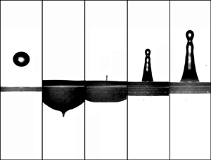
Figure 1. Sequence of images showing the impact of a water drop of radius  $R_d$ falling on a deep liquid pool with a velocity $V$ such that $We=\rho V^2 R_d/\sigma \simeq 90$, $Fr=V^2/(g R_d)=565$, with $g$,
$g$,  $\rho$ and $\sigma$ being the gravitational acceleration, the density and the interfacial tension coefficient, respectively, at different instants of time $T$, with $T=0$ the instant the drop touches the surface: (a) $t=T V/R_d\simeq -2.3$ (b) $T V/R_d\simeq 41$, (c) $T V/R_d\simeq 46$, (d) $T V/R_d\simeq 57$, (e) $T V/R_d\simeq 68.7$. The value of $We$ has been calculated using the material properties of water. In this experiment, the thin jet initially observed in $(\textit {c})$ breaks into tiny droplets and widens with time.
Indeed, the high-speed jets formed after the bursting of bubbles (MacIntyre Reference MacIntyre1972; Duchemin et al. Reference Duchemin, Popinet, Josserand and Zaleski2002; Ghabache et al. Reference Ghabache, Antkowiak, Josserand and Seon2014) or after a drop impacts a free surface (Prosperetti, Crum & Pumphrey Reference Prosperetti, Crum and Pumphrey1989; Prosperetti & Oguz Reference Prosperetti and Oguz1993; Rein Reference Rein1996; Ray, Biswas & Sharma Reference Ray, Biswas and Sharma2015; Michon et al. Reference Michon, Josserand and Séon2017; Thoroddsen et al. Reference Thoroddsen, Takehara, Nguyen and Etoh2018; Yang, Tian & Thoroddsen Reference Yang, Tian and Thoroddsen2020) share a common feature since they both emerge as a consequence of the axial convergence of the capillary waves that propagate along the collapsing cavity walls. Moreover, the largest jet velocities measured in each of these physical situations are quite similar:  $\sim 50$ m s $^{-1}$ in the case of the collapse of Faraday waves (Zeff et al. Reference Zeff, Kleber, Fineberg and Lathrop2000) or when a drop impacts a deep liquid pool (Thoroddsen et al. Reference Thoroddsen, Takehara, Nguyen and Etoh2018; Yang et al. Reference Yang, Tian and Thoroddsen2020), whereas in the case of bubble bursting jets, Blanco-Rodríguez & Gordillo (Reference Blanco-Rodríguez and Gordillo2020) have reported maximum velocities of $\simeq \sigma /\mu$, with $\sigma$ and $\mu$ respectively indicating the interfacial tension coefficient and the liquid viscosity, which, in the case of water properties, imply maximum jet speeds of $\sim 70$ m s $^{-1}$.
It is the main purpose of this contribution to provide conclusive evidence showing that the velocities of the high-speed, thin jets produced following the bursting of a bubble or after the impact of a drop on a deep liquid pool can be quantified using a common theoretical framework, which has already been put forward in Gordillo & Rodríguez-Rodríguez (Reference Gordillo and Rodríguez-Rodríguez2019), where the flow field is represented as the one produced by a line of sinks. Moreover, the flow rate per unit length and also the length of the line of sinks will be expressed as a function of the initial radius of the crater from which the jet emerges and of the wavelength and velocity of the capillary waves travelling along the cavity walls. The integrals expressing the vertical velocity field can be solved analytically, providing algebraic expressions for the jet velocities as a function of the control parameters of each of the two physical situations at hand. The theoretical velocity fields, as well as the initial jet velocities, will be shown to be in quantitative agreement with both the numerical results and experimental measurements.
The paper is structured as follows: in § 2 the ejections of the jets produced after the bursting of a bubble or after the impact of a drop on a liquid pool are simulated numerically. The velocity fields computed in § 2 are compared with the theoretical predictions in §§ 3 and 4 for the cases of bubble bursting jets and of drops impacting a deep liquid pool, respectively. The main results are summarised in § 5.
2. Numerical simulations
The numerical results in figure 2, which illustrate the generation and propagation of the capillary waves that give rise to the emergence of the jets produced by the bursting of a bubble or by the impact of a drop falling on a deep pool, have been obtained, as well as the rest of numerical results shown in this contribution, using the open-source package GERRIS (Popinet Reference Popinet2003, Reference Popinet2009) assuming that the surrounding gaseous atmosphere is air with a density and a dynamic viscosity of  $1.2$ kg m $^{-3}$ and $1.8\times 10^{-5}\ \textrm {Pa} \cdot \textrm {s}$, respectively.

Figure 2. (a) Sequence of events following the bursting of a bubble at a free interface for  $Oh=0.012$. The retraction of the rim causes capillary waves of wavelength $\lambda ^*\propto Oh^{1/2}$ (Gordillo & Rodríguez-Rodríguez Reference Gordillo and Rodríguez-Rodríguez2019) that propagate along the cavity walls and which, when reaching the base of the void, trigger the formation of a fast jet of an initial velocity $V_{jet}$ and an initial radius $R_{jet}$. The impact of a drop shown in (b), with $Fr=600$, $We=90$ and $Mo=Mo_w$, reveals a similar jet ejection process to that depicted in (a), with the main difference being that the dimensionless radius of the cavity is $r_c\simeq 0.5 Fr^{1/4}$ (Prosperetti & Oguz Reference Prosperetti and Oguz1993; Jain et al. Reference Jain, Jalaal, Lohse and van der Meer2019); see (2.4). Figure (b) also shows that, in contrast with the case of bubble bursting jets, $\lambda ^*\approx 1$.
From now on, dimensionless variables will be written using lower-case letters to differentiate them from their dimensional counterparts, written in capitals, and  $\rho$, $\mu$ and $\sigma$ will denote the liquid density, viscosity and interfacial tension coefficient, respectively. Moreover, the acronyms BB and DP will be used in what follows to indicate variables or results that correspond either to the bursting of a bubble or to the impact of a drop on a liquid pool.
Furthermore, the numerical results that correspond to the bursting of a bubble with a radius  $R_b=(3 \mathcal {V}_b/(4{\rm \pi} ))^{1/3}$, with $\mathcal {V}_b$ indicating the bubble volume, will be presented in terms of dimensionless variables defined using $R_b$, the capillary velocity $\sqrt {\sigma /(\rho R_b)}$ and the capillary pressure $\sigma /R_b$ as the characteristic values of length, velocity and pressure, respectively – see figure 2(a). This physical situation is characterised by two dimensionless parameters; namely, the Bond ( $Bo$) and Ohnesorge ( $Oh$) numbers – or, equivalently, the Bond and Laplace ( $La$) numbers, which are defined as
 \begin{equation} Bo=\frac{\rho g R_b^2}{\sigma}, \quad Oh=\frac{\mu}{\sqrt{\rho R_b \sigma}} \quad\mathrm{with}\ La=\frac{\rho R_b\sigma}{\mu^2}=Oh^{{-}2} . \end{equation}
The Ohnesorge number varies within a range of values  $0.006\leq Oh\leq 0.032$ and, except in the Appendix A, the value of the Bond number is kept constant and equal to $Bo=0.01$.
Figure 2(a) shows that the unperturbed air-liquid interface located far from the bubble is flat, and this horizontal boundary has been used to divide the computational domain into two identical cylinders with a height and radius of 5 dimensionless units. The present numerical simulations reproduce those which have already been published in Brasz et al. (Reference Brasz, Bartlett, Walls, Flynn, Yu and Bird2018), Blanco-Rodríguez & Gordillo (Reference Blanco-Rodríguez and Gordillo2020) and have been carried out by imposing symmetry conditions at the axis and zero flux at the rest of the boundaries. The dynamically adaptive numerical grid has been refined up to a level of 14, which means that each grid cell can be subdivided up to 14 times in order to appropriately describe the flow at those regions with high gradients or large values of the interfacial curvature.
From now on, the results of the simulations that correspond to the impact of a drop with a radius  $R_d$ falling over a pool of the same type of liquid with a velocity $V$ will be expressed in terms of the following dimensionless variables, defined using $R_d$, $V$ and $\rho V^2$ as characteristic values of length, velocity and pressure
 \begin{equation} Fr=\frac{V^2}{g R_d} , \quad We=\frac{\rho V^2 R_d}{\sigma} ,\quad Mo=\frac{g \mu^4}{\rho\sigma^3}, \quad Mo_w=25.74\times 10^{{-}12},\end{equation}
with  $g$ denoting the acceleration of gravity, $Fr$ the Foude number, $We$ the Weber number, $Mo_w$ the value of the Morton number corresponding to the physical properties of water and $Mo$ the Morton number, which is related with the Ohnesorge number based on $R_d$, $Oh_d=\mu /\sqrt {\rho \sigma R_d}$, as:
 \begin{equation} Oh_d=(Mo Fr/We)^{1/4} .\end{equation}
 The leftmost panel in figure 2(b) shows that the drop is initially placed at a distance of 0.04 dimensionless units above the gas-liquid interface. This flat boundary is used to divide the numerical domain into two identical cylinders with a height and a radius of  $N$ dimensionless units, with $N=27$ for $Mo=Mo_w$. The numerical calculations have been performed by imposing a free outflow boundary condition at the top part of the numerical region and free-slip and impermeable boundary conditions at the axis of symmetry and at the lateral and the bottom surfaces of the domain. The maximum grid refinement level varies between 12 and 14, and it was verified that the results obtained for $Fr=600$ replicate those in Ray et al. (Reference Ray, Biswas and Sharma2015). Unless otherwise specified, the value of the Morton number in the simulations presented here correspond to the value of the Morton number $Mo=Mo_w$ given in (2.2a–d). The values of $Fr$ and $We$ explored here are indicated in figure 3, where the two solid lines with equations provided in Prosperetti & Oguz (Reference Prosperetti and Oguz1993) delimit the bubble entrapment region described in Pumphrey, Crum & Bjorno (Reference Pumphrey, Crum and Bjorno1989). In view of (2.3), the fact that $Mo=Mo_w$ does not imply a constant value of $Oh_d$.

Figure 3. The squares and circles in the figure indicate the values of the Froude and Weber numbers used in the simulations for the case of DP jets when  $Mo=Mo_w$ see (2.2a–d). The area limited by the curves $We=18.24 Fr^{0.179}$ and $We=20.35 Fr^{0.247}$ given in Prosperetti & Oguz (Reference Prosperetti and Oguz1993) indicates the bubble entrapment region.
Figure 2 shows that both the BB and DP jets emerge after the capillary waves excited by the rim retraction process reach the base of the cavity with an initial radius  $r_c$. Whereas $r_c=1$ for BB jets, the impact of a drop on a liquid pool produces a crater with a dimensionless radius given by (Prosperetti & Oguz Reference Prosperetti and Oguz1993; Jain et al. Reference Jain, Jalaal, Lohse and van der Meer2019)
 \begin{equation} \mathrm{DP:}\ r_c\simeq 0.5 Fr^{1/4} .\end{equation}
In both the BB and DP cases, capillary waves with a characteristic wavelength  $\lambda ^*$ propagate with a dimensionless velocity $v_\lambda$; see figure 2. Figures 4 and 5 illustrate the way the values of $v_\lambda$ have been determined numerically: the shapes of the cavities are calculated at different instants of time separated at regular intervals ${\rm \Delta} t$ at which the increments in the angular positions of the maximum elevation of the capillary waves, ${\rm \Delta} \theta$, are also determined with the purpose of calculating $v_\lambda$ as
 \begin{equation} v_\lambda=r_c \frac{{\rm \Delta}\theta }{{\rm \Delta} t}.\end{equation}
The results obtained from the analysis, depicted in figure 6, reveal that, for the case of BB jets,  $v_\lambda \simeq 5$, a value which is independent of $Oh$ and which coincides with the one reported in Gordillo & Rodríguez-Rodríguez (Reference Gordillo and Rodríguez-Rodríguez2019). For the case of DP jets, figure 6 represents the velocity of the waves $V_\lambda =V v_\lambda$, with $v_\lambda$ given in (2.5), divided by the capillary velocity based on the radius of the cavity, $\sqrt {\sigma /(\rho R_d 0.5 Fr^{1/4})}$. The result in this figure reveals, also in this case, that the waves propagate with a velocity which is proportional to the capillary velocity based on the radius of the cavity. The proportionality constant, however, varies slightly with $Fr$ and $We$, and it is somewhat smaller than in the case of the BB jets. In the remainder of this contribution, the variations with $Fr$ and $We$ depicted in figure 6 will be neglected, and the speed of the capillary waves will be approximated as $3.5 \sqrt {\sigma /(\rho R_d 0.5 Fr^{1/4})}$; namely, 3.5 times the capillary velocity based on the radius of the deformed cavity.

Figure 4. Time evolution of the capillary waves excited after the bursting of a bubble for  $Bo=0.01$ and $Oh=0.006$ (a), $Oh=0.012$ (b), $Oh=0.020$ (c) and $Oh=0.032$ (d). The shape of the bubble at $t=0.100$ is represented in all figures in black. Notice that the radii of curvature of the travelling capillary waves, which is a proxy for the wavelength, $\lambda ^*$, increase with $Oh$. Here, $z_{fs}$ indicates the vertical position of the flat free interface.

Figure 5. Time evolution of the capillary waves excited after a drop impacts a deep liquid pool for  $Mo=Mo_w$. Top row: $Fr=300$ and $We=60$ (a), $We=75$ (b). Middle row: $Fr=600$ and $We=75$ (c), $We=90$ (d). Bottom row: $Fr=3000$ and $We=90$ (e), $We=120$ (f). The cavity shape at $t=10$ is represented in all figures in black. The radii of the circles in dashed lines are $r_c=0.5 Fr^{1/4}$. Notice that the radii of curvature of the travelling capillary waves do not noticeably change with $Fr$ or $We$ and are similar to those of the impacting drop; namely, $\lambda ^*\approx 1$. Here, $z_{fs}$ indicates the vertical position of the flat free interface.

Figure 6. Propagation velocity of the capillary waves for the cases of (a) BB jets and (b) DP jets. The values represented have been calculated using (2.5), with  ${\rm \Delta} \theta$ obtained from the analysis of figures 4 and 5. The result in figure (a) is the same as the result already reported in Gordillo & Rodríguez-Rodríguez (Reference Gordillo and Rodríguez-Rodríguez2019), where it was found that the velocity of capillary waves is independent of $Oh$ and is equal to five times the capillary velocity based on $R_b$. This result is also valid for arbitrary values of $Bo$; see the Appendix A.
Moreover, it can be seen from figure 4 that the maximum radii of curvature of the capillary waves excited for the case of BB jets, which are a proxy to the wavelength  $\lambda ^*$, increase with $Oh$. This result was already reported in Gordillo & Rodríguez-Rodríguez (Reference Gordillo and Rodríguez-Rodríguez2019), where, in addition, it was predicted and later confirmed from an analysis of the numerical results that $\lambda ^*\propto Oh^{1/2}$. In contrast, in the case of DP jets, the wavelength of the capillary waves is somewhat similar to the initial radius of the drop, which can be noted in figure 5. Therefore, from now on, $\lambda ^*\approx 1$ for the case of DP jets. Notice that the reason for the different scaling for $\lambda ^*$ is due to the fact that, in the case of DP jets, the initial thickness of the retracting rim that induces the generation of the capillary waves that travel along the cavity walls is not negligible, which is in contrast to the case of BB jets (Gordillo & Rodríguez-Rodríguez Reference Gordillo and Rodríguez-Rodríguez2019). Instead, this rim possesses an initial thickness which is similar to the wavelength of the wave that, after the impact, displaces the initially flat interface upwards. This fundamental difference from the case of BB jets is the reason why, for the case of DP jets, $\lambda ^*$ does not scale with the Ohnesorge number based on $r_c=0.5 Fr^{1/4}$. This result is further confirmed in figure 7, where it is shown that $\lambda ^*$ and the wave propagation velocity are insensitive to changes of $Mo$.
$Mo$.

Figure 7. Comparison between the time evolutions of the capillary waves excited after a drop impacts a deep liquid pool at the same values of  $t$ for $Fr=600$, $We=114$ and three different values of $Mo$:
$Mo$:  $Mo_1=1.75 Mo_w$ (dashed line), $Mo_2=16 Mo_1$ (dashed-dotted line) and $Mo_3=81 Mo_1$ (solid line), which implies a threefold variation of $Oh_d=(Mo Fr/We)^{1/4}$. In contrast to the BB case depicted in figure 4, the wavelength of the wave travelling along the cavity walls does not depend on $Mo$ and, thus, it does not depend on $Oh_d$; see (2.3); the velocity of the capillary waves does not depend on $Oh_d$ either. Here, $Mo_w$ indicates the value of the Morton number corresponding to the physical properties of water given in (2.2a–d).
Figure 8 shows a key result for our subsequent purposes: the radial velocities at the base of the deformed cylindrical cavity at the scale  $\sim r_c$ are quite similar to the values of the capillary wave velocities depicted in figure 6, and this result applies to the arbitrary values of $Oh$ for the BB case and of $Fr$,
$Fr$,  $We$ and $Mo$ for DP jets. The main consequence of the fact that the capillary waves propagate at velocities which are clearly larger than the capillary velocity based on the crater radius for both BB and DP jets is that the values of the Weber number based on the wave velocity and on the unperturbed radius of the cavity are $\approx 25$ for the case of BB jets and arbitrary values of $Oh$ and $\gtrsim 10$ for the case of DP jets; see figure 8. Therefore, in both cases, the dynamic pressure associated with the velocities induced by the propagation of the capillary waves is an order of magnitude larger than the capillary pressure, a fact that suggests that the implosion of the base of the cavity and the subsequent ejection of the jet could be described as a purely inertial process in which capillarity plays a subdominant role. Section 4 will be devoted to exploring this possibility; however, before this is done, the computed velocity fields for the case of BB jets will be compared with the ones predicted by the theory in Gordillo & Rodríguez-Rodríguez (Reference Gordillo and Rodríguez-Rodríguez2019).

Figure 8. The radial velocity  $V_r$ at the base of the deformed cavity is very similar to the values of the wave velocities depicted in figure 6; namely, $V_r\simeq V_\lambda$. In this figure, $V_c=\sqrt {\sigma /(\rho R_c)}$, with $R_c=R_b$ for BB jets or $R_c=0.5 R_d Fr^{1/4}$ for DP jets. Since the Weber number based on the wave velocity is such that $(V_\lambda /V_c)^2\simeq (V_r/V_c)^2\gg 1$, the radial collapse of the void that gives rise to the ejection of the jet is driven by inertia, and not by capillarity. Figure (a) shows a BB case with $Oh=0.032$ and (b) shows a DP case with $Fr=600$, $We=90$ and $Mo=Mo_w$.
3. Comparison of the numerical results corresponding to the case of bubble bursting jets with theoretical predictions assuming an inertio-capillary balance
Figure 9 illustrates that the velocity field can be divided into three well-defined spatio-temporal regions: (i) the bulk, with a velocity field  $\boldsymbol {v}(r,z,t)$; (ii) the jet region, which extends along the spatio-temporal region $z_{min}(t)\leq z\leq s(t)$; and (iii) the drop, located at $z=s(t)$. In the limit of low-viscosity liquids of interest here, $Oh\ll 1$ and $Oh_d\ll 1$, see (2.1a,b) and (2.3), vorticity is confined within thin regions located very close to the interface and, therefore, the bulk velocity field is irrotational. The velocity potential $\phi$, with $\boldsymbol {v}(r,z,t)=\boldsymbol {\nabla }\phi$, satisfies the Laplace equation $\nabla ^2\phi =0$. The bulk region ends at $z=z_{min}(t)$; namely, just at the beginning of the jet region, where the equations governing the flow can be notably simplified, as reported recently in Blanco-Rodríguez & Gordillo (Reference Blanco-Rodríguez and Gordillo2020). Indeed, due to the fact that the jet geometry is slender and the dynamic pressure is much larger than the capillary pressure since, otherwise, a jet would not be formed (Gordillo & Rodríguez-Rodríguez Reference Gordillo and Rodríguez-Rodríguez2019), pressure gradients within the jet can be neglected and, therefore, the vertical momentum equation for $u(z,t)$ reduces to $\textrm {D}u/\textrm {D}t=0$, with $\textrm {D}/\textrm {D}t$ indicating the material derivative. This momentum equation indicates that the flow within the jet is ballistic; namely, that fluid particles conserve the velocities they possess at the base of the jet. These velocities are prescribed by $\boldsymbol {v}$ since $u(z=z_{min}(t),t)=v_z(r=0,z=z_{min}(t),t)$, where $v_z$ indicates the vertical component of the bulk velocity field. As explained in Blanco-Rodríguez & Gordillo (Reference Blanco-Rodríguez and Gordillo2020), the time evolution of the radius of the drop, $b(t)$, and of the jet tip velocity, $v_{tip}(t)$, can be determined by applying integral balances of mass and momentum at $z=s(t)$ once the functions $u(z,t)$ and $\chi (z,t)$, calculated using the method described in Gekle & Gordillo (Reference Gekle and Gordillo2010), are particularised at $z=s(t)$; see figure 9. Moreover, the criterion derived in Blanco-Rodríguez & Gordillo (Reference Blanco-Rodríguez and Gordillo2020) determines the instant $t^*$ at which the drop detaches from the jet and, hence, the drop radius and velocity can be predicted as $v_d=v_{tip}(t^*)$, $r_d=b(t^*)$.

Figure 9. Sketch showing the meaning of the different variables used to characterise the jet ejection process as well as the different spatio-temporal regions in which the flow can be divided; namely, the bulk, jet and drop regions. These variables are defined in the main text, except for the jet radius  $r_j$ and the velocity $v_j$ at the spatio-temporal boundary where the jet meets the drop: $r_j(t)=\chi (z=s(t),t)$, $v_j(t)=u(z=s(t),t)$, with $ds/\textrm {d} t=v_{tip}(t)$ and $v_{tip}(t)$ and $b(t)$ calculated using integral balances of mass and momentum, while $u(z,t)$ and $\chi (z,t)$ are calculated using the method of characteristics described in Gekle & Gordillo (Reference Gekle and Gordillo2010); see also Blanco-Rodríguez & Gordillo (Reference Blanco-Rodríguez and Gordillo2020), where the integral balances of mass and momentum at the drop are solved. The decomposition of the flow in three regions and the very good agreement between the predictions and the numerical results presented in Blanco-Rodríguez & Gordillo (Reference Blanco-Rodríguez and Gordillo2020) reveal that the jet is driven by the bulk velocity field $\boldsymbol {v}$: once the value of the bulk velocity field is known at the base of the jet, both the spatio-temporal evolution of the jet and the drop radius and velocity can be predicted using the equations in Gekle & Gordillo (Reference Gekle and Gordillo2010), Blanco-Rodríguez & Gordillo (Reference Blanco-Rodríguez and Gordillo2020).
Figure 9, together with the explanations given above, reveal that once  $\boldsymbol {v}$ is known, the functions describing the jet radius and velocity $\chi (z,t)$ and $u(z,t)$, the jet tip radius and velocity $b(t)$ and $v_{tip}(t)$, and even the drop radius and velocity $r_d$ and $v_d$, can be calculated as a function of the control parameters using the results described in Blanco-Rodríguez & Gordillo (Reference Blanco-Rodríguez and Gordillo2020). Since our main interest is in describing the origin of the jets, this section focuses on providing analytical expressions for the irrotational bulk velocity field $\boldsymbol {v}(r,z,t)$, and special attention is paid to the value of $v_z$ at $r=0$ and $z=z_{min}(t')$, with $t'$ the instant at which the minimum value of $r_{min}(t)$ is attained; see figures 9 and 10. With that purpose in mind, it proves convenient to now define $z_{jet}=z_{min}(t')$, $r_{jet}=r_{min}(t')$, and also $v_{jet}=v_z(r=0,z_{jet},t')$, which represents the vertical component of the bulk velocity at the axis when the radius of the base of the collapsing cavity is the minimum. The relevance of $v_{jet}$ can be understood because this is the maximum velocity with which the liquid flows into the jet and, thus, at the usual limit at which the capillary force pulling back the tip of the jet is small compared with inertial terms in the momentum balance, $v_{tip}(t)\simeq v_{jet}$ and $v_d\simeq v_{jet}$: this is due to the fact that material points conserve their velocities when flowing along the jet and because the jet tip barely decelerates through capillary forces at the usual limit when the dynamic pressure is much larger than the capillary pressure. As shown by the results reported in Blanco-Rodríguez & Gordillo (Reference Blanco-Rodríguez and Gordillo2020), the capillary forces pulling the tip of the jet downwards will make $v_d < v_{jet}$, but it will be shown here that these differences are small for low values of the Ohnesorge number.

Figure 10. Panel (a) is a sketch representing the base of the cavity from which the jet is ejected, and panel (b) indicates that the velocity field can be approximated by a line of sinks with intensities  $\textrm {d} Q(z_0)=-2 {\rm \pi}q(z_0)\,\textrm {d} z_0$ extending along the axis of symmetry a distance proportional to the wavelength $\lambda ^*\propto Oh^{1/2}$ (see figures 2a and 4).
In summary, in this contribution the values of  $v_{jet}$ and $v_d$ will be reported, but those of the velocity field $u(z,t)$ will not – see figure 9 – which, in contrast, could be calculated using the theoretical framework presented in Blanco-Rodríguez & Gordillo (Reference Blanco-Rodríguez and Gordillo2020). Moreover, this contribution will focus on the description of bubble-bursting jets in the range $Oh\leq 0.02$, for which a bubble is not entrapped before the jet is produced and for which $v_d\simeq v_{jet}$. The cases corresponding to the ejection of jets after a bubble is entrapped for $0.02 < Oh < 0.04$, which has been studied carefully in Blanco-Rodríguez & Gordillo (Reference Blanco-Rodríguez and Gordillo2020), reveal that the capillary deceleration at the tip of the jet can no longer be neglected and, as a consequence of this, $v_d$ is noticeably smaller than $v_{jet}$.
Recalling now that the dimensionless variables in this section are defined using  $R_b$, the capillary velocity $\sqrt {\sigma /(\rho R_b)}$ and the capillary pressure $\sigma /R_b$ as the characteristic values of length, velocity and pressure, respectively, our analysis starts by noticing that Gordillo & Rodríguez-Rodríguez (Reference Gordillo and Rodríguez-Rodríguez2019) reported that the bulk velocity field $\boldsymbol {v}$ giving rise to BB jets – see figure 9 – can be calculated as the velocity field produced by a line of sinks of length $\ell$ and intensity $q(z)$, with $\ell \propto \lambda ^*\propto Oh^{1/2}$, $\lambda ^*$ the characteristic wavelength of the waves travelling along the cavity walls and $q(z)$ the flow rate per unit length induced by the collapse of the void with a radius
 \begin{equation} h(z)=z\tan \beta ,\end{equation}
with  $\beta$ the opening semiangle of the truncated cone from which the jet is ejected (see figure 10a). The flow rate induced by the sinks located at a vertical position $z_0$ can thus be calculated as (see figure 10b)
 \begin{equation} \textrm{d}Q(z_0)={-}2{\rm \pi} q(z_0) \, \textrm{d} z_0={-}2{\rm \pi} h(z_0) v_r(z_0)\,\textrm{d} z_0,\end{equation}
with  $v_r$ calculated from the balance between the inertial and capillary terms in the Euler-Bernoulli equation (Zeff et al. Reference Zeff, Kleber, Fineberg and Lathrop2000; Sierou & Lister Reference Sierou and Lister2004; Lai et al. Reference Lai, Eggers and Deike2018),
 \begin{equation} v_r\propto (\cos\beta)^{1/2}h^{{-}1/2}.\end{equation}
The substitution of (3.1) and (3.3) into (3.2) yields
 \begin{equation} \textrm{d} Q(z_0)={-}2{\rm \pi} Kz_0^{1/2}\sqrt{\sin\beta} \,\textrm{d}z_0, \end{equation}
with  $K$ the proportionality constant arising from the balance in (3.3). Therefore, the velocity field at $(z,\epsilon )$ (see figure 10) generated by a line of sinks of length $\ell$ extending from $z=z_s=z_{min}+\alpha r_{min}$ to $z=z_s+\ell$, with $\alpha$ an order unity constant, independent of time, and $r_{min}(t)$ and $z_{min}(t)=r_{min}(t)/\tan \beta$ indicating the radial and vertical coordinates of the base of the cavity (see figure 10) can be expressed as
 \begin{equation} \boldsymbol{v}(z,\epsilon)=\frac{1}{4 {\rm \pi}} \int_{z_s}^{z_s+\ell}\frac{\epsilon \boldsymbol{e}_{r} +(z-z_0)\boldsymbol{e}_{z}}{[(z-z_0)^2+\epsilon^2]^{3/2}}\,\textrm{d} Q(z_0),\end{equation}
with  $\boldsymbol {e}_r$ and $\boldsymbol {e}_z$ indicating the unit vectors in the radial and axial directions, respectively.
The substitution of (3.4) into (3.5) yields the following expressions for the vertical and radial components of the velocity:
 \begin{equation} v_z(z,\epsilon)=\frac{-K \sqrt{\sin\beta}}{2} \int_{z_s}^{z_s+\ell}\frac{z_0^{1/2}(z-z_0)}{[(z-z_0)^2 +\epsilon^2]^{3/2}}\,\textrm{d} z_0,\end{equation}
and
 \begin{equation} v_r(z,\epsilon)=\frac{-K \sqrt{\sin\beta}}{2} \int_{z_s}^{z_s+\ell}\frac{z_0^{1/2} \epsilon}{[(z-z_0)^2 +\epsilon^2]^{3/2}}\,\textrm{d} z_0 . \end{equation}
 Equations (3.6) and (3.7) depend on  $\ell$ and also on the constants $\alpha$ and $K$, which are to be determined in what follows. First, the result in Gordillo & Rodríguez-Rodríguez (Reference Gordillo and Rodríguez-Rodríguez2019) is used, where it was reported that the length of the line of sinks $\ell$ is proportional to the wavelength of the capillary waves that trigger the ejection of the jet and, therefore, $\ell \propto \lambda ^*\propto Oh^{1/2}$. Moreover, notice that the integration limits in (3.6) and (3.7) can be expressed as (see figure 10):
 \begin{align} z_s(t)=r_{min}(t)/\tan\beta+\alpha r_{min}(t)\quad\mathrm{and}\quad z_s(t)+\ell=r_{min}(t)/\tan\beta+\alpha r_{min}(t)+\ell, \end{align}
with  $\beta ={\rm \pi} /4$ the opening semiangle of the truncated cone, $\ell \approx Oh^{1/2}$ and $r_{min}(t,Oh)$ indicating the radius of the base of the cavity from which the jet emerges, which is a time-varying quantity, and is not to be confused with $r_{jet}$, which only depends on $Oh$. Indeed, let it be insisted that the maximum jet velocity, $v_{jet}(Oh)$, is reached at the axis of symmetry when the radius of the truncated cone is $r_{jet}(Oh)$, with $r_{jet}$ indicating the minimum value of $r_{min}(t,Oh)$. For $Oh\lesssim 0.03$, Blanco-Rodríguez & Gordillo (Reference Blanco-Rodríguez and Gordillo2020) found that $r_{jet}$ varies linearly with the wavelength of the capillary wave as:
 \begin{equation} r_{jet}=0.2215\left(1-\sqrt{\frac{Oh}{0.0305}}\right), \end{equation}
with the values of the two free constants,  $0.2215$ and $0.0305$, adjusted by fitting the theoretical prediction with the numerical results. For $0.03\lesssim Oh\lesssim 0.04$, a bubble is entrapped before the jet emerges and, in these cases, a viscous cut-off imposes that $r_{jet}\propto Oh^{-2}$ (Gordillo & Rodríguez-Rodríguez Reference Gordillo and Rodríguez-Rodríguez2019; Blanco-Rodríguez & Gordillo Reference Blanco-Rodríguez and Gordillo2020). The role played by viscosity when a bubble is entrapped for $Oh\gtrsim 0.03$ will be clarified in § 4 and, as pointed out above, the focus here will mainly be on the analysis of the jets produced within the range of values of $Oh$ for which no bubbles are entrapped and, thus, (3.9) provides the value of $r_{jet}(Oh)$.
In order to determine the values of the constants  $K$ and $\alpha$, the results in Duchemin et al. (Reference Duchemin, Popinet, Josserand and Zaleski2002) and Lai et al. (Reference Lai, Eggers and Deike2018) are used, where it is found that the time evolution of the jets can be described assuming the inertio-capillary balance, implying that lengths vary in time as $\tau ^{2/3}$, with $\tau$ the instant to or from the ejection of the jet and, therefore, the velocities scale as $\tau ^{-1/3}$. Under this hypothesis, the value of the local Weber number, defined as $We_{local}=r_s(t) v_s^2(t)$ with $r_s(t)\propto r_{min}(t)$ the radial position of a point on the interface and $v_s(t)$ the corresponding liquid velocity, remains constant in time. From the results in figures 6 and 8 in § 2, where it is shown that capillary waves travel at a velocity which is five times the capillary velocity, it is deduced that the value of the local Weber number should be $(V_\lambda /V_c)^2=v^2_\lambda \simeq 25$. Indeed, figure 11 reveals that the value of the local Weber number for $La=Oh^{-2}=4000$ at the point on the interface located at $r_s=1.25 r_{min}$ is roughly constant in time and equal to 25; a similar result is obtained for other values of $r_s$ provided that $r_s/r_{min}<1.5$. Then, the values of the two free constants, $K$ and $\alpha$, are determined from the following two conditions: (i) $We_{local}=25$ at the point on the interface located at $r_s=1.25 r_{jet}(Oh=La^{-1/2}=4000^{-1/2})$, with $r_{jet}$ given in (3.9); and (ii) $v_z(r=0,z=r_{jet}/\tan \beta ,Oh=La^{-1/2}=4000^{-1/2})=v_{jet}(Oh=La^{-1/2}=4000^{-1/2})$, with $v_{jet}$ calculated numerically and $v_z$ calculated by means of (3.6). The solutions to these two equations yield the following values for the two free constants: $K=11.3$ and $\alpha =0.6$.

Figure 11. Comparison between the numerical and the velocity fields calculated using (3.6) and (3.7) for  $\alpha = 0.6$ and $\ell =Oh^{1/2}$, $K=11.3$ and $\beta = {\rm \pi}/4$ for the case of BB jets and $Oh=La^{-1/2}=4000^{-1/2}$. The comparison of the velocity fields on the bottom line correspond to the three jet shapes represented in blue in the top-left image. The red arrows indicate numerical results, whereas the black ones correspond to those computed using (3.6) and (3.7). The black line at the axis indicates where the line of sinks is located.
Figures 12 and 13 show that the velocity field predicted by (3.6) and (3.7) with  $\ell =1.24 Oh^{1/2}$, $K=11.3$ and $\alpha =0.6$ for arbitrary values of $Oh$ are in good agreement with the numerical results at different instants of time after the jet is ejected. Here, the value of the free constant relating the length of the sinks with the wavelength of the capillary wave in $\ell \propto \lambda ^*\propto Oh^{1/2}$ has been set to 1.24 (Gordillo & Rodríguez-Rodríguez Reference Gordillo and Rodríguez-Rodríguez2019): it was checked that the modification of this multiplicative constant between 1 and 1.5 only has a noticeable effect on the velocity fields calculated for $Oh\lesssim 0.01$.

Figure 12. Comparison between the numerical and the analytical velocity fields calculated from (3.6) and (3.7) for  $\alpha = 0.6$, $\ell =1.24 Oh^{1/2}$, $\beta ={\rm \pi} /4$ and $K=11.3$ for the case of BB jets at the different instants of time and different values of $Oh$ corresponding to the bubble shapes depicted in the top row. The red arrows indicate the numerical results, whereas the blue ones correspond to those computed using (3.6) and (3.7). Time advances from top to bottom, the results are grouped in columns and, from left to right, correspond to the following values of the Ohnesorge number: $Oh=La^{-1/2}=27777^{-1/2}$, $Oh=La^{-1/2}=10000^{-1/2}=0.01$ and $Oh=La^{-1/2}=7200^{-1/2}$. The blue line at the axis indicates where the line of sinks is located.

Figure 13. Comparison between the numerical and the analytical velocity fields calculated from (3.6) and (3.7) for  $\alpha = 0.6$, $\ell =1.24 Oh^{1/2}$, $\beta ={\rm \pi} /4$ and $K=11.3$ for the case of BB jets at the different instants of time and different values of $Oh$ corresponding to the bubble shapes depicted in the top row. The red arrows indicate the numerical results, whereas the blue ones correspond to those computed using (3.6) and (3.7). Time advances from top to bottom, the results are grouped in columns and, from left to right, correspond to the following values of the Ohnesorge number: $Oh=La^{-1/2}=4444^{-1/2}$, $Oh=La^{-1/2}=2500^{-1/2}=0.02$ and $Oh=La^{-1/2}=1000^{-1/2}$. The last column corresponds to conditions for which a bubble is entrapped and the fastest jets with the smaller drops are produced (Brasz et al. Reference Brasz, Bartlett, Walls, Flynn, Yu and Bird2018; Blanco-Rodríguez & Gordillo Reference Blanco-Rodríguez and Gordillo2020). The blue line at the axis indicates where the line of sinks is located.
It is noted that the velocity fields calculated using (3.6) and (3.7) depend parametrically on time through  $r_{min}(t)$, which is given by (3.9) only at the instant the jet is ejected. Since figures 12 and 13 show that the velocity fields are accurately predicted by the theory once the jet is ejected, the time evolution of $r_{min}(t)$ could have been calculated using the initial shape of the interface obtained numerically as a starting point, with this shape being updated in time by means of the kinematic boundary condition using the predicted velocity fields. However, the results shown in figures 12 and 13 have been obtained using the values of $r_{min}(t)$ given by the numerical simulations. Notice also that the time evolution of the tip of the jet as well as the drop formation process could be predicted using the velocity fields depicted in figures 12 and 13. As pointed out above, the time evolution of the jets can be described using just the local flow structure near the base of the jet; see Blanco-Rodríguez & Gordillo (Reference Blanco-Rodríguez and Gordillo2020) for details.
Once the values of  $\alpha$, $K$ and $\ell$ are known, the maximum jet velocity can be calculated as $v_{jet}=v_z(r=0,z_{jet}=r_{jet}/\tan \beta )$ with $r_{jet}$ and $v_z$ respectively given in (3.9) and (3.6), which possesses the following analytical solution, already provided in Gordillo & Rodríguez-Rodríguez (Reference Gordillo and Rodríguez-Rodríguez2019):
 \begin{equation} v_{jet}=\frac{K\sin \beta}{2\sqrt{\cos\beta}\sqrt{r_{jet}}} \left[\frac{x_2}{1-x_2^2} - \ln \sqrt{\frac{1+x_2}{1-x_2}} -\frac{x_1}{1-x_1^2} + \ln \sqrt{\frac{1+x_1}{1-x_1}}\right],\end{equation}
where  $x_1^2=z_s/z_{jet}$, $z_s=z_{jet}+\alpha r_{jet}$, $z_{jet}=r_{jet}/\tan \beta$ and $x_2^2=(z_s+\ell )/z_{jet}$, with $\ell =1.24 Oh^{1/2}$, $\alpha = 0.6$, $K=11.3$, $\beta ={\rm \pi} /4$ and $r_{jet}$ given by (3.9).
Figure 14 compares the value of  $v_{jet}(Oh)$ calculated using (3.10) with the numerical values of $v_{jet}$ calculated here and the numerical values of $v_{tip}$ given in Deike et al. (Reference Deike, Ghabache, Liger-Belair, Das, Zaleski, Popinet and Seon2018) – see figure 9 for the definition of $v_{tip}$. Moreover, figure 14 also includes experimental and numerical values that correspond to the velocities of the first drops produced after the breakup of the jet, $v_d$. The results in figure 14 reveal that the predicted values of $v_{jet}$, which are in close agreement with the numerical values, are slightly larger than the velocities of the drops emitted, $v_d$. As explained above, this is a consequence of the capillary deceleration experienced by the tip of the jet, an effect already quantified in Blanco-Rodríguez & Gordillo (Reference Blanco-Rodríguez and Gordillo2020), where a detailed description of the drop formation process is also provided. However, as explained at the beginning of this section, the values of $v_{jet}$ and $v_{tip}$ are very similar to each other within this range of values of $Oh$ because material points move ballistically along the jet and also because of the relatively small deceleration caused by the capillary forces acting on the jet tip.

Figure 14. This figure compares the droplet velocities  $v_d$ for $Bo\leq 0.05$ reported in Ghabache et al. (Reference Ghabache, Antkowiak, Josserand and Seon2014) (green open squares), in Krishnan, Hopfinger & Puthenveettil (Reference Krishnan, Hopfinger and Puthenveettil2017) (purple open triangles), the droplet velocities calculated in Blanco-Rodríguez & Gordillo (Reference Blanco-Rodríguez and Gordillo2020) for $Bo=0.01$ (solid blue dots) and $Bo=0.05$ (solid red dots), the numerical results in figure 6 in Deike et al. (Reference Deike, Ghabache, Liger-Belair, Das, Zaleski, Popinet and Seon2018) for $v_{tip}$, with $v_{tip}$ defined in figure 9 (blue and cyan open symbols, corresponding respectively to $Bo =10^{-3}$ and $10^{-2}$) and also the values for the velocities $v_{jet}$ calculated numerically at $r=0$, $z=z_{jet}=r_{jet}/\tan {\beta }$ when $r_{min}(t)=r_{jet}$ (solid black squares) with the values of $v_{jet}$ (blue continuous line) predicted by (3.10) with $\ell =1.24 Oh^{1/2}$, $\alpha = 0.6$, $K=11.3$, $\beta ={\rm \pi} /4$ and $r_{jet}$ given by (3.9), represented in the inset. Notice that the values of $v_d$ are slightly smaller than $v_{jet}$ as a consequence of the capillary forces pulling the tip of the jet back (Blanco-Rodríguez & Gordillo Reference Blanco-Rodríguez and Gordillo2020).
Equation (3.10) reveals that the origin of the large velocities of the jets produced by bursting bubbles is caused by the combination of two effects: as expressed by (3.9),  $r_{jet}$ decreases with $Oh^{1/2}$ and, therefore, the term $r^{-1/2}_{jet}$ increases with $Oh$. This means that one of the reasons for the large velocities of the jets produced after the bursting of bubbles is that the capillary waves that propagate along the walls of the crater transform the initially rounded cavity into a truncated cone with a radius at its base that is substantially smaller than that of the original bubble. In addition, $v_{jet}$ also increases with $Oh$ because the length of the line of sinks increases as $\propto Oh^{1/2}$. Therefore, the increase in $v_{jet}$ with $Oh$ in the region where no bubbles are entrapped, $Oh\leq 0.02$, is caused by the combination of two effects: $r_{jet}$ decreases with $Oh^{1/2}$, and also because the wavelength of the capillary waves increases with $Oh$ as $\lambda ^*\propto Oh^{1/2}$.
The findings in this section support the results in Gordillo & Rodríguez-Rodríguez (Reference Gordillo and Rodríguez-Rodríguez2019), where the flow field is calculated by being induced by a line of sinks with a length prescribed by the wavelength of the capillary waves, and their flow rate per unit length is fixed by the same inertio-capillary balance as the one which leads to the self-similar solution in Lai et al. (Reference Lai, Eggers and Deike2018), which is proven to be an excellent approximation. Indeed, the self-similar results in Lai et al. (Reference Lai, Eggers and Deike2018) are approximate but not exact because if they were, the value of the local Weber number would not vary in time, whereas figures 11 and 15 show that the value of the local Weber number does experience slight variations in time. This fact is the motivation for the results presented in next section, where whether or not the ejection of BB and DP jets can be described using the theoretical framework in Gordillo & Rodríguez-Rodríguez (Reference Gordillo and Rodríguez-Rodríguez2019) without resorting to the inertio-capillary balance implicitly assumed in (3.3) is explored.

Figure 15. The local Weber number is only approximately constant in time for the case of BB jets. Top and bottom figures correspond, respectively, to  $Oh=0.01$ and $Oh=0.02$.
4. Comparison of the numerical results with predictions relaxing the assumption of an inertio-capillary balance
While the agreement between the predictions and the numerical results in § 3 is fairly good when the intensities of the sinks are calculated using (3.3), this section is devoted to exploring how the predictions of the velocity field are modified when the assumption of an inertio-capillary balance is relaxed.
This discussion begins by noticing that the implosion of a void that is located near a free interface of a low-viscosity liquid such as water shares many similarities with the pinch-off of bubbles which, unlike the case of the pinch-off of drops in air (Eggers Reference Eggers1993; Day, Hinch & Lister Reference Day, Hinch and Lister1998; Burton, Rutledge & Taborek Reference Burton, Rutledge and Taborek2004; Castrejón-Pita et al. Reference Castrejón-Pita, Castrejón-Pita, Thete, Sambath, Hutchings, Hinch, Lister and Basaran2015), is not universal. Indeed, it is well known that the final instants of the collapse of an axisymmetric bubble are not universal because they are strongly dependent on the liquid viscosity (Doshi et al. Reference Doshi, Cohen, Zhang, Siegel, Howell, Basaran and Nagel2003; Suryo, Doshi & Basaran Reference Suryo, Doshi and Basaran2004; Burton, Waldrep & Taborek Reference Burton, Waldrep and Taborek2005; Thoroddsen, Etoh & Takehara Reference Thoroddsen, Etoh and Takehara2007), on the gas flow rate through the neck (Gordillo et al. Reference Gordillo, Sevilla, Rodríguez-Rodríguez and Martínez-Bazán2005) and, most importantly, also on the initial geometry of the cavity, which is characterised, as it is shown in figure 16, by two different length scales,  $r_0$ and $r^{-1}_1$ (Bergmann et al. Reference Bergmann, van der Meer, Stijnman, Sandtke, Prosperetti and Lohse2006; Gordillo & Pérez-Saborid Reference Gordillo and Pérez-Saborid2006). The latter and main difference from the analogous case of the pinch-off of drops in air, together with the slow logarithmic convergence of the system of equations that describe the collapse of a cavity (Gordillo & Pérez-Saborid Reference Gordillo and Pérez-Saborid2006), prevent the purely inertial asymptotic limit being reached. This asymptotic regime is described in Eggers et al. (Reference Eggers, Fontelos, Leppinen and Snoeijer2007), Gordillo & Fontelos (Reference Gordillo and Fontelos2007) but it is never observed in practice (Bolaños Jiménez et al. Reference Bolaños Jiménez, Sevilla, Martínez-Bazán and Gordillo2008; Gordillo Reference Gordillo2008). Therefore, the dynamics governing the final instants of bubble pinch-off do not converge in a real experiment to a universal solution, as it is the case for drops (Eggers Reference Eggers1993; Day et al. Reference Day, Hinch and Lister1998; Burton et al. Reference Burton, Rutledge and Taborek2004; Castrejón-Pita et al. Reference Castrejón-Pita, Castrejón-Pita, Thete, Sambath, Hutchings, Hinch, Lister and Basaran2015), instead needing to be described as solving the system of two ordinary differential equations deduced in Gordillo & Pérez-Saborid (Reference Gordillo and Pérez-Saborid2006), Gordillo (Reference Gordillo2008) for the two lengths, $r_0(t)$ and $r_1^{-1}(t)$, which characterise the time-evolving local shape of the interface $h(z,t)=r_0(t)+z^2 r_1(t)$; see figure 16. These two equations are deduced by making use of the Euler-Bernoulli equation for a time-dependent velocity field generated by a line of sinks of length $\ell _b(t)>r_0(t)$ with $\ell _b\simeq r_0/\sqrt {r_0 r_1}$ (Bergmann et al. Reference Bergmann, van der Meer, Stijnman, Sandtke, Prosperetti and Lohse2006) which, when written in dimensionless variables using, as characteristic values of length, pressure and velocity, an outer length scale $a$, the capillary pressure $\sigma /a$ and the capillary velocity $\sqrt {\sigma /(\rho a)}$ read (Gordillo & Pérez-Saborid Reference Gordillo and Pérez-Saborid2006; Gordillo Reference Gordillo2008):
 \begin{equation} \left.\begin{gathered} \displaystyle\ln(r_0 r_1)\dfrac{\textrm{d} \ln(r_0\dot{r}_0)}{\textrm{d} s}-1 +\gamma\varLambda\dfrac{\hat{p}}{r_0 r_1}+\dfrac{4 Oh}{r_0\dot{r}_0}+\dfrac{2 r_0(1-2 r_0 r_1)}{(r_0\dot{r}_0)^2}=0\\ \displaystyle(\ln(r_0 r_1)+\dfrac{2 Oh}{r_0 \dot{r}_0})\dfrac{\textrm{d} \ln(r_0 r_1)}{\textrm{d} s}-1+\dfrac{\varLambda}{2}\dfrac{p}{r_0 r_1}+\dfrac{4 Oh}{r_0\dot{r}_0}+\dfrac{r_0}{(r_0\dot{r}_0)^2}=0\\ \displaystyle \dfrac{\textrm{d} t}{\textrm{d} s}={-}\dfrac{e^{{-}2s}}{r_0\dot{r}_0} \end{gathered}\right\}. \end{equation}
Figure 16. Sketch showing that the local geometry of a collapsing bubble can be described using a parabola of the type  $h(z,t)=r_0(t)+r_1(t) z^2$. The blue line at the axis indicates the location of the line of sinks.
The solutions for (4.1), the latter of which is deduced from  $\textrm {d} r_0/\textrm {d} t=\dot {r}_0=r_0\dot {r}_0/r_0$, with $\gamma$ an order unity constant and $s=-\ln r_0$, depend on: (i) the initial conditions; (ii) on the Ohnesorge number $Oh=\mu /\sqrt {\rho a \sigma }$; (iii) the gas to liquid density ratio $\varLambda$; and (iv) on the Reynolds number based on the gas material properties through the functions $p$ and $\hat {p}$ that express gas overpressure. The system of equations (4.1) accurately describes the experimental observations, using liquids with different viscosities, bubbles of different diameters and different initial conditions; see Bolaños Jiménez et al. (Reference Bolaños Jiménez, Sevilla, Martínez-Bazán and Gordillo2008) and Bolaños Jiménez et al. (Reference Bolaños Jiménez, Sevilla, Martínez-Bazán, van der Meer and Gordillo2009). It was also shown in Gordillo (Reference Gordillo2008) that (4.1) reproduced the experimental observations reported in Thoroddsen et al. (Reference Thoroddsen, Etoh and Takehara2007) regarding the time evolution of $r_0(t)$ and regarding the formation of tiny satellite bubbles, and also recovered the Stokes limit deduced in Doshi et al. (Reference Doshi, Cohen, Zhang, Siegel, Howell, Basaran and Nagel2003), Suryo et al. (Reference Suryo, Doshi and Basaran2004), as demonstrated by the experiments in Bolaños Jiménez et al. (Reference Bolaños Jiménez, Sevilla, Martínez-Bazán, van der Meer and Gordillo2009).
The ability of (4.1) to reproduce experimental observations is a clear consequence of the correctness of the different approaches made in the modelling, which start by neglecting the vorticity produced at the gas-liquid interface and by expressing the irrotational velocity field as a line of sinks of dimensionless flow rate per unit length  $\propto r_0\dot {r}_0$ placed at the axis of symmetry along a distance $\ell _b\propto r_0/\sqrt {r_0 r_1}$; see figure 16. In fact, the first logarithmic term in (4.1) results from $\ln (r_0/\ell _b)=1/2\ln (r_0 r_1)$ for $\ell _b=r_0/\sqrt {r_0 r_1}>r_0$. The system solution (4.1) in the inviscid limit $Oh\ll 1$ predicts that $r_0\propto \tau ^{\alpha _c}$ with $\tau$ the time to pinch-off and $1/2<\alpha _c<2/3$, a fact indicating that the collapse of bubbles is faster than in the analogous case of the pinch-off of drops, for which the inertio-capillary balance holds; i.e., $r_0\propto \tau ^{2/3}$ (Day et al. Reference Day, Hinch and Lister1998; Duchemin et al. Reference Duchemin, Popinet, Josserand and Zaleski2002; Lai et al. Reference Lai, Eggers and Deike2018).
In order to understand the reasons why the faster dynamics govern the pinch-off of bubbles, it should be noted that if the initial conditions governing the collapse were such that  $r_1\propto r_0^{-1}$ and the capillary terms were not subdominant, $\ell _b=r_0/\sqrt {r_0 r_1}\propto r_0$ and the first logarithmic term in (4.1), $\ln (r_0/\ell _b)$, would be a constant. In this particular case, the axial and radial lengths characterising the local shape of the bubble around its minimum (see figure 16) would scale in the same way, and only the former of the equations in (4.1) would be required to describe the bubble collapse process. Moreover, a self-similar solution of the type $r_0\propto \tau ^{2/3}$ would be obtained, and the value of the local Weber number would remain constant in time. However, as pointed out above, the (4.1) system converges very slowly (logarithmically) to the asymptotic solution (Gordillo & Pérez-Saborid Reference Gordillo and Pérez-Saborid2006); therefore, it retains a memory of the initial conditions, which, in the case at hand, are represented by the capillary waves propagating towards the base of the bubble. These waves will impose an initial value for $\ell _b$ that, in general, will be different from the value $\ell _b\propto r_0$ required for the system to evolve in a self-similar manner and, moreover, capillary terms are subdominant as depicted in figure 8. These facts explain the findings in § 3 in which the numerical solutions are not, strictly speaking, self-similar; indeed, as depicted in figures 11 and also in 15, the local Weber number is not constant in time.
The reason why the bubble collapse proceeds faster than  $r_0\propto \tau ^{2/3}$ can be understood in simple terms because the length of the sinks $\ell _b(t)\propto r_0/\sqrt {r_0 r_1}$ is larger than $r_0(t)$ and, also, the ratio $\ell _b(t)/r_0(t)$ increases in time, a fact meaning that the cavity shape becomes more slender as the cavity collapses (Gordillo et al. Reference Gordillo, Sevilla, Rodríguez-Rodríguez and Martínez-Bazán2005). Clearly, the longer the line of sinks for a given $r_0$ is, the larger the velocities are and the faster the collapse process will be. From the point of view of the equations governing the collapse of cavities, the smaller values of the exponent $\alpha _c$ in $r_0\propto \tau ^{\alpha _c}$ are associated with the larger values of the time-dependent ratio $\ell _b(t)/r_0(t)>1$, which grows in time for the case of bubbles, but remains constant in time for the self-similar case in which the inertio-capillary balance holds, $r_0\propto \tau ^{2/3}$.
The left column in figure 17 shows a comparison between the predicted and the numerical time evolution of the local shapes of the interface for the values  $Fr=600$, $We=95$ within the bubble entrapment region depicted in figure 3. The system (4.1) is integrated in the limit $\varLambda =0$ using, as initial conditions, the values of $r_0(0)$, $\dot {r}_0(0)$ and $r_1(0)$ taken from the simulations, with $x(0)$ indicating the initial value of the generic variable $x$. It should be highlighted that the solution for the system (4.1) largely depends on the initial geometry of the collapsing bubble.

Figure 17. Left-hand column: The top panel shows the comparison between the numerical local shapes of the bubble entrapped in the DP case corresponding to  $Fr=600$, $We=95$, $Mo=Mo_w$ (continuous lines) and the calculated shapes resulting from the integration of the system (4.1) in the limit $\varLambda =0$ (dashed black lines). Below, a comparison between the numerical values of $r_0(t)$ and of $q(t)$ (squares) with the values calculated by integrating the equations in (4.1). Right-hand column: The top panel shows a comparison between the numerical local shapes of the bubble entrapped in the BB case corresponding to $Oh=0.032$ (colour lines) and the shapes predicted by (4.2a,b) (dashed black lines). Below, a comparison between the numerical values of $r_0(t)$ and $q(t)$ (squares) with the values calculated using the equations in (4.2a,b).
Indeed, the solutions for (4.1) in the limits of negligible gas, viscous and capillary effects read (Gordillo Reference Gordillo2008):
 \begin{align} q=r_0\dot{r}_0=\frac{r_0\dot{r}_0(0)}{r_0 r_1(0)}\times e^{-\sqrt{2s-2s(0)+[\ln(r_0 r_1(0))]^2}}, \quad r_0 r_1=e^{-\sqrt{2s-2s(0)+[\ln(r_0 r_1(0))]^2}},\end{align}
which, when expressed in terms of the time to pinch-off  $\tau$, yield to solutions of the type $r_0\propto \tau ^{\alpha _c}$ with $1/2<\alpha _c<2/3$. Indeed,
 \begin{align} r_0\propto \tau^{\alpha_c}\rightarrow q\propto r_0\dot{r}_0\propto \tau^{2\alpha_c-1}\propto r^{2-1/\alpha_c}_0\rightarrow -\ln q\propto (2-1/\alpha_c) s\rightarrow (2-\frac{1}{\alpha_c})=\frac{\textrm{d} \ln q^{{-}1}}{\textrm{d} s},\end{align}
and, therefore:
 \begin{equation} \alpha_c=\frac{1}{2}\left(1-\frac{1}{2}\frac{\textrm{d}\ln q^{{-}1}}{\textrm{d} s}\right)^{{-}1}, \end{equation}
which, in the limit  $\textrm {d} \ln q^{-1}/\textrm {d} s\ll 1$ reads:
 \begin{equation} \alpha_c\simeq \frac{1}{2}\left(1+\frac{1}{2}\frac{\textrm{d} \ln q^{{-}1}}{\textrm{d} s}\right) .\end{equation}
Then, the substitution of the expression of  $q$ in (4.2a,b) into (4.5) yields:
 \begin{equation} \alpha_c=\frac{1}{2}+\frac{1}{4\sqrt{2[s-s(0)]+[\ln(r_0 r_1(0))]^2}}, \end{equation}
which indicates that the exponent  $\alpha _c$ decreases with time and converges very slowly (logarithmically) to $1/2$. Interestingly, (4.6) also reveals that this convergence depends on the initial conditions through the term representing the initial shape of the cavity, $\ln (r_0 r_1(0))$, this being one of the reasons why the different exponents appear in the literature to describe the pinch-off of bubbles (Gordillo Reference Gordillo2008). Therefore, (4.6) predicts that $\alpha _c$ decreases when the slenderness of the initial shape of the cavity increases; i.e., when $[\ln (r_0 r_1(0))]^2$ increases or the entrapped bubble is more elongated.
The collapse of the bubble entrapped in the case of BB jets for  $Oh=1000^{-1/2}\simeq 0.032$ is depicted in figure 17, where the (4.2a,b) solution, which is valid for low-viscosity liquids when the value of the local Weber number is much larger than the unity, is superimposed into the numerical solution, finding an almost perfect match. Figure 17 also shows that, in agreement with (4.2a,b), the sink strength $r_0\dot {r}_0$ decreases in time as $r_0\rightarrow 0$, a fact meaning that the local value of the Reynolds number, given by $Oh^{-1} r_0\dot {r}_0\simeq 30 r_0\dot {r}_0$, also decreases in time. Therefore, viscous effects become relevant when the bubble splits in two and the jet is ejected; this is the reason why, as mentioned above, for $0.04\gtrsim Oh\gtrsim 0.03$ there exists a viscous cut-off and the minimum radius from which the jet emerges is different from zero. Thus, the existence of the viscous cut-off length avoids singular values of the jet velocity (Gordillo & Rodríguez-Rodríguez Reference Gordillo and Rodríguez-Rodríguez2019). In summary, in general, two different length scales are required to describe the time evolution of the shape of a bubble that splits in two. Moreover, if the ratio of these two length scales is not kept constant along the collapse process, self-similarity is lost and solutions of the type $r_0(\tau )\propto \tau ^{\alpha _c}$, with $1/2<\alpha _c<2/3$, will be found, with smaller values of $\alpha _c$; i.e., with larger values of the velocities for the larger values of the ratio $\ell _b/r_0=1/\sqrt {r_0 r_1}$, see figure 16.
Similar ideas to those expressed above are still applicable for the cases in which a cavity collapses without breaking into two parts, as is the case of the jets emerging from the bases of truncated cones considered in § 3 and sketched in figure 10. Indeed, two different length scales,  $r_{min}(t)$ and $\ell _b$, with $r_{min}$ and $\ell _b$ playing the roles of $r_0$ and $r_0/\sqrt {r_0r_1}$ in (4.1), respectively, are also required to describe the collapse of these cavities. Therefore, since $\ell _b$ is imposed by the capillary waves reaching the base of the cavity and, thus, is constant in time, the ratio $\ell _b/r_{min}(t)$ will increase in time and the collapse will be faster than the self-similar collapse $r_{min}\propto \tau ^{2/3}$, which would only take place if $\ell _b(t)/r_{min}(t)$ remained constant in time, as explained above. Moreover, the first logarithmic term in (4.1) corresponds to $\ln (r_{min}/\ell _b)$ (Gordillo Reference Gordillo2008); therefore, the equation describing the time evolution of the minimum radius of the cavity $r_{min}(t)$, which plays the same role as $r_0(t)$ in the equations above, can be written as:
 \begin{equation} \ln\left(\frac{r_{min}}{\ell_b}\right)\frac{\textrm{d} r_{min} \dot{r}_{min}}{\textrm{d}t}+\frac{1}{2} \dot{r}^2_{min}-\frac{1}{r_{min}}=0 . \end{equation}
Defining  $s=-\ln (r_{min}/\ell _b)$ and the intensity of the sinks as $q=r_{min}\dot {r}_{min}$, (4.7) yields:
 \begin{equation} {-}2s\frac{\textrm{d} \ln q}{\textrm{d} s}-1+\frac{2\ell_b e^{{-}s}}{q^2}=0\Rightarrow \frac{\textrm{d}}{\textrm{d} s}\left(s\frac{q^2}{2}+\ell_b e^{{-}s}\right)=0 \end{equation}
and, therefore, the result found in Gordillo et al. (Reference Gordillo, Sevilla, Rodríguez-Rodríguez and Martínez-Bazán2005) is recovered:
 \begin{equation} q=\frac{q(0)}{\sqrt{-\ln(r_{min}/\ell_b)}} \left(s(0)+2\frac{r_{min}(0)-r_{min}}{q^2(0)}\right)^{1/2}\approx \frac{q(0)}{\sqrt{-\ln(r_{min}/\ell_b)}}, \end{equation}
where the initial conditions at  $s(0)\approx 1$ have been imposed, and it has also been taken into account that, as illustrated in figure 8, $r_{min}(0)/q^2(0)\ll 1$.
The expression for the flow rate in (4.9) has been calculated under the assumption that the collapsing cavity is a cylinder instead of a truncated cone and that the Euler-Bernoulli equation is particularised at the plane of symmetry of the cylinder. Therefore, the result in (4.9) is just an approximation whose validity will be checked a posteriori by comparing the predictions with the numerical results. The physical meaning of (4.9) is that the strength of the sinks driving the jet ejection process is not fixed by an inertio-capillary balance at the scale of  $r_{min}(t)$ as in § 3 but by the flow rate $q(0)$ imposed by the capillary waves travelling towards the pole of the bubble at the scale of the initial radius of the cavity; see figure 8. Then, since
 \begin{equation} \textrm{d} Q(z_0)={-}2{\rm \pi} q \,\textrm{d} z_0,\end{equation}
the substitution of (4.10) into (3.5) yields:
 \begin{equation} v_z(z,\epsilon)={-}\frac{q}{2} \int_{z_s}^{z_s+\ell} \frac{(z-z_0)}{[(z-z_0)^2+\epsilon^2]^{3/2}}\,\textrm{d} z_0 , \end{equation}
and
 \begin{equation} v_r(z,\epsilon)={-}\frac{q}{2}\int_{z_s}^{z_s+\ell}\frac{\epsilon}{[ (z-z_0)^2+\epsilon^2]^{3/2}}\,\textrm{d} z_0 ,\end{equation}
with  $q$ the flow rate per unit length in (4.9), which is constant along the vertical direction. In order to express the flow rate per unit length $q$ in (4.11) and (4.12) as a function of the control parameters, it must be taken into account that since capillary waves propagate in the case of BB jets at five times the capillary velocity at the scale of the radius of the cavity $r_c$, $q(0)\simeq v_\lambda r_c\simeq 5$ (see figure 6a). Therefore, assuming that the unknown length $\ell _b$ in (4.9) is the initial radius of the cavity, $\ell _b=r_c=1$, (4.9) reads:
 \begin{equation} q=\frac{q(0)}{\sqrt{-\ln(r_{min}/\ell_b)}}=\frac{5}{\sqrt{-\ln r_{min}}}.\end{equation}
Notice that the approximation for the flow rate per unit length in (4.13) is asymptotically valid in the limit  $r_{min}\ll 1$ regardless of the exact value of the outer length $\ell _b$. This is because, for an arbitrary value of $\ell _b\sim O(1)$, which is a fixed length independent of time, $|\ln r_{min}|\gg |\ln \ell _b|$ and, therefore, $\ln (r_{min}/\ell _b)=\ln r_{min}-\ln \ell _b\simeq \ln r_{min}$.
It should be pointed out that (4.13) expresses that the flow rate of the sinks controlling the jet ejection process is fixed at the scale of the radius of the unperturbed bubble and also that it can be calculated as the product of the velocity of the capillary waves travelling along the cavity walls towards the base of the bubble times the radius of the bubble, with small logarithmic corrections. The integration limits in (4.11) and (4.12),  $z_s=r_{min}/\tan \beta +\alpha r_{min}$ and $z=z_s+\ell$, depend on $\alpha$, which is fixed here to the value found in § 3, $\alpha =0.6$, and also depend on the length of the sinks, $\ell =C Oh^{1/2}$, with $C$ a multiplicative constant. The value $C=2.8$ used here is determined using the condition that the vertical velocity predicted by (4.11) at the axis of symmetry, $v_z(r=0,z=r_{jet}/\tan \beta )$, with $r_{jet}$ given in (3.9), coincides with the numerical value obtained for the smallest value of $Oh$ explored here, $Oh=6\times 10^{-3}$, at the instant of time the vertical velocity is maximum.
The results depicted in figures 18 and 19 show remarkable agreement between the numerical results and the velocity fields calculated through (4.11)–(4.13) using  $\alpha =0.6$, $\ell =2.8 Oh^{1/2}$ and $q$ given by (4.13) for all values of $Oh$ and $t$.
$t$.

Figure 18. Comparison of the numerical and analytical velocity fields calculated using (4.11) and (4.12) for  $\alpha = 0.6$, $\ell =2.8 Oh^{1/2}$ and $q$ given by (4.13) for the case of BB jets at the different instants of time and different values of $Oh$ corresponding to the bubble shapes depicted in the top row. The red arrows indicate the numerical results, whereas the green ones correspond to those computed using (4.11) and (4.12). Time advances from top to bottom, the results are grouped in columns and, from left to right, the results correspond to the following values of the Ohnesorge number: $Oh=La^{-1/2}=27777^{-1/2}$, $Oh=La^{-1/2}=10000^{-1/2}=0.01$ and $Oh=La^{-1/2}=7200^{-1/2}$. The green line at the axis indicates where the line of sinks is located.

Figure 19. Comparison of the numerical and analytical velocity fields calculated from (4.11) and (4.12) for  $\alpha = 0.6$, $\ell =2.8 Oh^{1/2}$ and $q$ given by (4.13) for the case of BB jets at the different instants of time and different values of $Oh$ corresponding to the bubble shapes depicted in the top row. The red arrows indicate the numerical results, whereas the green ones correspond to those computed using (4.11) and (4.12). Time advances from top to bottom, the results are grouped in columns and, from left to right, the results correspond to the following values of the Ohnesorge number: $Oh=La^{-1/2}=4444^{-1/2}$, $Oh=La^{-1/2}=2500^{-1/2}=0.02$ and $Oh=La^{-1/2}=1000^{-1/2}$. The last column corresponds to conditions for which a bubble is entrapped and the fastest jets with the smaller drops are produced (Brasz et al. Reference Brasz, Bartlett, Walls, Flynn, Yu and Bird2018; Blanco-Rodríguez & Gordillo Reference Blanco-Rodríguez and Gordillo2020). The green line at the axis indicates where the line of sinks is located.
As explained at the beginning of § 3, the maximum jet velocity is attained when  $r_{min}(t)=r_{jet}$ with $r_{jet}$ given in (3.9); therefore, $v_{jet}$ can be predicted solving (4.11) particularised at $z=r_{jet}/\tan \beta$, $\epsilon =0$, which yields:
 \begin{equation} v_{jet}=\frac{q}{2}\left(\frac{1}{\alpha r_{jet}}- \frac{1}{\alpha r_{jet}+\ell}\right) .\end{equation}
The substitution of  $\alpha =0.6$, $\ell =2.8 Oh^{1/2}$ and the value of $q$ in (4.13) into (4.14) yields:
 \begin{equation} v_{jet}=\frac{5}{1.2\sqrt{-\ln r_{jet}}}\left(\frac{1}{r_{jet}}-\frac{1}{r_{jet}+4.67 Oh^{1/2}}\right),\end{equation}
with  $r_{jet}$ given in (3.9).
Figure 20 compares the values of  $v_{jet}$ calculated numerically with those predicted by (4.15). The excellent agreement between the predictions, experiments and the numerical results depicted in figure 20 indicate that (4.15) can be used to calculate the initial jet velocity for all ranges of $Oh$ considered here. Notice that (4.15) predicts the jet velocities slightly more accurately than the analogous (3.10) for the smaller values of $Oh$. However, the differences between the two approaches regarding the smaller range of values of $Oh$ is extremely small, which it can be appreciated in figure 21. In fact, the larger differences, albeit also small, between the two approaches are observed for values of $Oh$ for which a bubble is entrapped; see the case of $La=1000$ in figures 13 and 19, where it can be noted that the analysis of § 3 predicts the numerical velocity field for this particular value of $La$ more accurately.

Figure 20. This figure compares the droplet velocities  $v_d$ for $Bo\leq 0.05$ reported in Ghabache et al. (Reference Ghabache, Antkowiak, Josserand and Seon2014) (green open squares), in Krishnan et al. (Reference Krishnan, Hopfinger and Puthenveettil2017) (purple open triangles), the droplet velocities calculated in Blanco-Rodríguez & Gordillo (Reference Blanco-Rodríguez and Gordillo2020) for $Bo=0.01$ (solid blue dots) and $Bo=0.05$ (solid red dots), the numerical results in figure 6 in Deike et al. (Reference Deike, Ghabache, Liger-Belair, Das, Zaleski, Popinet and Seon2018) for $v_{tip}$, with $v_{tip}$ defined in figure 9 (blue and cyan open symbols, corresponding respectively to $Bo =10^{-3}$ and $10^{-2}$) and also the values for the velocities $v_{jet}$ calculated numerically at $r=0$, $z=z_{jet}=r_{jet}/\tan {\beta }$ when $r_{min}(t)=r_{jet}$ (solid black squares) with the values of $v_{jet}$ (green continuous line) predicted by (4.15) with $r_{jet}$ given by (3.9), represented in the inset. It should be noted that the values of $v_d$ are slightly smaller than $v_{jet}$ as a consequence of the capillary forces pulling the tip of the jet back (Blanco-Rodríguez & Gordillo Reference Blanco-Rodríguez and Gordillo2020). The dashed line is proportional to $Oh^{1/2}$. For comparative purposes, the values of $v_{jet}$ predicted by (3.10) with $\ell =1.24 Oh^{1/2}$, $\alpha =0.6$, $K=11.3$, $\beta ={\rm \pi} /4$ are represented by a blue continuous line. Velocities are made dimensionless using the capillary velocity $\sqrt {\sigma /(\rho R_b)}$.

Figure 21. Comparison between the numerical velocity fields (in red) and the analytical velocity fields calculated using either (4.11) and (4.12) for  $\alpha = 0.6$, $\ell =2.8 Oh^{1/2}$ and $q$ given by (4.13) (in green) or (3.6) and (3.7) for $\alpha = 0.6$, $\ell =1.24 Oh^{1/2}$, $\beta ={\rm \pi} /4$ and $K=11.3$ (in blue). The comparison refers to the case of BB jets at different instants of time and values of $Oh$ corresponding to the bubble shapes depicted in the top row. Time advances from top to bottom, the results are grouped in columns and, from left to right, the results correspond to the following values of the Ohnesorge number: $Oh=La^{-1/2}=27777^{-1/2}$, $Oh=La^{-1/2}=10000^{-1/2}=0.01$ and $Oh=La^{-1/2}=7200^{-1/2}$. The green/blue lines at the axis indicate where the line of sinks is located. Velocities are made dimensionless using the capillary velocity $\sqrt {\sigma /(\rho R_b)}$.
The results shown in this section reveal that the agreement between the predictions, numerical results and experiments is as good as the agreement depicted in § 3. Therefore, the velocity field produced by the bursting of bubbles for arbitrary values of  $Oh$ and for times close to the jet ejection instant can be predicted using the theoretical framework put forward in Lai et al. (Reference Lai, Eggers and Deike2018), Gordillo & Rodríguez-Rodríguez (Reference Gordillo and Rodríguez-Rodríguez2019). It should also be noted that the time evolution of the radius and of the jet tip velocity could be quantified in terms of the time-varying local velocity fields depicted in figures 12 and 13 or 18 and 19 during the instants close to the jet ejection instant; specifically, when $r_{min}(t)=r_{jet}$ using the theoretical framework provided in Blanco-Rodríguez & Gordillo (Reference Blanco-Rodríguez and Gordillo2020).
However, the results in figures 18–20 clearly indicate that the ejection of bubble bursting jets can also be described when the inertio-capillary balance is relaxed. Then, because the expressions deduced in this section are simpler than the analogous ones in § 3, because the equations deduced in this section do not depend on the semiangle  $\beta$ illustrated in figure 10 and also because the ejection of the faster DP jets can only be described when the cavity collapse is driven by inertia as will be shown below, from now on the velocity fields of BB and DP jets will be quantified making use of (4.11), (4.12), (4.14) and (4.15). The Appendix A demonstrates that the equations deduced in this section can also be used to describe the ejection of BB jets for arbitrary values of $Bo \hbox{ and } Oh \leq 0.02$. The Appendix A also provides equations that predict the radii of the ejected droplets and also the droplet velocities $v_d$ with a special emphasis on the case of water.
Thanks to the analogy that exists between BB and DP jets, which has already been pointed out in § 2 and illustrated in figures 4 and 5, the results in this section are used to predict the velocity fields and the initial velocities of the jets produced when a drop falls onto a deep liquid pool. Indeed, the flow rate per unit length  $q(0)$ in (4.9) can also be calculated in the case of DP as the product of the velocity of the capillary waves multiplied by the radius of the cavity, $r_c$, as:
 \begin{equation} q(0)=\frac{V_\lambda R_c}{V R_d}=0.5 Fr^{1/4} v_\lambda,\end{equation}
where it has been taken into account that  $r_c=0.5 Fr^{1/4}$ (Prosperetti & Oguz Reference Prosperetti and Oguz1993; Jain et al. Reference Jain, Jalaal, Lohse and van der Meer2019). The results in figure 6(b) indicate that the velocity of the capillary waves can be approximated as:
 \begin{equation} v_\lambda\simeq 3.5(0.5 Fr^{1/4} We)^{{-}1/2}, \end{equation}
and, therefore, the substitution of the result of (4.17) into (4.16) yields:
 \begin{equation} q(0)\simeq 3.5\sqrt{\frac{0.5 Fr^{1/4}}{We}} .\end{equation}
Consequently, the flow rate per unit length of the sinks that describe the ejection of DP jets can be expressed, using the results in (4.9) and (4.18) as:
 \begin{equation} q\simeq 3.5\sqrt{\frac{0.5 Fr^{1/4}}{-We\ln(2 r_{min} Fr^{{-}1/4})}}, \end{equation}
where  $\ell _b$ is also taken here as the radius of the cavity, $\ell _b=r_c=0.5 Fr^{1/4}$. The same comment made in the case of BB jets applies here: (4.19) is expected to provide an approximate value for the flow rate per unit length $q$ whenever $r_{min}\ll \ell _b\simeq r_c$. Another difference with the case of BB jets is that, in the case of DP jets, $\lambda ^*\approx 1$; see figure 5, and, therefore, (4.11) and (4.12) are solved using $\ell =1$ and $\alpha =0.6$, with $q$ calculated through (4.19). The results, depicted in figures 22–24 for $Mo=Mo_w$, for the ranges of $Fr$,
$Fr$,  $We$ indicated in figure 3 and several instants of time after the jet is issued indicate that, BB and DP jets can indeed be described in terms of the same physical ideas using the theoretical framework presented in Gordillo & Rodríguez-Rodríguez (Reference Gordillo and Rodríguez-Rodríguez2019).

Figure 22. Comparison between the numerical and analytical velocity fields calculated from (4.11) and (4.12) for  $Fr=100$, $Mo=Mo_w$, $\alpha = 0.6$, $\ell =1$ and $q$ given by (4.19) for the case of DB jets at the different instants of time and different values of $We$ that correspond to the bubble shapes depicted in the top row. The red arrows indicate the numerical results, whereas the green ones correspond to those computed using (4.11) and (4.12). Time advances from top to bottom, the results are grouped in columns and, from left to right, the results correspond to the following values of the Weber number: $We=45$, $We=53$, $We=62$. The green line at the axis indicates where the line of sinks is located.

Figure 23. Comparison between the numerical and analytical velocity fields calculated from (4.11) and (4.12) for  $Fr=300$, $Mo=Mo_w$, $\alpha = 0.6$, $\ell =1$ and $q$ given by (4.19) for the case of DB jets at the different instants of time and different values of $We$ that correspond to the bubble shapes depicted in the top row. The red arrows indicate the numerical results, whereas the green ones correspond to those computed using (4.11) and (4.12). Time advances from top to bottom, the results are grouped in columns and, from left to right, the results correspond to the following values of the Weber number: $We=55$, $We=70$, $We=85$. The green line at the axis indicates where the line of sinks is located.

Figure 24. Comparison between the numerical and the analytical velocity fields calculated from (4.11) and (4.12) for  $Fr=600$, $Mo=Mo_w$, $\alpha = 0.6$, $\ell =1$ and $q$ given by (4.19) for the case of DB jets at the different instants of time and different values of $We$ corresponding to the bubble shapes depicted in the top row. The red arrows indicates numerical results, whereas the green ones correspond to those computed using (4.11) and (4.12). Time advances from top to bottom, the results are grouped in columns and, from left to right, the results correspond to the following values of the Weber number: $We=60$, $We=75$, $We=99$. The green line at the axis indicates where the line of sinks is located.
The initial velocity of DP jets can also be predicted by making use of (4.14), which, using the expression of  $q$ given in (4.19), reads:
 \begin{equation} v_{jet}=\frac{3.5}{2}\sqrt{\frac{0.5Fr^{1/4}}{- We\ln(2 r_{jet} Fr^{{-}1/4})}} \times \left(\frac{1}{\alpha r_{jet}}-\frac{1}{\alpha r_{jet}+1}\right),\end{equation}
with  $\alpha =0.6$ and where it has been taken into account that $\lambda ^*=1$ and also that, in this case, variables are made dimensionless using $R_d$, $V$ and $\rho V^2$ as characteristic values of length, velocity and pressure.
The predictions of (4.20) are expected to explain the measured experimental values of the velocities of the very fast jets ejected after the impact of a drop on a liquid pool (Michon et al. Reference Michon, Josserand and Séon2017; Thoroddsen et al. Reference Thoroddsen, Takehara, Nguyen and Etoh2018). Indeed, (4.20) reveals that  $V_{jet}=V v_{jet}$ diverges when $r_{jet}\rightarrow 0$ as $v_{jet}\propto (r_{jet} \sqrt {-\ln r_{jet}})^{-1}$ and, hence, in comparison with the case of bubble bursting jets, extremely fast jets can be ejected if the capillary waves travelling along the cavity walls deform the base of the void in such a way that $r_{jet}\ll 1$. However, in contrast to the case of bubble bursting jets, this type of event happens under very specific values of the control parameters and it is barely repeatable (Michon et al. Reference Michon, Josserand and Séon2017) because the collapsing cavity caused by an impacting drop easily losses axisymmetry, resulting in a reduction in the jet velocity (Gekle & Gordillo Reference Gekle and Gordillo2010). In spite of the fact that these are very rare events, Thoroddsen et al. (Reference Thoroddsen, Takehara, Nguyen and Etoh2018) and Yang et al. (Reference Yang, Tian and Thoroddsen2020) report experiments on DP jets with velocities up to $\simeq 48$ m ${\rm s}^{-1}$, which can be depicted in figure 25, where the experimental measurements are compared with the jet velocities calculated as $V_{jet}=V v_{jet}$, with $v_{jet}$ given by (4.20) and $r_{jet}$ measured from the experimental images included in the figure. It can be seen in figure 25 that the predicted velocity of the jets are, in some cases, in very close agreement with the measured values. It is particularly interesting to note that the fastest velocities reported by Thoroddsen et al. (Reference Thoroddsen, Takehara, Nguyen and Etoh2018) are very well predicted by (4.20). For the other cases depicted in figure 25, the predicted value is close but below the measured value. The reason why the agreement is not equally good for all the cases shown is because the predicted jet velocity depends on $r_{jet}$, which is taken from the images inserted into figure 25, which admit a relative error in the measurements from the pictures provided in Thoroddsen et al. (Reference Thoroddsen, Takehara, Nguyen and Etoh2018) and Yang et al. (Reference Yang, Tian and Thoroddsen2020) of $\pm 20\,\%$. Therefore, the predicted jet velocity depends highly on the instant at which those images were taken. Thus, if the image corresponds to an instant shortly before the jet is issued, $r_{jet}$ in (4.20) will be larger and the calculated value of the velocity $v_{jet}$ will be smaller. This fact explains the different degrees of agreement between the measurements and predictions in figure 25. It should be pointed out that the images in figure 25 that correspond to the experiments in Thoroddsen et al. (Reference Thoroddsen, Takehara, Nguyen and Etoh2018) reflect the instant at which the jet is issued, as explained in the original paper. Notice the close agreement between the predicted and the experimental values for the jet velocity, which is also pretty close to the measured vertical velocities before the jet emerges in figure 6 in Thoroddsen et al. (Reference Thoroddsen, Takehara, Nguyen and Etoh2018). Moreover, in their figures 5 and 6, Thoroddsen et al. (Reference Thoroddsen, Takehara, Nguyen and Etoh2018) provide the value of the exponent $\alpha _c\simeq 0.53\pm 0.02$ in $r_{min}\propto \tau ^{\alpha _c}$ when the collapse of the cavity gives rise to the emergence of jets with velocities of $\sim 50$ m s $^{-1}$ and a bubble is not entrapped. Under these conditions, $r_{min}/r_c=2 r_{min} Fr^{-1/4}\simeq 4\times 10^{-3}\rightarrow s=-\ln (r_{min}/r_c)\simeq 5.5$ during the final instants of time of the radial collapse before the jet emerges. In the present theoretical description, the flow rate per unit length of the sinks that induce the collapse of the cavity and the emergence of the jet given by (4.9) is such that $q^{-1}\propto \sqrt {s}$ and, therefore, (4.5) predicts that:
 \begin{equation} \alpha_c=\frac{1}{2}+\frac{1}{8s}\simeq 0.522, \end{equation}
a value which is quite close to the one measured experimentally. Notice that the values of the exponents predicted by (4.21) are smaller than those in (4.6) that correspond to the case of jets being ejected after a bubble has been entrapped. As pointed out above, the exponent  $\alpha _c$ depends highly on the slenderness of the entrapped bubble as (4.6) clearly shows: the more elongated the entrapped bubble is, the smaller $\alpha _c$ is. These conclusions are in agreement with the results shown in figures 5 and 6 in Thoroddsen et al. (Reference Thoroddsen, Takehara, Nguyen and Etoh2018). Clearly, since the length of the line of sinks $\ell _b$ is constant in time for the case of the jets ejected when a bubble is not entrapped, the ratio $\ell _b/r_{min}$ is larger than in the case where a bubble is entrapped, which explains why the value of the exponent (4.21) calculated using (4.5) is smaller than the value provided in (4.6) for the case where a bubble is entrapped.

Figure 25. Comparison between the experimental measurements in Thoroddsen et al. (Reference Thoroddsen, Takehara, Nguyen and Etoh2018) (in red) and Yang et al. (Reference Yang, Tian and Thoroddsen2020) (in blue) with the jet velocity calculated as  $V_{jet}=V v_{jet}$, with $v_{jet}$ given by (4.20) and $r_{jet}$ measured from the experimental images in the figure. The experimental values of $r_{jet}$ are indicated in red in each of the insets and the black scale bar indicates $5\times 10^{-4}$ m for the experiments in Thoroddsen et al. (Reference Thoroddsen, Takehara, Nguyen and Etoh2018) and $2\times 10^{-4}$ m for the experiments in Yang et al. (Reference Yang, Tian and Thoroddsen2020). In the case of the experiments in Yang et al. (Reference Yang, Tian and Thoroddsen2020), the jet velocity is calculated using the material properties of water. The velocities of the jets produced when a bubble is entrapped in Thoroddsen et al. (Reference Thoroddsen, Takehara, Nguyen and Etoh2018) are taken as that of the downward jets in their figure 4 because the velocities of the upward jets, once they are seen above the free interface, are much smaller as a consequence of the jet tip deceleration caused by the capillary retraction and by the air drag force (Blanco-Rodríguez & Gordillo Reference Blanco-Rodríguez and Gordillo2020).
It should be pointed out that, in contrast with the case of BB jets, which could be equally well described using either the approximation described in this section or the one in § 3, the velocities of the jets produced in the DP case can only be accurately predicted using the results in this section. Indeed, if the inertio-capillary balance were to be preserved during the cavity collapse process, the value of the exponent would be  $\alpha _c=2/3$ and not slightly larger than 0.5 as seen in (4.21), a conclusion which had already been emphasised by Thoroddsen et al. (Reference Thoroddsen, Takehara, Nguyen and Etoh2018) and Yang et al. (Reference Yang, Tian and Thoroddsen2020). Therefore, if the results in § 3 were applied to describe the jet ejection process in the DP case, the jet velocities predicted would be far smaller than those observed experimentally, a conclusion which can also be deduced by comparing (3.10) and (4.20): while in the former case $v_{jet}\propto r^{-1/2}_{jet}$, the values of $v_{jet}$ predicted by (4.20), which are in good agreement with the experimental measurements in figure 25, diverge as $v_{jet}\propto (r_{jet} \sqrt {-\ln r_{jet}})^{-1}\gg r^{-1/2}_{jet}$ when $r_{jet}\rightarrow 0$. Nonetheless, as discussed in the Appendix A, where the effect of the Bond number on the bursting of bubbles is also analysed, jet velocities do not diverge to infinity because $r_{jet}>0$ and, hence, $v_{jet}$ is finite. In this regard, it can be noted that the base of the truncated cone from which the jet is issued shrinks in the axial direction faster than in the radial direction by a factor of $1/\alpha =1/0.6>1$; see (4.14) and (4.20). Therefore, the length of a cylinder with an aspect ratio $\sim 1$ will shrink to zero before its radius is zero, thus preventing the appearance of infinite velocities. This is a purely irrotational mechanism that also avoids the existence of infinite jet velocities.
The case of the much slower and much thicker jets appearing outside the bubble entrapment region depicted in figure 3 is analysed by making use of the experimental data in Michon et al. (Reference Michon, Josserand and Séon2017). Indeed, Michon et al. (Reference Michon, Josserand and Séon2017) report experiments on the velocities and the diameters of the drops emitted from the tip of of DP jets formed with liquids of different viscosities,  $Mo\geq Mo_w$, $We/Fr\simeq 1/4$ and values of the Foude number $200 \lesssim Fr\lesssim 2000$. The radii $r_d$ of the droplets formed under these conditions, which are a good proxy of $r_{jet}$ because, for this range of values of $Fr$ and $We$, the jets are mostly cylindrical, are provided in figure 4(b) of Michon et al. (Reference Michon, Josserand and Séon2017) for $Mo=Mo_w$. The jet velocities calculated by means of (4.20) when $r_{jet}$ is approximated linearly to the data for $r_d$ in Michon et al. (Reference Michon, Josserand and Séon2017) are compared with the experimental results in figure 26(b), where it can be seen that, in spite of approximating $r_{jet}$ by $r_d$, the predicted jet velocity is in fair agreement with experiments. Figure 26 also shows that the experimental results deviate from the scaling proposed in Michon et al. (Reference Michon, Josserand and Séon2017), $V_{jet}\propto \sqrt {\sigma /(\rho R_d)}$. The reason for the deviation from the experimental data is that $v_{jet}$ also depends on $r_{jet}$, which can also be inferred from the analysis of the encircled regions in figure 26. The larger $r_d$ is, the smaller the dimensionless jet velocity is. In contrast, the dependence of $v_{jet}$ with $r_{jet}$ is well captured by (4.20), even when $r_{jet}$ is approximated by the experimental value of $r_d$.

Figure 26. Left-hand panel: In this figure,  $r_{jet}$ is approximated by a linear fit to the data in figure 4(b) of Michon et al. (Reference Michon, Josserand and Séon2017) for the radii $r_d$ of the droplets ejected, which is expected to be a good approximation to $r_{jet}$ and, therefore, $r_{jet}\simeq r_d$. Right-hand panel: A comparison between the jet velocities given in figure 7(a) of Michon et al. (Reference Michon, Josserand and Séon2017) in the case of water and the jet velocities calculated using (4.20) multiplied by $We^{1/2}$ with $r_{jet}$ given by the linear fit to the data depicted in the left-hand panel and $\alpha =0.6$ (red line). In the right-hand panel, the blue dashed line indicates the scaling $V_{jet}/\sqrt {\sigma /(\rho R_d)}=constant$ proposed by Michon et al. (Reference Michon, Josserand and Séon2017). Notice also that the encircled region of points in the left-hand panel, which represents the drop radii above the trend of the rest of experimental data, produces slower jets. These two facts indicate that the jet velocity depends on $r_{jet}$ and, therefore, that the jet velocity is proportional to the capillary velocity but with corrections associated with the precise value of $r_{jet}$, as expressed by (4.20).
The jet velocities predicted by (4.20) for DP jets resort to the value of  $r_{jet}$, which, unlike the case of BB jets, could not explicitly be expressed in this case as a function of the control parameters $We$,
$We$,  $Fr$ and $Mo$. Indeed, (3.10) and (4.15), which are the analogous expressions for (4.20) for the case of BB jets, depend explicitly on $Oh$ because, in this case, Gordillo & Rodríguez-Rodríguez (Reference Gordillo and Rodríguez-Rodríguez2019) succeeded in expressing $r_{jet}$ as a function of $Oh$; see (3.9). The determination of the function $r_{jet}(Mo,Fr,We)$ for the case of DP jets, a task which is to be left for future study, could also help to improve our understanding of the precise conditions under which bubbles are entrapped as a consequence of the crater collapse, a process with implications for, among others, the origin of the noise of rain (Prosperetti & Oguz Reference Prosperetti and Oguz1993). Let it be emphasised here that the papers published on the noise of rain since the original work of Pumphrey et al. (Reference Prosperetti, Crum and Pumphrey1989), including the seminal contributions by Prosperetti et al. (Reference Prosperetti, Crum and Pumphrey1989), Prosperetti & Oguz (Reference Prosperetti and Oguz1993), were not able to provide an equation for $r_{jet}(Fr,We)$, even in the case of water, $Mo=Mo_w$. This fact justifies why the determination of $r_{jet}(Mo,Fr,We)$ is far from being trivial and why this extra effort should be left for future study.
5. Conclusions
In this contribution, we present a quantitative and predictive model that unifies the description of the jets produced by bursting bubbles and by the collapse of the crater formed when a drop impacts a liquid pool. Our results make use of the theory in Gordillo & Rodríguez-Rodríguez (Reference Gordillo and Rodríguez-Rodríguez2019), where the velocity field is calculated as the one produced by a line of sinks. In the case of bursting bubbles, the jet velocities are expressed in a closed form using two different approximations, their predictions being in remarkable agreement with experimental and numerical results. It is also shown that the same type of theoretical description applies in the case of jets formed after a drop impacts a liquid pool. In this case, an algebraic equation has also been deduced for the velocities of the jets, which effectively predicts the velocities of  $\sim 50$ m s $^{-1}$ of the very fast jets produced after the impact of a drop on a liquid pool that takes place under very specific and well-controlled conditions, as well as the velocities $\sim 1$ m s $^{-1}$ of the thicker and much slower jets commonly seen in experiments. The main physical idea in this contribution can be summarised in simple terms as follows: jets are produced as a consequence of the flow rate imposed by the radial velocity field induced by the capillary waves travelling along void walls and these waves also deform the bottom of the cavity from which the jet is issued. Since the flow rate is imposed by the converging capillary waves, the smaller the radius of the bottom of the cavity from which the jet is issued is, the larger the jet velocity will be. This rather simple physical idea is quantified using the theoretical framework presented in Gordillo & Rodríguez-Rodríguez (Reference Gordillo and Rodríguez-Rodríguez2019), which provides algebraic equations that are in good agreement with experimental results and numerical simulations. In the case of bubble bursting jets, the dimensionless jet velocities can be calculated by making use of equations that depend explicitly on the Ohnesorge number. In the case of jets produced after a drop impacts a liquid pool, the dimensionless jet velocity is expressed as a function of $Fr$,
$Fr$,  $We$ and of the minimum radius of the cavity, which we aim to express as a function of the Weber, Froude and Morton numbers in a future contribution.
Supplementary materials
Supplementary materials are available at https://doi.org/10.1017/jfm.2021.207.
Acknowledgements
The authors wish to thank Professor S.T. Thoroddsen for kindly providing them with valuable experimental information and also Francisco del Campo-Cortés for the experimental images shown in figure 1.
Funding
This work has been supported by the Spanish MINECO under Project DPI2017-88201-C3-1-R, partly financed through European funds. F.J.B.-R. acknowledges the funding received from the Spanish Government program Juan de la Cierva-Incoporación through grant IJCI 2016-30126.
Declaration of interest
The authors report no conflict of interest.
Appendix A. Bond number effect for the case of bursting bubbles in water
This appendix is devoted to analysing the way the results for the bubble bursting case in the limit  $Bo\ll 1$ studied in sections §§ 3 and 4 are modified for larger values of the Bond number. With that purpose in mind, the static shapes of the bubbles are first computed, solving the Laplace-Young equation following the method described in Lhuissier & Villermaux (Reference Lhuissier and Villermaux2012) which, as figure 27 shows, significantly deviate from a sphere for increasing values of $Bo$. These initial shapes are taken as the initial condition for the numerical simulations in GERRIS (Popinet Reference Popinet2003, Reference Popinet2009). In the supplementary materials, which are available at https://doi.org/10.1017/jfm.2021.207, it has been verified that $v_\lambda =5$ irrespective of the value of $Bo$ and, thus, capillary waves travel along the cavity walls at five times the capillary velocity based on $R_b$ for arbitrary values of $Bo$ and $Oh$. Hence, it is expected that (4.11) and (4.12) with $\alpha =0.6$, $\ell =2.8 Oh^{1/2}$ and $q$ given by (4.13) reproduce the numerical velocity fields. This is confirmed in figures 28 and 29, a fact indicating that our results can indeed be extended to describe the ejection of BB jets for finite values of $Bo$.
$Bo$.

Figure 27. Initial shapes of the bubbles calculated by solving the Young-Laplace equation for different values of  $Bo=\rho g R^2_b/\sigma$, with $R_b=(3 \mathcal {V}_b/(4{\rm \pi} ))^{1/3}$ and $\mathcal {V}_b$ the bubble volume. Here, $L_c=\sqrt {\sigma /(\rho g)}$ denotes the capillary length. The results shown in this figure have been validated by comparing them with the ones provided in Princen (Reference Princen1963).

Figure 28. Comparison between the numerical and analytical velocity fields calculated using (4.11) and (4.12) for  $\alpha = 0.6$, $\ell =2.8 Oh^{1/2}$ and $q$ given by (4.13) for the case of BB jets at the different instants of time and different values of $Bo$ corresponding to the bubble shapes depicted in the top row. The red arrows indicate the numerical results, whereas the green ones correspond to those computed using (4.11) and (4.12). Time advances from top to bottom, the results are grouped in columns and, from left to right, the results correspond to the following values of $Bo$ and $La$:
$La$:  $Bo=0.6718$ and $La=Oh^{-2}=131140$, $Bo=0.3924$ and $La=Oh^{-2}=141750$ and $Bo=0.2177$ and $La=Oh^{-2}=149290$.

Figure 29. Comparison between the numerical and analytical velocity fields calculated using (4.11) and (4.12) for  $\alpha = 0.6$, $\ell =2.8 Oh^{1/2}$ and $q$ given by (4.13) for the case of BB jets with $Bo=0.6718$ at the different instants of time and different values of $La=Oh^{-2}$ corresponding to the bubble shapes depicted in the top row. The red arrows indicate the numerical results, whereas the green ones correspond to those computed using (4.11) and (4.12). Time advances from top to bottom, the results are grouped in columns and, from left to right, the results correspond to the following values of $La$:
$La$:  $La=Oh^{-2}=32786$, $La=Oh^{-2}=8196$ and $La=Oh^{-2}=2049$, for different instants of time corresponding to the shapes depicted at the top of each column.
This conclusion is further supported by the result depicted on the left in figure 30, where the values of  $v_{jet}$ calculated using (4.15) and the equation for $r_{jet}$ including the effect of $Bo$
$Bo$
 \begin{equation} r_{jet}=0.2215(1+0.4 Bo)\left[1-\sqrt{\frac{Oh}{0.0305(1+0.3 Bo)}}\right],\end{equation}
are compared with the results obtained numerically. Notice that, in agreement with the numerical results, the values of  $v_{jet}$ predicted through (4.15) decrease with $Bo$ as a consequence of the fact that $r_{jet}$ in (A1) increases with $Bo$. The calculated values of $v_{jet}$ are, however, larger than $v_d$ because of the capillary forces that decelerate the tip of the jet; see Blanco-Rodríguez & Gordillo (Reference Blanco-Rodríguez and Gordillo2020) or the beginning of § 3 for details. This is clearly shown on the right of figure 30, where the experiments for the case of water in Ghabache et al. (Reference Ghabache, Antkowiak, Josserand and Seon2014) and Spiel (Reference Spiel1995) are compared with the numerical results and also with the predicted value of $v_{jet}$ for $Bo=0$. In spite of $v_{jet}-v_{d}$ increases with $Bo$, figure 31 shows that (4.15) for $v_{jet}$ calculated using the expression of $r_{jet}$ in (A1) provides an estimation of $v_d$ for the case of water with acceptable relative errors, even for $Bo\simeq 1$. Notice that the reason why the focus here has been on the case of water is because the effect of the Bond number on the drop ejection process has already been considered in detail by Berny et al. (Reference Berny, Deike, Séon and Popinet2020). It should be pointed out, however, that the simplified equation for $r_d$ given in Blanco-Rodríguez & Gordillo (Reference Blanco-Rodríguez and Gordillo2020) for $Bo\ll 1$:
 \begin{equation} \left.\begin{gathered} r_d=0.22(1-(Oh/0.031)^{1/2}) \quad \mathrm{if} \ Oh < 0.03,\\ r_d=18.45 Oh^2 \quad \mathrm{if} \ 0.03 < Oh < 0.04 , \end{gathered}\right\} \end{equation}
with  $Oh=La^{-1/2}$, is in very good agreement with the numerical and experimental results reported in Berny et al. (Reference Berny, Deike, Séon and Popinet2020) for arbitrary values of $Bo$ and also with our own numerical results, as shown in figure 32, where the value of $La_d=La\, r_d$ is represented as a function of $La$. The discontinuous dependence of $r_d$ with $Oh$ exhibited in (A2) is a consequence of the simplifications of the full theoretical model presented in Blanco-Rodríguez & Gordillo (Reference Blanco-Rodríguez and Gordillo2020), which predicts a continuous dependence of $r_d$ with $Oh$. Our simplified expression for $r_d$ in (A2), however, predicts that $r_d$ cannot be zero and $v_d$ cannot tend to infinity when a bubble is entrapped.

Figure 30. (a) Comparison between the numerical values of  $v_{jet}$ and the predicted jet velocities calculated using (4.15) and (A1). (b) A comparison between the numerical values of $v_{jet}$ (squares) and $v_d$ (circles), the experiments for the case of water in Ghabache et al. (Reference Ghabache, Antkowiak, Josserand and Seon2014) ( $*$) and Spiel (Reference Spiel1995) ( $+$) and the predicted value of $v_{jet}$ using the equation for $r_{jet}$ given in (A1) for $Bo=0$ (blue line). The black line represents the equation for $v_d$ given in (A3). The results are made dimensionless using the capillary velocity. The colour code, which serves to indicate the value of $Bo$, is the same as that used by Deike et al. (Reference Deike, Ghabache, Liger-Belair, Das, Zaleski, Popinet and Seon2018), Berny et al. (Reference Berny, Deike, Séon and Popinet2020).

Figure 31. Relative error between the drop velocities measured by Ghabache et al. (Reference Ghabache, Antkowiak, Josserand and Seon2014) ( $*$) and Spiel (Reference Spiel1995) ( $+$) and the jet velocity $v_{jet}$ calculated using (4.15) when $r_{jet}$ is given by (A1). The relative error is defined here as $e=|v_d-v_{jet}|/v_{jet}$. The results shown correspond to the case of water, with physical properties given by $\rho =10^3$ kg ${\rm m}^{-3}$, $\sigma =7\times 10^{-2}$ N ${\rm m}^{-1}$. The vertical line corresponds to $R_b=1.2\times 10^{-3}$ m.

Figure 32. The numerical and experimental results for  $r_d$ reported in Berny et al. (Reference Berny, Deike, Séon and Popinet2020), Brasz et al. (Reference Brasz, Bartlett, Walls, Flynn, Yu and Bird2018), Ghabache & Seon (Reference Ghabache and Seon2016) for arbitrary values of $Bo$, as well as the numerical results obtained here, are compared with the value predicted in Blanco-Rodríguez & Gordillo (Reference Blanco-Rodríguez and Gordillo2020). Our equation (A2) is plotted with a blue line and the equation for $La_d$ in (A3) given in Berny et al. (Reference Berny, Deike, Séon and Popinet2020) and deduced by Gañán Calvo (Reference Gañán Calvo2017, Reference Gañán Calvo2018), is plotted in black. The colour code indicating the value of $Bo$ is the same as that used by Deike et al. (Reference Deike, Ghabache, Liger-Belair, Das, Zaleski, Popinet and Seon2018), Berny et al. (Reference Berny, Deike, Séon and Popinet2020).
Indeed, the equations for  $r_{jet}$, $v_{jet}$, $v_d$ and $r_d$ deduced in Gordillo & Rodríguez-Rodríguez (Reference Gordillo and Rodríguez-Rodríguez2019), Blanco-Rodríguez & Gordillo (Reference Blanco-Rodríguez and Gordillo2020), as well as those deduced here, are not singular, which is in contrast with the analogous expressions deduced in Gañán Calvo (Reference Gañán Calvo2017), given in Berny et al. (Reference Berny, Deike, Séon and Popinet2020) as:
 \begin{align} v_d=19 Oh^{1/2}(1/\sqrt{550}-Oh)^{{-}3/4}, \quad La_d=La\, r_d=0.6[\sqrt{La}(\sqrt{La/540}-1 )]^{5/4}, \end{align}
Equations (A3a,b) are represented using black lines in figures 30 and 32.
Let us point out here that the theory in Gañán Calvo (Reference Gañán Calvo2017) predicts as equations (A3) express that the jet velocity could be infinite and the radii of the droplets could be zero within certain ranges of the parameter space – and, moreover, Gañán Calvo & Lopez-Herrera (Reference Gañán Calvo and Lopez-Herrera2019) also assert that their own numerical results are ‘starkly inconsistent’ with the flow generated by a line of sinks. However, it has been shown here that: (i) the emergence of BB and DP jets can indeed be described by means of the velocity field induced by a line of sinks; and (ii) neither velocities reach infinite values, nor is the diameter of the jets produced zero for any combination of the control parameters. This is because the singularity is prevented by the viscous cut-off length  $\mu ^2/(\rho \sigma )$ (Gordillo & Rodríguez-Rodríguez Reference Gordillo and Rodríguez-Rodríguez2019), and this is the reason why the minimum size of the droplets produced is $\simeq 10 \mu ^2/(\rho \sigma )$ and why the maximum drop velocities are $\sim \sigma /\mu$ (Blanco-Rodríguez & Gordillo Reference Blanco-Rodríguez and Gordillo2020). Notice also another reason that prevents infinite jet velocities being reached when a bubble is entrapped is the overpressure required to evacuate the gas from the axisymmetric collapsing cavity which, as pointed out in Gordillo (Reference Gordillo2008), is responsible for the generation of tiny satellite bubbles. In addition, in the cases in which a bubble is not entrapped, the velocity at which the base of the truncated cone or the cylindrical surface from which the jet is issued shrinks in the axial direction more quickly than in the radial direction by a factor of $1/\alpha =1/0.6>1$; see (4.14) and (4.20). Therefore, the length of a cylinder with an aspect ratio $\sim 1$ will shrink to zero before its radius is zero, thus preventing the appearance of infinite velocities. Finally, it should be pointed out that, in a real system, the convergence of interfacial asymmetries towards the axis reduces the jet velocity with respect to the case in which axisymmetry is preserved all along the cavity collapse process, as discussed at length in Gekle & Gordillo (Reference Gekle and Gordillo2010).


 Open access