


1. Introduction
There are a number of situations in which particle-laden fluid is released into the environment, leading to the formation of a particle-laden flow. Important examples include volcanic eruption columns in both sub-aqueous and sub-aerial settings (Head & Wilson Reference Head and Wilson2003; Woods Reference Woods2010), turbidity currents which run down the continental shelf (Allen Reference Allen1971) and particle plumes formed during deep sea mining (Mingotti & Woods Reference Mingotti and Woods2020). The dynamics of these flows is complex, involving both the buoyancy of the particle-laden suspension and also the separation of the particles and the fluid, especially when the convective flow speeds become comparable to the particle settling speed.
The dynamics of particle-laden buoyant plumes has received considerable attention over the past several decades, with early experimental work carried out by Carey & Sigurdsson (Reference Carey and Sigurdsson1988) focusing on the influence of particle concentration on the flow dynamics in a homogeneous ambient. The sedimentation from gravity currents formed by particle-bearing plumes has been studied in both homogeneous (Sparks et al. Reference Sparks, Bursik, Carey, Gilbert, Glaze, Sigurdsson and Woods1997) and stratified environments (Sutherland & Hong Reference Sutherland and Hong2016). Recent experimental work on particle plumes in a stratified environment (Mirajkar, Tirodkar & Balasubramanian Reference Mirajkar, Tirodkar and Balasubramanian2015; Balasubramanian, Mirajkar & Banerjee Reference Balasubramanian, Mirajkar and Banerjee2018) has focused on the effect of particle concentration and re-entrainment on bulk parameters such as the initial plume height and the growth the radial intrusion. Carazzo & Jellinek (Reference Carazzo and Jellinek2012) carried out a comprehensive study on particle plume stability in flows with high particle volume fraction and described the formation of finger-like structures at the base of the particle cloud. However, these studies did not consider the change in buoyancy of the radial intrusion due to particle sedimentation whereas Mingotti & Woods (Reference Mingotti and Woods2019) explored the formation of a secondary single-phase intrusion as a result of particle sedimentation and developed a model for the ultimate intrusion heights.
In contrast, there has been less attention placed on particle-laden fountains, although these are of considerable relevance for the dynamics of volcanic eruption columns in both sub-aerial and sub-aqueous environments. Following the pioneering work on single-phase turbulent fountains by Turner (Reference Turner1966), a series of experimental studies (Baines, Turner & Campbell Reference Baines, Turner and Campbell1990; Zhang & Baddour Reference Zhang and Baddour1998; Williamson et al. Reference Williamson, Srinarayana, Armfield, Mcbain and Lin2008; Burridge & Hunt Reference Burridge and Hunt2012) documented the evolution and rise height of turbulent fountains across a range of source Froude numbers in homogeneous environments. These experimental measurements are supported by theoretical and numerical studies modelling turbulent fountains in homogeneous environments (Lin & Armfield Reference Lin and Armfield2000; Williamson, Armfield & Lin Reference Williamson, Armfield and Lin2010; Mehaddi et al. Reference Mehaddi, Vaux, Candelier and Vauquelin2015). Based on the morphology and dynamics of turbulent fountains in homogeneous environments, three regimes have been identified: very weak, weak and forced fountains (Kaye & Hunt Reference Kaye and Hunt2006). For a forced release the source Froude number, 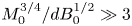 $M_0^{3/4}/ d B_0^{1/2} \gg 3$, where $M_0$ is the source momentum flux, $B_0$ is the source buoyancy flux and $d$ is the source diameter (Kaye & Hunt Reference Kaye and Hunt2006). In this regime, if the source fluid has negative buoyancy with magnitude $B$, a fountain will tend to decelerate under the buoyancy and the steady-state rise height, $Z_c$ is given by Turner (Reference Turner1966)
 \begin{equation} Z_c = 1.85 M_0^{3/4} B^{{-}1/2}. \end{equation}
The dashed line in figure 1 illustrates the rise of a turbulent fountain decelerating owing to negative buoyancy. Mingotti & Woods (Reference Mingotti and Woods2016) showed that in a uniform environment, a particle-laden fountain behaves as a classical single-phase fountain provided that the fall speed of the particles is smaller than the characteristic fountain speed. For larger particle fall speeds, the particles separate from the ascending fountain and sediment to the floor, while the particle free liquid continues upwards as a pure momentum jet.

Figure 1. Schematic plot illustrating the flow dynamics for different values of  $\sigma$.
In the context of deep submarine volcanic eruptions, the ambient stratification may have an impact on the dynamics of such fountains, and hence the fate of the particles. The dynamics of single-phase fountains rising through a stratified ambient has been studied in detail both experimentally and theoretically (Bloomfield & Kerr Reference Bloomfield and Kerr1998, Reference Bloomfield and Kerr2000; Mehaddi, Vauquelin & Candelier Reference Mehaddi, Vauquelin and Candelier2012). Through a series of experiments Bloomfield & Kerr (Reference Bloomfield and Kerr1998) demonstrated that a neutrally buoyant, momentum-driven fountain issuing from a point source, rises to an initial maximum height  $Z_m$ and then falls back to a quasi-steady-state height $Z_t \approx 0.9 Z_m$, while the collapsing fountain fluid forms a radially spreading intrusion at a height of approximately $0.5 Z_t$. Turbulent fountains in this regime are represented by the solid line in figure 1. By dimensional analysis, $Z_t$ depends on the source momentum flux, $M_0$, and the Brunt–Väisälä buoyancy frequency of the ambient fluid, $N$, according to the relation
 \begin{equation} Z_t = 3.0 \pm 0.23 M_0^{1/4} N^{{-}1/2}, \end{equation}
where the constant of proportionality was determined empirically (Bloomfield & Kerr Reference Bloomfield and Kerr1998). In the event that a negatively buoyant fountain rises through a stratified ambient, the height of rise is limited by both the source buoyancy flux and the stratification such that to good approximation
 \begin{equation} Z = min(Z_c, Z_t). \end{equation}
To distinguish the relative importance of the source buoyancy, Bloomfield & Kerr (Reference Bloomfield and Kerr1998) introduced the dimensionless parameter  $\sigma$ and found there is a smooth transition from one regime to another in the vicinity of the region
 \begin{equation} \left(\frac{Z_c}{Z_t}\right)^2 \sim \sigma^{1/2} = \frac{M_0N}{B_0} = 1, \end{equation}
where  $B_0$ is the magnitude of the buoyancy of the source flow. As mentioned above, the dynamics of particle-laden fountains in unstratified environments, corresponding to $\sigma < 1$, has been described by Mingotti & Woods (Reference Mingotti and Woods2016). In this work we complement that study, by exploring the dynamics of momentum-driven fountains in a stratified ambient, corresponding to $\sigma > 1$. In this limit, the effect of the source buoyancy is secondary, and the dominant dynamics emerges from consideration of a neutrally buoyant momentum-driven jet issuing into a stratified ambient (figure 1). The flow emerges from the source as a momentum-driven jet, however, as the fluid rises through the stratified ambient it becomes negatively buoyant owing to the decrease in the density of the environment. The direction of the buoyancy force opposes the vertical component of the momentum flux therefore the flow behaves as a turbulent fountain. The maximum height of rise of the fountains considered herein are much larger than the source radii, therefore the dynamics of these flows is analogous to high Froude number, forced turbulent fountains.
In this paper, we first present a series of laboratory experiments to describe the flow of mono-disperse particle fountains as the ratio  $U$ of the particle fall speed $V_s$ relative to the characteristic fountain speed varies. The dimensionless variable $U$ is defined as
 \begin{equation} U = \frac{V_s}{(M_0N^2)^{1/4}}. \end{equation}
In § 2, we describe the experimental techniques used. In § 3 we describe the qualitative observations from these experiments and identify two regimes, when  $U<0.1$ and $U>0.1$, in which the dynamics of the particle fountains differs significantly. When $U<0.1$, (regime I) the particles initially remain well mixed in the fountain fluid and the fountain displays behaviour analogous to single-phase fountains. We observe that in the region of $U\sim 0.1$, there is a smooth transition to a flow dynamics that is dominated by the separation of the particles in the fountain. When $U>0.1$ (regime II), the particles separate from the fluid during the initial ascent of the fountain, changing the structure of the flow. In § 4, we present some quantitative results for particle fountains as a function of the ratio $U$ and for different particle loads. In §§ 5 and 6, we compare the quantitative results of both regimes with two integral models of fountain flow following the work of Bloomfield & Kerr (Reference Bloomfield and Kerr2000) and Lippert & Woods (Reference Lippert and Woods2018). In § 7, we briefly investigate the dynamics of poly-disperse particle fountains by analysing a series of experiments in which a mixture of particles with two distinct sizes are injected into a stratified environment. We apply the theory developed in this paper to show how the regimes observed in these more complex experiments may be interpreted. Finally, we consider the implications of our work for submarine volcanic eruptions.
2. Experimental set-up
We performed a series of experiments in a Perspex tank with an internal cross-section of  $50\ \textrm {cm} \times 50\ \textrm {cm}$ (figure 2). The tank was filled to a depth of 40 cm with an aqueous saline solution using the double bucket method (Oster Reference Oster1965) to obtain a linear density stratification. The stratification of the ambient was determined before each experiment using a refractometer (Atago Palette PR-32 $\alpha$ digital refractometer, accuracy of $\pm$0.1) and the Brunt–Väisälä frequency, $N$ (s $^{-1}$), was maintained approximately constant. The variation in the temperature of the fluid was less than 5 $^{\circ }$C between experiments and the density contrast associated with this temperature range is of order $10^{-3}$. In contrast, the variation in the density associated with changing either the salt concentration or the particle mass fraction of the fluid is order $10^{-2}$. Therefore, we conclude the variation in temperature between experiments does not have a significant impact on our density measurements. It is also important to note that in all experiments the particles are dilute with concentration smaller than 0.1 and therefore we assume that there is no impact of hindered settling and that the bulk viscosity of the fountain fluid is similar to the viscosity of the ambient fluid.

Figure 2. Schematic of experimental set-up.
During an experiment, the Perspex tank was back lit using an electronic light sheet (W&Co) to ensure uniform illumination. The experiments were recorded using a Nikon D5300 digital camera with a frame rate of 50 Hz to provide sufficient time resolution, a typical experiment lasted approximately 2 min. A list of all the experiments carried out is given in table 1.
Table 1. Experimental parameters for particle fountains in a stratified environment;  $M_0$ (m $^4$ s $^{-2}$) is the source momentum flux, $Re_0$ is the source Reynolds number, $N$ (s $^{-1}$) is the Brunt–Väisälä buoyancy frequency, $Z_t/r_0$ is the fountain steady-state top height over the source radius, $C_0$ is the initial concentration of particles in the fountain mixture, $\phi$ is the volume fraction of large particles with $U>0.1$ in poly-disperse particle fountains, $B_p$ (m $^4$ s $^{-3}$) is the source buoyancy flux associated with the particle load, $D_p$ (m) is the particle diameter, $V_s$ (ms $^{-1}$) is the particle sedimentation speed, $(M_0N^{2})^{1/4}$ (ms $^{-1}$) is the characteristic fountain velocity, $U$ is the dimensionless particle fall speed.

To generate the particle-laden fountains we injected a mixture of silicon carbide particles (Washington Mills) and fresh water through a round nozzle of radius,  $r_0 = 2.5$ mm, located at the bottom of the tank. The mixture was pumped into the tank using a Watson Marlow peristaltic pump at constant volume flux, $Q_0$ (m $^3$ s $^{-1}$), and was continuously stirred throughout the experiment to maintain a constant particle flux. In this paper we present 3 sets of experiments. In the first set (experiments 1–18) the particle diameter was varied between each experiment within the range 12.8–212 $\mathrm {\mu }$m. By changing the particle diameter the sedimentation speed $V_s$ and therefore the key parameter $U$ was varied for each experiment. The sedimentation speed of the particles is given by
 \begin{equation} V_s = \frac{2}{9} \frac{\rho_p - \rho_w}{\mu_w} g \left(\frac{D_p}{2}\right)^2, \end{equation}
where  $\rho _p=3210$ kg m $^{-3}$ is the density of the particles, $\rho _w$ is the density of water, $\mu _w$ is the dynamic viscosity of water, g is the acceleration of gravity and $D_p$ is the average diameter of the particles. Each experiment was run with the addition of red dye to highlight the movement of the fluid and was repeated without the dye to image the motion of particles. In the second set of experiments (experiments (a-i)) the initial particle concentration in the source fluid was varied in the range $C_0=9\text {--}34\times 10^{-3}$ for particles with two values of $U$. In the final set of experiments (experiments I–V) we investigated the dynamics of poly-disperse particle fountains by including a combination of two distinct particle sizes in the initial source mixture, one of which remained mixed in the fountain fluid ( $U<0.1$) and one which separated during the initial rise of the fountain ( $U>0.1$). We varied the fraction of particles $\phi$ between each experiment.
In all experiments, the bulk density of the source mixture was equal to the ambient density at the base of the tank. The buoyancy flux associated with the fresh water,  $B_w$ (m $^4$ s $^{-3}$), is given by
 \begin{equation} B_w = \frac{\rho_{a,base} - \rho_w}{\rho_{a,base}} g Q_0, \end{equation}
where  $\rho _{a,base}$ is the density of the ambient at the base of the tank and the buoyancy flux associated with the particle load, $B_p$ (m $^4$ s $^{-3}$), given by
 \begin{equation} B_p = C_0 \frac{\rho_{a,base}- \rho_p}{\rho_{a,base}}\ g Q_0, \end{equation}
where  $C_0$ is the initial concentration of particles in the mixture. In all our experiments $B_w=-B_p$.
3. Qualitative observations
For reference, figure 3 is a schematic diagram illustrating the variables describing the particle fountains used herein. Figure 4(a) displays four images showing the evolution of a single-phase salt fountain in a linearly stratified ambient with zero buoyancy flux at the source (experiment (i), table 1). The salt fountain, injected upwards from the base of the tank, entrains ambient fluid whilst ascending and reaches an initial maximum height,  $Z_m$. The fluid then collapses causing a reduction in the top height of the fountain to a quasi-steady-state height $Z_t \approx 0.9 Z_m$. The fluid continues to fall until reaching a level of neutral buoyancy where it forms an intrusion which spreads radially from the fountain at a height of approximately 0.5 $Z_t$. (Bloomfield & Kerr Reference Bloomfield and Kerr1998).

Figure 3. Schematic diagram showing the variables used to described particle fountains. Regime I:  $Z_m$ is the initial fountain height, $Z_t$ is the steady-state fountain height, $Z_i$ is the initial particle-laden intrusion height, $Z_f$ is the single-phase fluid intrusion height and $R_c$ is the radius of the particle column. Regime II: $Z_p$ is the height at which the particles separate, $Z_{pt}$ is the top height of the fountain fluid.

Figure 4. (a) Series of snapshots showing the evolution of a single-phase fountain over time. (b–d) Series of snapshots from a selection of experiments showing the evolution of particle-laden fountains over time. The particles are coloured black and the source fluid is dyed red. Images show the formation of the initial intrusion  $Z_i$ and fluid intrusion $Z_f$. (e,f) Schematic diagrams showing the dynamics of particle fountains when $U<0.1$ and $U>0.1$ respectively.
Figure 4(b) displays a multi-phase fountain with black particles and the source fluid dyed red (experiment 13, table 1). In this experiment  $U = 0.045$ and so the particles remain coupled to the source fluid as the fountain ascends. As with a single-phase fountain, the initial fountain reaches a height $Z_m$ and then falls back to a near steady-state height, $Z_t$. The particle–fluid mixture at the top of the fountain is dense and falls back to form an initial intrusion at a height $Z_i\approx 0.5 Z_t$ analogous to a single-phase fountain. As the intrusion extends radially the particles fall to the base of the tank. The bulk density of the intruding fluid is reduced and it rises to a new level of neutral buoyancy $Z_f$ where a single-phase fluid intrusion is formed. Some of the particles are carried up from the original intrusion with the fluid, leading to the formation of a cloud of particles which spread radially. As these particles gradually sediment to the floor, they form a particle-laden zone with a near steady-state radius. The schematic diagram in figure 4(e) highlights the observed dynamics for particle fountains in regime I.
Figure 4(c) illustrates the case in which  $U = 0.14$ (experiment 9, table 1). In this instance the particles rise to the top of the fountain, but then separate from the down-flowing fluid whilst the flow has a radius comparable to the fountain; the initial fluid–particle intrusion at a depth $Z_i$, which was visible with a smaller value of $U$ (figure 4b), is less clear in this transitional regime. However, as before, a fluid intrusion gradually forms above the fountain, with a column of particles sedimenting below this intrusion. This experiment highlights the transitional behaviour that is observed in the vicinity of $U\sim 0.1$.
Figure 4(d) presents the case where  $U = 0.37$ (experiment 5, table 1) and the particles separate from the fountain fluid during the initial ascent of the fountain at a height $Z_p$. The fountain fluid is buoyant and rises above the particle-laden fountain top and reaches a maximum height $Z_{pt}$. The fluid then forms a single-phase intrusion upon reaching its neutral buoyancy height $Z_f$. In this case, a small volume of fountain fluid is carried downward with the particles which sediment to the base of the tank and this can be seen in the final frame (figure 4(d.iv)). The schematic diagram in figure 4(f) demonstrates the dynamics observed in regime II.
In order to help interpret the time evolution of these flows we present a selection of time series in figures (5 and 6) for fountains corresponding to four values of  $U$ (0.045, 0.095, 0.19 and 0.37), as indicated in the top row of photographs. In figure 5, the time series of vertical lines near the edge of the particle-laden zone for each fountain reveals a series of descending pulses of particles settling from just below the upper part of the fountain. In this image we have drawn a series of inclined lines which correspond to the fall speed of the particles, and it is seen that the descending particles fall with speed similar to their sedimentation speed. For the two cases, $U<0.1$, the dashed yellow lines correspond to the initial height of the particle–fluid intrusion $Z_i$. It is seen that with time, some of the fluid rises from this intrusion to a greater height where the final fluid intrusion forms, as mentioned earlier. This upward motion is indicated by the dashed upward pointing yellow arrow. The regular high frequency concentration waves observed in the vertical time series for $U >0.1$ can be attributed to the separation and sedimentation of particles in the fountain as described by Mingotti & Woods (Reference Mingotti and Woods2016). Figure 5(e) displays the settling speed of the particles as measured from the vertical time series using a Hough transform (Appendix) in comparison to the theoretical speed obtained from (2.1).

Figure 5. Letters (a–d) represent 4 different experiments with varying values of  $U$. (i) Snapshots of particle fountain at steady state. (ii) Vertical time series taken at edge of particle column (dashed vertical line in (i). The yellow solid arrow indicates particle motion at particle sedimentation speed $V_s$, yellow dashed arrow represents upward motion of fluid. (e) Particle sedimentation speed measured from descending fronts in vertical time series using a Hough transform (Appendix) in comparison to the settling speed calculated from (2.1).

Figure 6. Letters (a–d) represent 4 different experiments with varying values of  $U$. (i) Snapshots of particle fountain at steady-state. Dashed lines indicate locations of horizontal time series. (ii) Horizontal time series taken at height of initial intrusion (dot-dashed horizontal line in panel (i). The red dashed line indicates steady-state radius of particle cloud $R_c$. (iii) Horizontal time series taken at height of fluid intrusion (dashed horizontal line in panel (i)). Both time series represent 120 s.
Figure 6 shows time series of two horizontal lines for the same fountains displayed in figure 5. The first time series (ii) corresponds to the lower horizontal dot-dashed lines indicated on the snapshots (i). These time series indicate that, for small values of  $U$, there is a particle-laden zone which spreads to a nearly constant radius, $R_c$. However, as $U$ increases beyond 0.1, the radius of the particle column appears to be limited by the fountain radius, consistent with the sedimentation of particles from the fountain rather than the intrusion. The lower time series (iii) is taken from the top dashed lines indicated on the snapshots (i). These images show that the particle-free fountain fluid continues to spread radially in time above the settling column of particles. The fluid intrusion appears red on the images and so we infer that most particles have already settled from the flow. This picture of the spreading fluid intrusion is similar for all values of $U$.
$U$.
4. Quantitative observations
In addition to these qualitative observations of mono-disperse particle-laden fountains, we have measured the height of rise of the steady particle-laden fountain, the initial intrusion height of the particle-laden fluid in the case  $U<0.1$, and the ultimate intrusion height of the particle-free fountain fluid. These data are shown in figure 7(a,b) as a function of $U$ the ratio of the fall speed to the characteristic fountain speed. In this figure $\tilde {Z}$ represents the heights normalised relative to the steady-state top height of a single-phase fountain ((1.2)) with the same initial momentum flux.

Figure 7. (a) Steady-state rise height of a particle fountain  $Z_{t}$ (regime I), steady-state height of particle separation $Z_p$ (regime II) and the maximum fluid height $Z_{pt}$ as a function of $U$. (b) Height of particle-laden initial intrusion $Z_i$ and particle-free fluid intrusion $Z_f$ as a function of $U$. (c) Fluid intrusion height $Z_f$ for varying values of initial particle concentration $C_0$ where $U = 0.040$ (open circles) and $U = 0.39$ (open triangles). Dashed and dot-dashed lines indicate estimates from models used for regimes I (§ 5.1) and II (§ 5.2), respectively. All heights ( $\tilde {Z}$) are normalised relative to the steady-state top height of a single-phase fountain (cf. equation (1.2)) with the same initial momentum flux.
Figure 7(a) shows the steady-state height of rise of the particle-laden fountains for a range of  $U$. In regime I when $U < 0.1$ the steady-state height of rise is equivalent to that of a single-phase fountain with the same initial momentum flux, given by (1.2). There is a gradual decrease in the height of rise of the particle-laden fountains, as $U$ increases beyond 0.1 owing to the settling of the larger particles from the fluid. The top height of the fountain fluctuates around a steady-state value for all values of $U$ (Mingotti & Woods Reference Mingotti and Woods2016). In regime II, the maximum height of the fluid in the fountain $Z_{pt}$, which is higher than the particle separation height, increases as $U$ increases above 0.1.
Figure 7(b) shows the height of the intrusions formed as a function of  $U$. In regime I, the height of the particle-laden initial intrusion has a value $(0.5\pm 0.05)Z_t$, consistent with the fluid intrusion formed by single-phase fountains (Bloomfield & Kerr Reference Bloomfield and Kerr1998). There is no initial intrusion formed when $U >0.1$ due to the separation of particles during the initial rise of the fountain, which results in the continual ascent of the particle-depleted fountain fluid to greater heights. The height of the single-phase fluid intrusion gradually increases as $U$ increases beyond 0.1. In regime I the particle-laden fluid collapses, forms an annulus around the upflowing region and intrudes into the environment. This downflow and the subsequent particle separation entrains fluid from the ambient environment which reduces the buoyancy of the fountain fluid and in turn suppresses the ultimate height of the fluid intrusion. However, as $U$ increases, the entrainment of ambient fluid only occurs during the ascent of the fountain and this reduces the mass of dense ambient fluid in the fountain, and hence increases the fluid intrusion height.
In figure 7(c) we present data showing the height of the fluid intrusion as a function of the initial particle concentration of the source fluid which generates the fountain for the cases U=0.39 and 0.040. It is seen that the height of the fluid intrusion increases with the initial particle concentration of the fountain. Since the initial mixture of particles and fountain fluid has a bulk density which matches that at the depth of the supply nozzle in the experimental tank, the initial fountain fluid is buoyant to compensate for the excess density of the particles. Increasing the initial particle load increases this initial fluid buoyancy and therefore the height at which the fluid will intrude in the environment.
It is also of interest to note that by analysing a time series of a vertical line through the centre of the fountain, we can estimate the speed of the flow in the fountain using a Hough transform (Appendix). The speed of the flow has an approximate value
 \begin{equation} u_f=(0.13\pm0.03)(M_0N^2)^{1/4}, \end{equation}
for the range of experiments reported in this work. This is consistent with our observation of the transition in flow regimes when  $U\sim 0.1$, such that for larger fall speeds, particles begin to sediment below the top of the fountain.
5. Modelling particle fountains
As described in §§ 3 and 4, the dimensionless fall speed of the particles  $U$, has an important control on (a) the steady-state rise height of the fountain, $Z_t$; (b) whether an intrusion of particle-laden fluid, of height $Z_i$, develops; and (c) the final intrusion height of the particle-free fluid $Z_f$. To help rationalise the qualitative trends we have observed we appeal to the work of Bloomfield & Kerr (Reference Bloomfield and Kerr2000) on single-phase turbulent fountains to model the case of small particles ( $U<0.1$) for which the particles remain in the fountain until spreading out in the initial particle–fluid intrusion. As with the experiments reported by Mingotti & Woods (Reference Mingotti and Woods2016), in this limit we do not expect the particle fall speed to have a significant effect on the fountain dynamics. However, with larger $U$, the fall speed does become important in the fountain, and so we adapt the work of Lippert & Woods (Reference Lippert and Woods2018) who modelled the dynamics of turbulent bubble fountains in which bubble slip was important, to describe fountains with larger particles which fallout during their ascent in the fountain ( $U>0.1$).
5.1. Regime I:  $U<0.1$

Bloomfield & Kerr (Reference Bloomfield and Kerr2000) developed a theoretical model of single-phase turbulent fountains based on the work of Mcdougall (Reference Mcdougall1981) by describing the entrainment into the fountain on the initial upflow and the subsequent collapse. Using this model the authors were able to provide reasonable estimates of bulk parameters of single-phase fountains, such as the steady-state rise height  $Z_t$ and the initial intrusion height $Z_i$. Considering the similarities between the observations of single-phase fountains and particle fountains when $U<0.1$, we compare the predictions of this model with the present experimental data for $U<0.1$.
To account for the entrainment into the fountain, Bloomfield & Kerr (Reference Bloomfield and Kerr2000) separate the flow into two co-flowing regions and since the present experiments include both salt and particles, we account for both of these in the present development of the model. The rising inner region has radius  $r_u$, speed $u_u$, particle load $c_u$ and salinity $s_u$ and the downward collapsing outer region has outer radius $r_d$, downflow speed $u_d$, particle load $c_d$ and salt concentration $s_d$. We now describe the conservation of volume, momentum, particles and salt in both the upflow and the downflow (figure 8). The buoyancy in the upflow and downflow is defined relative to the ambient fluid
 \begin{equation} \left. \begin{array}{c@{}} g'_u = (g/\rho_0)(\rho_a(z) - \rho_0(1 + \alpha_s(s_a(z)-s_u) + \beta_p c_u)) \\ g'_d = (g/\rho_0)(\rho_a(z) - \rho_0(1 + \alpha_s(s_a(z)-s_d) + \beta_p c_d)) \end{array}\right\}, \end{equation}
where  $\rho _a(z) = \rho _0(1 + \alpha _s(s_a(z)-s(z_0))$ is the ambient density at height z above the source, $s_a(z)$ is the ambient salt concentration at height $z$,
$z$,  $\rho _0$ is the ambient density at $z=0$, $\alpha _s$ is the solutal expansion coefficient and $\beta _p = (\rho _p-\rho _0) / \rho _0$. For conservation of volume flux, we write
 \begin{gather} \frac{\textrm{d}}{\textrm{d}z}(r_u^2 u_u) = 2 r_u (\alpha u_u - \beta u_d), \end{gather}
 \begin{gather}\frac{\textrm{d}}{\textrm{d}z}([r_d^2-r_u^2]u_d) = 2 r_u (\beta u_d - \alpha u_u) + 2 r_d \beta u_d, \end{gather}
where we assume there is entrainment in both directions across the interfaces, with the entrainment coefficient for the upflow being  $\alpha = 0.085$ and for the downflow being $\beta = 0.147$. Further details of this model are given by Bloomfield & Kerr (Reference Bloomfield and Kerr2000), who demonstrated these values for the entrainment coefficients provide a good description of a salt fountain. The equations for conservation of salt (and particles), denoted by $s_u$( $c_u$) or $s_d$( $c_d$), in the upflow and downflow are
 \begin{gather} \frac{\textrm{d}}{\textrm{d}z}(r_u^2 u_u s_u) = 2 r_u (\alpha u_u s_d - \beta u_d s_u), \end{gather}
 \begin{gather}\frac{\textrm{d}}{\textrm{d}z}([r_d^2-r_u^2] u_d s_d) = 2 r_u (\beta u_d s_u - \alpha u_u s_d) + 2 r_d \beta u_d s_a, \end{gather}
where  $s_a$ ( $c_a$) is the ambient salt (particle) concentration. For the salt $s_a(z) = G_s(H-z)$ with the experimental tank being in the region $0 < z < H$, while for particles, $c_a=0$. The momentum conservation equations are given by
 \begin{gather} \frac{\textrm{d}}{\textrm{d}z}(r_u^2 u_u^2) = r_u^2 g_u' + 2 r_u \alpha u_u u_d - 2 r_u \beta u_u u_d, \end{gather}
 \begin{gather}\frac{\textrm{d}}{\textrm{d}z}([r_d^2-r_u^2] u_d^2) = [r_d^2 - r_u^2] g'_d - 2 r_u \alpha u_u u_d + 2 r_u \beta u_u u_d, \end{gather}
where  $z$ increases upwards, and $u_u>0$ while $u_d<0$. The different terms on the right-hand side correspond to the buoyancy force and the momentum loss or gain with the entrained fluid. The top height of the fountain is determined as the point where $u_u=0$. The equations are solved iteratively, integrating the equations for the upflow fountain upwards, then the downflow collapsing fluid equations are solved from the fountain top downwards to the point where $u_d=0$. The integration is then repeated until the solution converges to a steady state. An estimate of the initial intrusion height $Z_i$ can be determined by calculating the neutral buoyancy height of the downflow fluid at the point where $u_d=0$ and assuming that no further entrainment occurs into this fluid as it intrudes into the environment. Bloomfield & Kerr (Reference Bloomfield and Kerr2000) find that the estimates of the steady-state height $Z_t$ and initial intrusion height $Z_i$ from this model show good agreement with the experimental measurements of single-phase turbulent fountains in a stratified environment. We compare the numerical results of $Z_t$ and $Z_i$ using the average value of the experimental stratification and constant initial conditions as given in table 1, with our experimental measurements for $U <0.1$ in figure 7(a,b). Given the simplicity of the model, we find reasonable agreement between the numerical estimates and the experimental measurements.

Figure 8. Schematic diagram showing the implementation of the numerical models and variables used in regimes I and II. Curved solid arrows indicate that no further entrainment is accounted for and the neutral buoyancy height of the fluid is estimated from the density of the fluid. Dotted arrows indicate particle separation.
As the fluid intrudes into the environment particle sedimentation becomes progressively more important and the buoyancy of the intruding particle-free fountain fluid gradually increases. In order to estimate the height of this ultimate particle-free fluid intrusion  $Z_f$, we note that if all the particles sediment from the fluid in the particle–fluid intrusion, then the net buoyancy increases by an amount which in steady state is given by $g_p' Q_0/Q_i$ where $g_p$ is the initial particle load at the source, and $Q_i$ is the volume flux supplied to the particle–fluid intrusion. From our numerical calculations the volume flux $Q_i$ is
 \begin{equation} Q_i = 0.88 M_0 ^ {3/4} N ^ {{-}1/4}. \end{equation}
This change in buoyancy corresponds to a change in height from the original particle–fluid intrusion height  $Z_i$ to the ultimate fluid intrusion height $Z_f$ given by
 \begin{equation} Z_f = Z_i + g'_p \frac{Q_0/Q_i}{N^2}. \end{equation}
We compare the experimental measurements of  $Z_f$ with expression (5.6) in figure 7(b) where we find reasonable agreement. It is of interest to note that if we only consider the entrainment of ambient fluid into the fountain on the initial ascent and ignore the entrainment as the fluid collapses around the fountain then the fluid intrusion height is over-estimated by $\sim$10 %. By comparing the numerical estimate of the volume flux at the top of the fountain after the initial rise with the numerical estimate of volume flux in the particle-laden fluid intrusion formed from the collapsing fountain, we find an increase of approximately 40 %. This entrainment therefore has a material impact on the final height of the fluid intrusion.
5.2. Regime II: $U>0.1$

In particle fountains when  $U>0.1$ we observe the particles separate from the flow during the initial rise of the fountain. The particles sediment to the base of the tank whilst the buoyant fountain fluid continues to rise to a maximum height and then forms a single-phase intrusion. To model the dynamics in this regime we propose an upflow model for a single-phase turbulent fountain which includes the effect of the particle slip, analogous to the work of Lippert & Woods (Reference Lippert and Woods2018), who explored the dynamics of downward propagating bubble-laden fountains. We denote the horizontally averaged velocity, salt and particle concentration to be $u_u$, $s_u$ and $c_u$, while we denote the fountain radius as $r_u$ (cf. § 5.1). We introduce the variables $Q_w(z)={\rm \pi} q_w(z)$ and $Q_p(z)={\rm \pi} q_p(z)$ to represent the fluid and particle volume fluxes respectively and $M_w(z)={\rm \pi} m_w(z)$ and $M_p(z)={\rm \pi} m_p(z)$ to represent the fluid and particle momentum fluxes respectively, according to the relations
 \begin{equation} \left.\begin{array}{c@{}} q_w = r_u^2 u_u (1-c_u) , \quad q_p = r_u^2 (u_u - V_s) c_u \\ m_w = r_u^2 u_u^2 (1-c_u) , \quad m_p = r_u^2 (u_u - V_s)^2 c_u (\rho_p/\rho_0) \end{array}\right\}. \end{equation}
The entrainment of fluid into the fountain increases the volume flux (Turner Reference Turner1973; Lippert & Woods Reference Lippert and Woods2018)
 \begin{equation} \frac{\textrm{d}}{\textrm{d}z}(q_w) = 2 r_u \alpha u_u \sqrt{1-c_u}. \end{equation}
The momentum conservation is given by
 \begin{equation} \frac{\textrm{d}}{\textrm{d}z}(m_w + m_p) = r_u^2 g_u', \end{equation}
where  $g_u'$ is now given by
 \begin{equation} g'_u = (g/\rho_0)(\rho_a(z) - \rho_0(1 + \alpha_s(s_a(z)-s_u)(1-c_u) + \beta_p c_u)). \end{equation}
In the region below the sedimentation height, the particle flux is constant and the conservation of salt is given by
 \begin{equation} \frac{\textrm{d}}{\textrm{d}z}(q_p) = 0, \quad \frac{\textrm{d}}{\textrm{d}z}(q_w s_u) = 2 r_u \alpha u_u s_a(z)\quad \sqrt{1-c_u}, \end{equation}
where we adopt the entrainment coefficient for a fountain (Bloomfield & Kerr Reference Bloomfield and Kerr1998). These equations were integrated to the height at which the fluid velocity becomes equal to the particle sedimentation speed  $u_u(z) = V_s$. We define this to be the particle separation height $Z_p$. In figure 7(a) we compare the numerical prediction for the particle separation height $Z_p$ based on the average ambient stratification and the initial particle concentration for the experiments (table 1) with the experimental measurements. Data are given for a range of values of $U$. The model captures the reduction in the maximum height to which the particles are carried by the fountain as $U$ increases.
Once the particles have separated from the flow, we can model the continuing ascent of the buoyant fluid using the model for a turbulent plume (Morton, Taylor & Turner Reference Morton, Taylor and Turner1956) which is equivalent to (5.8), except there are no particles,  $c_u=0$, and the entrainment coefficient now adjusts to value $\alpha _p = 0.11$
 \begin{equation} \frac{\textrm{d}}{\textrm{d}z}(r_u^2 u_u) = 2 r_u \alpha_p u_u , \quad \ \frac{\textrm{d}}{\textrm{d}z}(r_u^2 u_u^2) = r_u^2 g_u', \quad \frac{\textrm{d}}{\textrm{d}z}(r_u^2 u_u s_u) = 2 r_u \alpha_p u_u s_a(z), \end{equation}
where  $z$ is height above the particle separation height $Z_p$. These equations were integrated until the upward momentum of the fluid was equal to zero which we define to be the maximum top height of the fluid $Z_{pt}$. Assuming that no further entrainment occurs we then estimate the height where the fluid would intrude in the ambient environment to equal the neutral buoyancy height of this plume fluid, $Z_f$. The predictions for the maximum height and the intrusion height of the fluid are shown in figure 7(a,b) and compared with the experimental data. The model provides a reasonable estimate for the fluid intrusion height for $U>0.1$ although the prediction of the maximum height suggests a greater increase in height as $U$ increases than is seen in the experiments. This may be a result of some of the momentum in the upflow being dissipated as the particles fallout, an effect not included in the model.
In the lowest part of the fountain, before the buoyancy forces become significant, we expect that the speed of the fountain may be approximated by the speed of a momentum jet
 \begin{equation} u_f \approx M_0^{1/2}/ 2\alpha z, \end{equation}
for  $z\ll Z_t$, where $Z_t = 3 M_0^{1/4}N^{-1/2}$ is the height of the equivalent fountain with $U\ll 0.1$, for which the fountain height is determined by the stratification. This approximate solution (blue dashed line) is compared with the full numerical solutions of the model ((5.7) and (5.8)) for a range of values of $U$ (solid lines) in figure 9(a). For convenience, we present the dimensionless fountain speed, defined as $u_f (2\alpha Z_t / M_0^{1/2})$, as a function of dimensionless height, $z/Z_t$, up to the point where $u_f = V_s$. In the case of large $U$, where the particles fallout well below the height at which the fountain would be arrested by the stratification, the approximation for the fountain speed ((5.10)) suggests the particle separation height scales as $Z_p = M_0^{1/2} / 2\alpha V_s$ and this scaling is in reasonable accord with the predictions of the full model for sufficiently large $U$ (figure 9b). We also note, that for $U<0.1$, the model predicts that the particle ascent in the fountain height becomes limited by the stratification. In this limit, the fountain dynamics is not dependent on the particle fall speed, and we revert to the model proposed in § 5.1.


6. Particle cloud
As the particles separate from the source fluid of the fountain, a cloud of descending particles is formed with a characteristic radius. Figure 10 shows how the time-averaged steady-state dimensionless radius of the particle cloud  $R_c / M_0^{1/4}N^{-1/2}$ varies with the dimensionless particle settling speed $U$. To provide an estimate of the radius of the column of descending particles we will consider the two regimes, $U<0.1$ and $U>0.1$, separately.

Figure 10. Time-averaged radius of the cloud of particles settling from the fountain at steady state. The dashed and solid lines represent the scalings for the radius as calculated in §§ 6.1 and 6.2 respectively. The dot-dashed line indicates the numerical estimates of the radius of the fountain as calculated from the model in § 5.2.
6.1. Regime I: $U<0.1$

When  $U<0.1$ the particles separate from the fountain fluid as the initial intrusion spreads radially at height $Z_i$ and a column of descending particles is formed. In steady state, we assume that the flux of particles sedimenting from the initial intrusion through the particle column of radius $R_c$ equals the flux of particles at the source
 \begin{equation} Q_0 C_0 = {\rm \pi}R_c^2 V_s C_c, \end{equation}
where  $C_c$ is the concentration and $V_s$ is the sedimentation speed of particles in the column. Due to the entrainment of ambient fluid in the fountain the particles are more dilute in the column than at the source. We can estimate the concentration of particles in the column using our numerical solution for the volume flux in the initial intrusion $Q_i$ obtained from the model described in § 5.1
 \begin{equation} C_c = C_0 \frac{Q_0}{Q_{i}}. \end{equation}
By combining (6.1) and (6.2) we find (Mingotti & Woods Reference Mingotti and Woods2019)
 \begin{equation} {\rm \pi}R_c^2 V_s = Q_{i}, \end{equation}
and substituting (5.5) into 6.3 we can express  $R_c$ as
 \begin{equation} R_c = 0.53 M_0 ^ {1/4}N^ {{-}1/2}U^ {{-}1/2}, \end{equation}
and this model is shown by the dashed line in figure 10.
6.2. Regime II: $U>0.1$

In the limit of large  $U$, figure 9 suggests that the particles separate from the fountain at the approximate height $M_0^{1/2}/(2 \alpha V_s)$. At this point, the radius of the fountain is given by $2 \alpha z$. Assuming the particles fall directly to the ground, we therefore expect the particle radius to scale with the fountain radius
 \begin{equation} R_c = \frac{M_0^{1/2}}{V_s}, \end{equation}
and this may be rewritten in the form
 \begin{equation} R_c = \frac{M_0^{1/4}N ^{{-}1/2}}{U}. \end{equation}
This relation is shown as the solid line in figure 10. In addition, we present the numerical estimate of the radius of the fountain  $r_u$ at the height $Z_p$ as calculated from the model in § 5.2 (dot-dashed line). As expected this approaches this limit ((6.6)) for large $U$. The experimental data (circles) appear to follow the trend for the small particles ( $U<0.1$, (6.4)) and appear consistent with a transition towards the dot-dashed line for $U>0.1$, but the range of values of $U$ possible in our experimental system does not allow us to fully test the limit of large $U$ ((6.6)).
7. Poly-disperse particle fountains
We have, thus far, only considered the simplified case of mono-disperse particle-laden fountains in a stratified environment. However, in a more realistic setting, naturally forming particle-laden fountains may consist of a distribution of particle sizes. To investigate the dynamics of these more complex flows we introduce the case of a particle-laden fountain with zero source buoyancy flux containing a fraction  $\phi$ of large particles that separate from the fountain on its initial ascent ( $U>0.1$) and a fraction $(1-\phi )$ of particles that stay entrained in the fluid ( $U<0.1$) (experiments I–V, table 1). For example, a fountain with $\phi = 0$ corresponds to a mono-disperse particle-laden fountain in the regime $U<0.1$.
Similar to mono-disperse particle fountains, as the fountain rises on its initial ascent through the ambient fluid there is a height  $Z_p$ at which the large particles separate from the flow and sediment to the base of the tank. The small particles with $U<0.1$ remain entrained in the source fluid. The local buoyancy of this remaining mixture is a function of the buoyancy of the source fluid, the remaining particle load and the entrained fluid and it may be positive or negative.
If  $\phi$ is small the increase in the buoyancy as the large particles separate is small and the residual particles and fluid may still be negatively buoyant and collapse, as shown in the snapshot and schematic figure 11(a). The collapsing mixture forms an initial particle–fluid intrusion at an intermediate height between the base of the tank and the fountain top. The small particles then sediment from the intrusion and the buoyant fountain fluid rises to form a single-phase fluid intrusion. The behaviour of fountains in this regime displays clear similarities to mono-disperse particle fountains when $U<0.1$.

Figure 11. Snapshot and schematic diagram highlighting the dynamics observed in poly-disperse particle fountains when (a)  $\phi =0.25$ and (b) $\phi =0.75$. (c) Buoyancy of residual particle and fluid mixture at height $Z_p$ estimated from the model described in § 5.2.
In contrast, if the fraction  $\phi$ of particles in the fountain is large, the separation of the particles may cause the remaining mixture of small particles and fluid to become positive. In this case, the mixture rises to form an initial intrusion above the height of particle separation, as shown in figure 11(b). The small particles sediment from the intrusion and a single-phase fluid intrusion forms above the initial intrusion height as a result. The dynamics observed in poly-disperse fountains in this regime can be compared to that of mono-disperse particle fountains in the regime $U>0.1$.
The initial fraction of large particles and their subsequent separation has an observable effect on the structure of these fountains. The separation of the large particles in poly-disperse fountains has some features common with the separation of particles in mono-disperse fountains with  $U>0.1$. If we apply the model developed in this paper for the ascent of mono-disperse particle fountains with $U>0.1$ (§ 5.2) we can estimate the height where the fountain velocity is equal to the sedimentation speed of the large particles. This provides an approximation for the height of particle separation. At this point we assume that the fraction of large particles $\phi$ separate from the flow and we calculate the buoyancy of the residual mixture. Given average values of the experimental conditions (experiments I–V) we have estimated the buoyancy of the residual mixture as a function of $\phi$ and the numerical results are presented in figure 11(c). The model estimates a reversal in the buoyancy of the remaining particles and fluid when $\phi \sim 0.75$, which is consistent with our qualitative observations, and suggests in general, that as $\phi$ increases there may a change in regime from (I) to (II).
However, owing to the complexity of the resulting multi-phase flows, with both small and large particles, we do not attempt to further model their dynamics in this paper. The interaction of the residual fluid with the ambient fluid and the initial ascending fountain will be the focus of future study.
8. Summary and application
We have presented an experimental study of particle-laden fountains in a stratified environment. By varying the dimensionless fall speed of the particles,  $U$, we have identified two distinct regimes with smooth transition between the two when $U\sim 0.1$. In regime I when $U<0.1$, particles are initially well coupled to the source fluid on the initial ascent of the fountain and the fountain behaves essentially as a single-phase fountain in a stratified environment. The particle-laden fluid intrudes at the height of the equivalent single-phase fountain intrusion and spreads radially. As particles settle from the intrusion, the intruding fluid rises to form a single-phase intrusion while the settling particles form a descending column. In regime II with $U>0.1$, the particles separate from the source fluid in the fountain, causing a reduction in the steady-state height of the fountain and the fountain fluid continues rising to form a fluid intrusion. By considering two separate models describing the evolution of multi-phase turbulent fountains in a stratified ambient we have been able to approximate bulk parameters of the particle-laden fountains such as the initial and fluid intrusion heights and rationalise the trends observed in these parameters as the particle size varies. We have shown that the dynamics of simple poly-disperse flows shows clear similarities with their mono-disperse counterparts, however, this requires more detailed study.
The results of the present study provide useful insight when considering explosive submarine volcanic eruptions. These involve the eruption of a mixture of fragmented ash and pumice in a turbulent gas suspension. Once the erupting material has mixed with a sufficient mass of sea water, there will be a transition to a particle-laden flow of hot water, ash and pumice, with volume flux of order (1–10)  $Q_0$, momentum flux of order 100 $Q_0$ and buoyancy flux of order (0.1–10) $Q_0$, where $Q_0$ is the initial volume flux from the vent. In deep water, with $N\approx 0.01\text {--}0.03$ s $^{-1}$, we estimate that $\sigma$ may be of order $\sim$1–10, and so the flow will have dynamics with features of the particle-laden jets considered herein. With weak ambient currents, and $Q_0$ in the range $10^3\text {--}10^5~$m $^3$ s $^{-1}$, the characteristic fountain speed is 1–5 ms $^{-1}$. This suggests that pyroclasts with fall speed $V_s > 0.1$ ms $^{-1}$ ( $D_p > 0.01$ m) tend to sediment close to the source, after falling from the fountain as in regime II above, whereas pyroclasts with fall speed $V_s < 0.1$ ms $^{-1}$ ( $D_p < 0.01$ m) tend to be carried radially outwards and have a much larger dispersal radius, equivalent to regime I above. These results are shown in figure 12, for $Q_0 = 10^3$, $10^4$ and $10^5$ m $^3$ s $^{-1}$. These general predictions are consistent with field observations (Sohn et al. Reference Sohn2008) of the deposits and in specific situations may enable a simple estimate of the eruption flux. We plan to explore this in more detail in future work.

Figure 12. Estimated radial extent from a submarine eruption fountain of pyroclasts as a function of particle diameter. Calculations correspond to the initial conditions in § 8, with the average equivalent density of pyroclasts being  $\rho _p=2500$ kg m $^{-3}$. The solid lines represent the estimate of the radius of the particle column obtained when $U<0.1$ (§ 6.1) and the dot-dashed line displays the estimate of the radius when $U>0.1$ (§ 6.1).
Declaration of interests
The authors report no conflict of interest.
Appendix. Hough transform
To measure the speed of the rising fountain and the speed of the sedimenting particles in our experiments we follow the method of Rocco & Woods (Reference Rocco and Woods2015) using a Hough transform. Figure 13(a) shows a section of a time series of a vertical lines of pixels taken at the centreline of a fountain from typical experiment. The forward-sloping lines apparent in this image represent rising parcels of particles and fluid at the core of the fountain. We are able to estimate the speed of these rising parcels by calculating the average gradient of the forward-sloping lines using the edge detection function (figure 13b) and Hough transform (figure 13c) provided in the Image Processing Toolbox by MATLAB (2018). This process was repeated for each experiment and an average value of the speed of the flow calculated. This procedure was also carried out to calculate the speed of the sedimenting particle using the time series shown in figure 5.

Figure 13. Procedure used to estimate the speed of the rising fountain flow in our experiments. (a) Grey scale centreline time series showing rising fountain mixture (forward-sloping lines), (b) output of the edge detection function in Matlab and (c) output of Hough transform used to calculate the gradient of the forward-sloping lines in the time series.


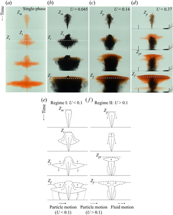


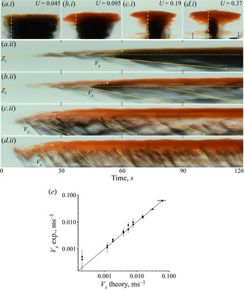


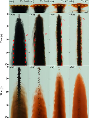


 Open access