


1. Introduction
Free-surface flows of fluids that have a yield stress are common in the environment. Examples include lava flows, fluidised mine tailings, mud slides and avalanches (Coussot & Proust Reference Coussot and Proust1996; Fink & Griffiths Reference Fink and Griffiths1998; Hu & Bürgmann Reference Hu and Bürgmann2020). Often these flows interact with topography and obstructions such as trees and constructed barriers (Tai et al. Reference Tai, Gray, Hutter and Noelle2001; Barberi et al. Reference Barberi, Brondi, Carapezza, Cavarra and Murgia2003; Dietterich et al. Reference Dietterich, Cashman, Rust and Lev2015; Bernabeu, Saramito & Harris Reference Bernabeu, Saramito and Harris2018; Chevrel et al. Reference Chevrel, Harris, Ajas, Biren, Gurioli and Calabrò2019). However, the all-important role of the yield stress that influences these interactions is not well-understood. In this paper, we analyse the steady interaction between a free-surface viscoplastic flow (with negligible inertia) and a cylindrical obstruction on an inclined plane (see figure 1a).

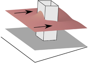
Figure 1. (a) Schematic of the steady free-surface flow. (b) Schematic of the flow along the centreline indicating the kinematically plugged region, which comes to encompass the entire layer near the stagnation points. (c) Steady flow thickness for  $B=1$ and $\mathcal {L}=1$. (d) Corresponding height of the yield surface, $Y$.
$Y$.
There has been substantial research on Newtonian free-surface flows around obstructions, which provides a foundation for analysing the viscoplastic case. Investigating these flows is challenging owing to their nonlinear governing equations, even when a lubrication approximation is applied. This has motivated a multitude of numerical methods to simulate the motion including boundary integral formulations and finite element techniques (Baxter et al. Reference Baxter, Power, Cliffe and Hibberd2009; Sellier et al. Reference Sellier, Lee, Thompson and Gaskell2009). These works focused on very thin films, in which the effects of interfacial surface tension play a key role. Some of the observed features, such as a capillary ridge upstream of a step-down in the substrate, appear only when surface tension is dominant (Kalliadasis, Bielarz & Homsy Reference Kalliadasis, Bielarz and Homsy2000). However, other results, including the horseshoe-like flow deflection, are universal to the interaction of slow flows with obstructions, even when gravity dominates surface tension.
Steady viscous free-surface flows around cylinders of various cross-sections have recently been studied by Hinton, Hogg & Huppert (Reference Hinton, Hogg and Huppert2020). They showed that the width of the cylinder relative to the thickness of the oncoming flow (and the slope inclination) was the key parameter determining the nature and magnitude of the interaction, and they constructed asymptotic solutions in both the regimes of very narrow and very wide obstructions. The latter can be encapsulated in a simple balance of volume fluxes that enables the prediction of the upstream flow thickness in the relatively deep flow just upstream of the obstruction. The key idea was that the flux in the normal direction to the obstruction vanishes throughout the upstream deep region resulting in a ‘pond’-like free-surface.
In this contribution, we focus on steady flows of viscoplastic materials, which are characterised by a ‘yield stress’. For deviatoric stresses below the yield stress, the material is rigid and when the yield stress is exceeded, the material yields and flows as a fluid albeit with an adjusted relationship between the stress and rate of strain tensor. Free-surface viscoplastic flows generally consist of two distinct regions. Near the substrate over which the material flows, there is typically a sufficiently large shear stress so that the material yields with a significant velocity gradient perpendicular to the substrate. In the upper portion of the layer the material is rigid since the stress vanishes at the free surface. The layer is partitioned into a yielded region below a rigid region with the boundary known as the ‘yield surface’. This simple description can require a subtle alteration to be compatible with lubrication theory. In cases where the thickness varies along the flow, the stress in the upper region just exceeds the yield stress with the vertical velocity gradient being negligible but non-zero (Balmforth & Craster Reference Balmforth and Craster1999). In this case, the upper region behaves kinematically as a rigid (pseudo) plug but its slight yielding allows extensional variation in the flow. It is also worth noting that when the (pseudo) plug extends down to the substrate, the entire layer is truly rigid.
Previously, obstructed viscoplastic flows have mostly been studied in the context of simplified geometries. Examples include flow in the narrow gap between two plates with an obstacle present in the conduit, known as a Hele-Shaw cell (Hewitt et al. Reference Hewitt, Daneshi, Balmforth and Martinez2016; Daneshi et al. Reference Daneshi, MacKenzie, Balmforth, Martinez and Hewitt2020), and two-dimensional flow past a cylinder (Mitsoulis Reference Mitsoulis2004; Tokpavi, Magnin & Jay Reference Tokpavi, Magnin and Jay2008). In the Hele-Shaw flow, the fluid in the far field is driven by a background pressure gradient so that it is yielded across part of the gap thickness. However, the material becomes rigid across the entire thickness in stagnant ‘dead’ zones upstream and downstream of the obstruction.
For the flow set-up considered in the present paper (figure 1a), the far-field flow must be yielded near the inclined plane whilst fully rigid, ‘dead’ zones may appear both immediately upstream and downstream of the obstruction. The steady interaction of such flows with an isolated topographic mound was studied by Hinton & Hogg (Reference Hinton and Hogg2022). They showed that the yield stress of the fluid reduces the diversion of flux around the mound and also leads to a thicker accumulation of fluid upstream of the mound. In this study we investigate the flow around a surface-piercing cylindrical obstruction, which is substantially different to flow over a mound with smoothly varying topography. However, the downstream reconnection of the flow in the lee of tall and wide mounds and obstructions is similar.
There are some analogies with obstructed free-surface granular flows despite the importance of inertia in that context. Examples include the long dead zone downstream of wide obstructions and that in the stagnant dead zone upstream, the material is on the verge of flowing (Cui & Gray Reference Cui and Gray2013; Tregaskis et al. Reference Tregaskis, Johnson, Cui and Gray2022).
The paper is structured as follows. The model is described in § 2 with the flow governed by two dimensionless groups. Numerical results for the flow thickness and the dead zones are reported in § 3, with full details of the numerical implementation given in Appendix A. In § 4, we analyse flow around relatively wide obstructions. A flux balance argument is deployed to quantify the flow thickness and this identifies the role played by the yield stress. Some of the peripheral asymptotic details are given in Appendix B. The case of relatively narrow obstructions is then investigated in § 5, where we show that there is an equivalence with flow in a Hele-Shaw cell (Hewitt et al. Reference Hewitt, Daneshi, Balmforth and Martinez2016), a connection that allows the shape of the dead zone to be approximated. Concluding remarks are given in § 6. Throughout we focus on obstructions with square cross-section but give the key differences for a rhombus-shaped cross-section in Appendix C and circular cross-section in Appendix D.
2. Theoretical model
We analyse the steady free-surface flow of a Bingham fluid on an inclined plane at angle  $\beta$ to the horizontal (figure 1a). We consider a Bingham fluid because it has the simplest constitutive law that exhibits a yield stress enabling us to identify the influence of this phenomenon. In Bingham's model, the fluid is rigid for stresses below the yield stress, $\hat {\tau }_Y$ and the fluid yields with (constant) shear viscosity $\hat {\mu }$ when the yield stress is exceeded (Bingham Reference Bingham1916; Balmforth & Craster Reference Balmforth and Craster1999). The fluid has constant density $\hat {\rho }$. The coordinate axes are oriented as follows: the $\hat {x}$ axis is directed downslope, the $\hat {y}$ axis cross-slope and the $\hat {z}$ axis is perpendicular to the plane (with $\hat {z}=0$ on the plane surface). The steady flow thickness is denoted by $\hat {h}(\hat {x},\hat {y})$. The flow is obstructed by a rigid obstruction with square cross-section lying in $(\hat {x},\hat {y}) \in [-\hat {L},\hat {L}]\times [-\hat {L},\hat {L}]$, which is assumed to be sufficiently tall that the flow never surmounts the obstruction.
The flow is supplied by a line source, with infinite extent in the  $\hat {y}$ direction, which is located far upstream of the obstruction and delivers a sustained flux $\hat {Q}_{\infty }$ per unit length. We assume that the flow is relatively thin, inertia-less and that surface tension is negligible. A lubrication approximation is applied and so no-slip is not imposed on the obstruction boundary; the effects of friction on the obstruction walls is confined to a small unimportant boundary layer that we neglect (see Balsa Reference Balsa1998). The boundary conditions are therefore no flux on the obstruction boundaries and that the flow thickness returns to its unperturbed constant value far from the obstruction, which we denote $\hat {H}_{\infty }$.
We non-dimensionalise in plane lengths with the obstruction half-width,  $\hat {L}$, and flow thicknesses with the thickness of Newtonian flow with viscosity $\hat {\mu }$ (Nusselt Reference Nusselt1916)
 \begin{equation} {\hat{H}_N = \left(\frac{3 \hat{\mu} \hat{Q}_{\infty}}{\hat{\rho} \hat{g} \sin \beta} \right)^{1/3}}. \end{equation}
This choice of thickness scale ensures that the dimensionless upstream flux is unity for any value of the yield stress. It is equivalent to scaling the flux with  $\hat {Q}_{\infty }$. The dimensionless variables are
 \begin{equation} {(x,y)=(\hat{x},\hat{y})/\hat{L}}, \quad (z,h)=(\hat{z},\hat{h})/\hat{H}_N. \end{equation}
The governing equation for the flow is derived by balancing in-plane hydrostatic pressure gradients with the divergence of shear stress. The stress vanishes at the free surface and so the material is always unyielded to leading order in a neighbourhood of the free surface (Balmforth & Craster Reference Balmforth and Craster1999). If the stress at the substrate ( $z=0$) exceeds the yield stress then the layer is partitioned into a yielded region below a pseudo-plugged region; otherwise the entire layer is rigid and stationary (see figure 1b). Then using the Bingham constitutive law, the velocity field is obtained. Integrating over the flow thickness enables the dimensionless volume flux parallel to the plane, $\boldsymbol {q}$, to be calculated in terms of the flow thickness and its gradient (see Balmforth, Craster & Sassi Reference Balmforth, Craster and Sassi2002)
 \begin{equation} \boldsymbol{q} = \frac{1}{2}Y^2(3h-Y)\left(1- \mathcal{L}^{-1} \frac{\partial h}{\partial x}, -\mathcal{L}^{-1} \frac{\partial h}{\partial y}\right), \end{equation}
where the height of the yield surface is
 \begin{equation} Y(x,y) = \max \left(0,h - \frac{B}{\sqrt{\left(1-\mathcal{L}^{-1} \dfrac{\partial h}{\partial x}\right)^2 +\left(\mathcal{L}^{-1} \dfrac{\partial h}{\partial y}\right)^2}}\right), \end{equation}
and the flow is governed by two dimensionless parameters
 \begin{equation} {B = \frac{\hat{\tau}_Y}{\hat{\rho} \hat{g} \hat{H}_N \sin \beta}, \quad \mathcal{L}=\frac{\hat{L} \tan \beta}{\hat{H}_N}.} \end{equation}
The former is the Bingham number, which is the ratio of the yield stress to a characteristic gravitationally induced stress, whilst the latter is an aspect ratio, which is associated with the relative width of the obstruction. The terms in the large brackets in (2.3) can be written as  $(1,0)-\mathcal {L}^{-1}\boldsymbol {\nabla } h$, which reveals the effect of hydrostatic pressure gradients associated with the inclined plane and the free-surface shape, respectively. The latter acts to smooth free-surface gradients. The flow is yielded in $0< z< Y$ and pseudo-plugged in $Y< z< h$. In regions where $Y=0$, the entire thickness of the layer is truly plugged (e.g. figure 1b). The steady flow satisfies
 \begin{equation} \boldsymbol{\nabla}\boldsymbol{\cdot} \boldsymbol{q} =0, \end{equation}
with  $\boldsymbol {q} \boldsymbol {\cdot }\boldsymbol {n} = 0$ on the obstruction boundaries.
Under this formulation, the dimensionless flux per unit width is unity far upstream;  $\boldsymbol {q} \to (1,0)$ as $x \to -\infty$. The dimensionless flow thickness satisfies $h\to h_{\infty }=\hat {H}_{\infty }/\hat {H}_N$ far from the obstruction with $h_{\infty }$ given by the solution to the following (far-field) flux balance
 \begin{equation} 1= (h_{\infty} - B)^2(h_{\infty} +B/2). \end{equation}
The relationship between  $h_{\infty }$ and $B$ is shown in figure 2 as a black line. For all $B$, we have $h_{\infty }>\max (1,B)$, and for small $B$,
$B$,
 \begin{equation} h_{\infty} = 1+ B/2 + \ldots, \end{equation}
whilst for large  $B$,
$B$,
 \begin{equation} h_{\infty} = B + \left(\frac{2}{3B} \right)^{1/2} + \ldots. \end{equation}
These predictions are included in figure 2 as red and blue dashed lines.


3. Numerical results and general observations
The system consisting of (2.3), (2.4) and (2.6), with boundary conditions of no-flux on the obstruction boundaries and  $h\to h_{\infty }$ as $x^2+y^2 \to \infty$ is integrated numerically to find the steady flow thickness $h(x,y)$. Full details of the numerical method are given in Appendix A. The flow thickness calculated from the numerical method for $B=1$ and $\mathcal {L}=1$ is shown in figure 1(c). The domain of the numerical computation extends far beyond the region plotted in the figures. The steady flow deepens upstream of the obstruction and thins downstream of the obstruction. Our numerical results confirmed that the streamwise extent of the obstruction has a negligible influence on the upstream and downstream flow. We focus on square obstructions noting that almost identical results apply to rectangular cross-sections with the same width.
Throughout this paper, we analyse how the flow direction and thickness is influenced by the obstruction, with particular focus on the dependencies on the relative obstruction width (via  $\mathcal {L}$) and the relative magnitude of the yield stress (via $B$). We find that the flow behaviour is delineated into four asymptotic regimes, shown in parameter space in figure 3. These regimes are partitioned into the case that the obstruction is wide relative to the flow thickness ( $\mathcal {L} \gg h_{\infty } \approx \max (1,B)$) and the case that the obstruction is relatively narrow, on the right-hand and left-hand side of parameter space, respectively. The ‘wide’ regime is analysed first in § 4 and the ‘narrow’ regime in § 5.

Figure 3. The four regimes of flow around a square obstruction in ( $\mathcal {L}$, $B$)-parameter space. The colour maps represents the steady flow thickness, $h(x,y)$. The wide regimes are shaded grey.
However, before launching into the analysis for each of these regimes, we comment on two general features of the flow; ‘dead’ zones at the stagnation points (§ 3.1), and the potential for non-unique solutions (§ 3.2).
3.1. Dead zones at the stagnation points
The height of the yield surface in figure 1(d) illustrates that ‘dead’ zones, in which the material is entirely rigid and static, develop upstream and downstream of the obstruction. Although the yield stress is regularised somewhat in our numerical scheme (see Appendix A), the log scale enables the distinction of the dead zone to be clearly seen as black regions in figure 1(d) (here we have chosen the dead zone to correspond to  $Y \lesssim 2 \times 10^{-4}$ though this arbitrary threshold has little influence on the interpretation of the flow structure).
For  $B>0$, there is always a dead zone in a neighbourhood of the two stagnation points at $(\pm 1,0)$; see, e.g., figure 4. This is easily argued by contradiction. Suppose that the material is yielded at $z=0$ at $(\pm 1,0)$ with $Y>0$. Then, by symmetry, the transverse flux $\boldsymbol {q}\boldsymbol {\cdot } \boldsymbol {e}_y$ vanishes, and by the boundary condition on the wall, $\boldsymbol {q}\boldsymbol {\cdot } \boldsymbol {e}_x$ vanishes (where $\boldsymbol {e}_x$ and $\boldsymbol {e}_y$ are unit vectors in the $x$ and $y$ directions, respectively). With $Y>0$, (2.3) furnishes $\partial h/\partial y=0$ and $\partial h/\partial x= \mathcal {L}$. The yield stress term in (2.4) is then singular implying that $Y=0$, a contradiction. The material is always rigid at these locations because the flow stagnates there and there is no hydrostatic pressure gradient to induce any shear stress in the layer.

Figure 4. (a) Steady flow thickness,  $h(x,y)$, and (b) yield surface height, $Y(x,y)$, for $B=1$ and $\mathcal {L}=4$ (calculated numerically); (c) $h(x,y)$ and (d) $Y(x,y)$ for $B=1$ and $\mathcal {L}=16$.
The size of the two dead zones increases with the dimensionless yield stress  $B$. The upstream dead zone becomes smaller for wider obstructions (greater $\mathcal {L}$) whilst the downstream dead zone becomes larger (e.g. figure 4). This is because for greater $\mathcal {L}$, the magnitude of the ‘smoothing’ term, $-\mathcal {L}^{-1} \boldsymbol {\nabla } h$ in (2.3) is diminished. Hence, the cross-slope gradient of the free surface at the upstream boundary is larger in order to divert the flow (see § 4), and the flow reconnects downstream over a greater distance (see Hinton & Hogg Reference Hinton and Hogg2022).
A simple corollary is that there can be a ‘cusp’ at the upstream stagnation point, i.e.  $\partial h/ \partial y$ is discontinuous. This is a common feature of plugged viscoplastic material (Balmforth et al. Reference Balmforth, Craster and Sassi2002). The cusp is borne out by our asymptotic analysis for relatively wide obstructions. It is slightly smoothed in the numerical results owing to the regularisation of the yield stress.
3.2. Non-uniqueness of the steady flow
Throughout this paper, we primarily focus on the upstream flow, noting that for  $\mathcal {L} \gg 1$ there is a long dead zone downstream of the obstruction and the flow will reconnect over a length scale proportional to $\mathcal {L}$ (Hinton & Hogg Reference Hinton and Hogg2022). Details of the flow structure at the edge of the downstream dead zone and the possibility of a non-unique steady state were investigated in Hinton & Hogg (Reference Hinton and Hogg2022) for flow around large mounds corresponding to $\mathcal {L} \gg 1$. The steady state downstream will depend on the initial condition prior to the supply of constant flux from upstream. For example, the plane may have been entirely dry with $h=0$ everywhere in which case the downstream dead zone mostly corresponds to a dry zone with $h=0$ (provided that $\mathcal {L} \gg 1$). If instead, the plane was coated with a uniform, rigid and stationary layer of fluid with thickness $h=B$ prior to the line source initiation, then the downstream dead zone would mostly be a region in which $h=B$. In the numerical results presented in this paper, we have assumed that this is the case; see, for example, figure 4. It should also be noted that any $0\leqslant h \leqslant B$ is allowed in the downstream dead zone provided that the layer is entirely rigid. Importantly, the downstream behaviour has negligible effect on the upstream thickness.
4. Flow past a relatively wide obstruction ( $\mathcal {L} \gg h_{\infty }$)

For a relatively wide obstruction ( $\mathcal {L} \gg h_{\infty } \approx \max (1,B)$), there is significant flow deepening at the upstream boundary; see figures 3 and 4. In addition, there is a long dead zone downstream. This regime is consistent with lubrication theory provided that
 \begin{equation} \mathcal{L} \gg \max(h_\infty, h_\infty \tan \beta). \end{equation}
Upstream of a wide obstruction, the fluid forms a deep pond. The extent of the pond in the  $x$ direction is much smaller than the width of the obstruction; e.g. figure 4(c). Hence, $\partial /\partial x \gg \partial /\partial y$ and since there is no flux into the obstruction, we have $\boldsymbol {q} \boldsymbol {\cdot } \boldsymbol {e}_x \approx 0$ over the extent of the pond, where $\boldsymbol {e}_x$ is the unit vector in the $x$ direction. This corresponds to a free surface that is horizontal in the streamwise direction (i.e. perpendicular to the direction of gravity), as has been observed previously for Newtonian flow past obstructions (Hinton et al. Reference Hinton, Hogg and Huppert2020). These observations motivate writing the flow thickness in the deep region as
 \begin{equation} h=(1+x)\mathcal{L} + G(y), \end{equation}
where  $G(y) \gg 1$ is the flow thickness on the upstream boundary, $x=-1$, which is to be determined by equating the flux arriving into the deep pond from upstream with the transverse flux along the pond. In the pond, the yield surface is located at
 \begin{equation} Y=\max\left(0, (1+x) \mathcal{L}+G(y) - \frac{B}{\mathcal{L}^{-1} |G'(y)|}\right). \end{equation}
The volume flux arriving into the pond from upstream in  $[0,y]$ is $y$ since the dimensionless flux far upstream is unity per unit length. The transverse flux at $y$ is calculated from (2.3) over the region in which $Y >0$. The steady flux balance takes the form (cf. Lister & Hinton Reference Lister and Hinton2022)
 \begin{equation} y=\int_{pond} \boldsymbol{q} \boldsymbol{\cdot} \boldsymbol{e}_y \, \mathrm{d}\kern0.7pt x= \int_{Y>0} - \textstyle{\frac{1}{2}} \mathcal{L}^{-1} Y^2 (3h-Y) G'(y)\, \mathrm{d}\kern0.7pt x. \end{equation}
We recast this as an integral over  $Y$ using (4.2) and (4.3)
 \begin{equation} y=- \mathcal{L}^{-2} G'(y) \int_0^{Y_0} Y^2\left(Y+ \frac{3B}{2 \mathcal{L}^{-1} |G'(y)|}\right) \mathrm{d} Y. \end{equation}
 Note that  $Y$ is a linearly increasing function of $x$, and
 \begin{equation} Y_0=Y(x=-1)=\max\left(0,G(y) - \frac{B}{\mathcal{L}^{-1}|G'(y)|}\right) \end{equation}
is its maximum value at the wall  $x=-1$. Carrying out the integration furnishes
 \begin{equation} y = \frac{-\mathcal{L}^{-2} G'(y)}{4} \left( G(y) - \frac{B}{\mathcal{L}^{-1} |G'(y)|}\right)^3 \left( G(y) + \frac{B}{\mathcal{L}^{-1} |G'(y)|}\right). \end{equation}
The left-hand side represents the flux from upstream and the right-hand side represents the transverse flux. Equation (4.7) is a nonlinear first-order ordinary differential equation (ODE) with boundary condition  $G(1)=0$ corresponding to the flow thickness returning to lower order at the sides of the obstruction (e.g. figure 4c). The dominant balance in this equation differs depending on the relative magnitude of $\mathcal {L}$ and $B$.
$B$.
For a Newtonian fluid ( $B=0$), (4.7) gives the pond depth as $G \sim \mathcal {L}^{2/5}$ (Hinton et al. Reference Hinton, Hogg and Huppert2020). This suggests that the relative importance of the yield stress terms in (4.7) is given by the quantity $B \mathcal {L}^{1/5}$. These observations motivate defining
 \begin{equation} \lambda = B \mathcal{L}^{1/5} \quad \text{and} \quad G(y) = \mathcal{L}^{2/5} \bar{G}(y). \end{equation}
Equation (4.7) becomes
 \begin{equation} y = \frac{-\bar{G}'}{4} \left( \bar{G} - \frac{\lambda}{ |\bar{G}'|}\right)^3 \left( \bar{G}+ \frac{\lambda}{|\bar{G}'|}\right). \end{equation}
The rescaled flow thickness at the wall,  $\bar {G}(y)$, depends only on the single parameter, $\lambda$, which represents the relative importance of the yield stress. Equation (4.9) is integrated numerically using the boundary condition $\bar {G}(1-\delta )=(20 \delta )^{1/5}$, where $\delta = 10^{-8}$. At each step in the negative $y$ direction, $\bar {G}'$ is obtained by applying Newton's method to (4.9), with the restriction that the terms in brackets are positive.
The solution for  $\bar {G}(y)=h(x=-1,y)/\mathcal {L}^{2/5}$ is shown as black lines in figure 5(a) for $\lambda =0.1$, $1$ and $10$. The magenta stars in figure 5(a) represent the thickness at the wall ( $x=-1$) from the full numerical integration of the governing partial differential equation, with $\mathcal {L}=20$ and $B$ chosen to give the required value of $\lambda$. The red dashed and blue dot-dashed lines are the small and large yield stress asymptotic results obtained in §§ 4.1 and 4.2. Figure 5(b) shows the rescaled maximum thickness (i.e. $h(-1,0)$) as a function of $\lambda$ with the lines calculated as in figure 5(a).

Figure 5. (a) Rescaled flow thickness at the wall  $x=-1$ as a function of cross-slope position. (b) Rescaled maximum flow thickness as a function of $\lambda$. The black lines are obtained by integrating (4.7). The results from the full numerical method with $\mathcal {L}=20$ are shown as magenta stars. The red dashed and blue dot-dashed lines are the small and large yield stress asymptotic predictions, respectively (see §§ 4.1 and 4.2).
The flow thickness increases for larger  $\lambda$. A steeper free surface is required to divert the upstream flux at higher yield stresses because a greater proportion of the layer is rigid. The relative importance of the plugged material in the overall flow depends primarily on $B$ but also weakly on $\mathcal {L}$; wider square obstructions exacerbate the plug size because the term in the stress associated with the transverse free-surface gradient, $-\mathcal {L}^{-1} \partial h/\partial y$ is smaller. Note that this does not occur for obstructions with walls that are angled to the downslope direction because the free-surface gradient is not the dominant contribution in the yield stress term; see Appendix C. We analyse the low and large yield stress regimes in §§ 4.1 and 4.2, respectively.
4.1. Relatively low yield stress ($\lambda \ll 1$)

In terms of the two original dimensionless groups,  $B$ and $\mathcal {L}$, the present $\lambda \ll 1$ regime is (see figure 3)
 \begin{equation} {B \ll \mathcal{L}^{-1/5}, \quad \mathcal{L} \gg 1.} \end{equation}
This regime corresponds to quasi-Newtonian flow; see figure 6. We seek a regular asymptotic expansion for the flow thickness at the wall of the form
 \begin{equation} \bar{G}(y) = \bar{G}_0(y) + \lambda \bar{G}_1(y) + \dots. \end{equation}
The terms are obtained from the ODE (4.9). The first term is given by the Newtonian solution (corresponding to  $B=0$, see Hinton et al. Reference Hinton, Hogg and Huppert2020)
 \begin{equation} \bar{G}_0(y) = 10^{1/5} (1-y^2)^{1/5}. \end{equation}
The next term accounts for the yield stress (for details, see Appendix B.1)
 \begin{equation} \bar{G}_1(y)=\frac{0.9549-p(y)}{(1-y^2)^{4/5}}, \quad \text{where} \ p(y) = \frac{10^{4/5}}{5} \int_0^{|y|} (1-s^2)^{3/5} \, \mathrm{d} s. \end{equation}
The asymptotic prediction for  $\lambda \ll 1$ is compared with the numerical results in figures 5(a) and 6(c), where good agreement is observed. The height of the yield surface in the deep region (4.3) is given by
 \begin{equation} Y=\max\left(0, \mathcal{L} (x+1) +\mathcal{L}^{2/5} \bar{G}_0(y) +B \mathcal{L}^{3/5}\left(\bar{G}_1(y)- \frac{1}{ |\bar{G}_0'(y)|}\right) + \dots \right), \end{equation}
which is compared with the numerical result along  $y=0.6$ in figure 6(d). In this regime, the flow thickness, $h$, and the height of the yield surface, $Y$, are of the same order of magnitude in the deep ponded region, and the lateral extent of the deep region is similar to the lateral extent of the flowing region (where $Y>0$); see figure 6. Equation (4.14) can be used to obtain the boundary of the region in which $Y=0$, up to and including second-order terms,
 \begin{equation} x_B(y) =-1+ \min \left(0, \mathcal{L}^{-3/5} \bar{G}_0(y) + B \mathcal{L}^{-2/5} \left(\bar{G}_1(y)- \frac{1}{ |\bar{G}_0'(y)|}\right) \right), \end{equation}
which is shown as a blue dashed line in figure 6(b). This boundary intersects the obstruction wall near the centreline where  $\bar {G}_0'(y)$ becomes small, and a different asymptotic expansion is needed in $|y| \sim \lambda$. This inner region arises because the yield stress plays a more significant role near the centreline owing to the relatively smaller gradients of flow thickness there. Indeed, as argued above, there is always a dead zone at the stagnation point. Details of this region and the matching with the outer expansion are given in Appendix B.1. Importantly, the flow thickness at $y=0$ is unchanged at first and second order from the outer expansion (4.11). Hence the maximum flow thickness, which occurs at $x=-1$, $y=0$, is given by
 \begin{equation} h_{max} = 10^{1/5} \mathcal{L}^{2/5} + 0.9549 B \mathcal{L}^{3/5}+ \dots, \end{equation}
which is shown as a red dashed line in figure 5(b). The present analysis is based upon  $\lambda \ll 1$ and $h \gg h_{\infty }$ so that the expansion (4.11) remains asymptotic. In the next subsection, we analyse the other regime, of large $\lambda$.

Figure 6. Results for a wide obstruction and relatively low yield stress;  $\mathcal {L}=40$ and $B=0.1$. (a) Steady flow thickness and (b) yield surface from the full numerical method. The boundary of the flowing region predicted by (4.15) is shown as blue dashed lines. (c) Flow thickness along $y=0$ (blue) and $y=0.6$ (black). The red dashed lines show the asymptotic prediction (4.2) with $\bar {G}(y)$ given by (4.11). (d) Corresponding height of the yield surface; red dashed line is (4.14).

Figure 7. Results for a wide obstruction and relatively high yield stress;  $\mathcal {L}=40$ and $B=2$. (a) Steady flow thickness and (b) yield surface from the full numerical method. (c) Flow thickness along $y=0$ and $y=0.6$. The red dashed lines show the asymptotic prediction (4.2) with $\bar {G}(y)$ given by (4.18). (d) Flow thickness at the wall comparing the large yield stress prediction (red dashed line) with the result from the ODE (4.7) (blue dot-dashed line) and the full numerical result (black line).
4.2. Relatively large yield stress ($\lambda \gg 1$)

In terms of the two original dimensionless groups,  $B$ and $\mathcal {L}$, the present $\lambda \gg 1$ regime is (see figure 3)
 \begin{equation} {\mathcal{L}^{-1/5}\ll B \ll \mathcal{L}.} \end{equation}
In this regime, the role of the yield stress is non-negligible and appears in the leading order of the expansion for  $\bar {G}$. The fluid is plugged to leading order in the deep region upstream of the obstruction; see figure 7 and note the qualitatively different contour structure to the low yield stress case in figure 6(a). Hence, the first term in brackets in (4.7) becomes small. This leading-order behaviour provides no transverse flux. This motivates the following expansion
 \begin{equation} {\bar{G} = \lambda^{1/2}\left( \tilde{G}_0(y) + \lambda^{-5/6} \tilde{G}_1(y) + \dots \right),} \end{equation}
where the second term provides the transverse flux to balance the incoming flow from upstream. The leading-order plugged shape is then calculated from (4.9)
 \begin{equation} {\tilde{G}_0(y) = \left[2(1-|y|) \right]^{1/2}.} \end{equation}
The next term, which accounts for the flux balance (and hence the left-hand side of (4.7)), is (for details, see Appendix B.2)
 \begin{equation} {\tilde{G}_1(y) = \frac{1.0600 - r(y)}{(1-|y|)^{1/2}}} \quad \text{where} \ r(y) = \int_0^{|y|} \frac{s^{1/3}}{2^{2/3} (1-s)^{1/2}} \, \mathrm{d} s. \end{equation}
This prediction is shown as red dashed lines in figures 7(c) and 7(d) with  $B=2$ and $\mathcal {L}=40$; the numerical results are shown as continuous lines and the blue dot-dashed line is from integrating (4.7). The height of the yield surface in the deep region is found to be (from (4.3))
 \begin{equation} Y=\mathcal{L}(1+ x) +\mathcal{L}^{1/3} B^{-1/3} 2^{1/3} |y|^{1/3} + \dots. \end{equation}
As expected, the height of the yield surface ( $\sim \mathcal {L}^{1/3} B^{-1/3}$) is asymptotically smaller than the height of the free surface ( $\sim B^{1/2} \mathcal {L}^{1/2}$) in this regime; see the colourscales in figures 7(a) and 7(b). The extent of the deep region is $x \sim \mathcal {L}^{-1/2} B^{1/2}$, owing to the quasi-plugged term, $\tilde {G}_0$. The extent of the region over which there is appreciable transverse flux is asymptotically smaller (in contrast to the case of relatively small yield stress) and is given by
 \begin{equation} x_B(y) =-1 -\mathcal{L}^{-2/3} B^{-1/3} 2^{1/3} |y|^{1/3}. \end{equation}
The maximum flow thickness is
 \begin{equation} h_{max} = 2^{1/2} B^{1/2} \mathcal{L}^{1/2} + 1.0600 B^{-1/3} \mathcal{L}^{1/3}+ \dots, \end{equation}
which is shown as a blue dot-dashed line in figure 5(b). The second term in (4.23) is smaller than the first provided that  $\lambda \gg 1$, as expected.
For large fixed  $\mathcal {L}$, the present analysis will, in fact, break down for very large $B$. This is because the far-field flow thickness is $h_{\infty } \approx B$ for large $B$, and this exceeds the pond flow thickness, ( $\sim B^{1/2} \mathcal {L}^{1/2}$) for $B \gg \mathcal {L}$, which invalidates the assumption of a deep pond. Hence the expansion (4.18) is valid when (4.17) applies. The case $B \gg \mathcal {L} \gg 1$ instead corresponds to a ‘deep’ oncoming flow relative to the obstruction width, which is analysed in § 5 (see also the parameter space in figure 3). For example, in figure 7(d), there is excellent agreement as $B=2$, $\mathcal {L}=40$ and $\lambda = 4.183$, whereas the agreement in figure 5(a) for $\lambda =10$ is not so good, especially near the edges of the upstream wall, because $\mathcal {L}=20$ and $B=5.493$ with a far-field flow thickness of $h_{\infty }=5.834$.
5. Flow past a relatively narrow obstruction ($\mathcal {L} \ll h_{\infty }$)

In this section, we analyse the regime in which
 \begin{equation} {\mathcal{L} \ll h_{\infty} \approx \max(1,B)} \end{equation}
corresponding to flow past a relatively narrow square obstruction. This regime is consistent with lubrication theory provided that
 \begin{equation} h_\infty \tan \beta \ll \mathcal{L} \ll h_\infty. \end{equation}
This requires a shallow inclination angle;  $\beta \ll 1$. Numerical results for the flow thickness and yield surface height are shown in figure 8 for $\mathcal {L}=0.1$ and three values of $B$. The perturbation to the flow thickness is approximately antisymmetric about $x=0$ whilst the yield surface and dead zones are symmetric about this line. For a low yield stress, the dead zone is localised to the stagnation points. At larger yield stresses, the dead zone encompasses the entire upstream and downstream boundaries and becomes progressively longer up and down slope. The perturbation to the flow thickness reduces at larger yield stresses. In what follows, we analyse the flow in the narrow obstruction regime and draw analogy with flows of viscoplastic fluids in a Hele-Shaw cell in order to understand these observations (see § 1 and Hewitt et al. Reference Hewitt, Daneshi, Balmforth and Martinez2016).

Figure 8. (a) Steady flow thickness and (b) the associated height of the yield surface with the analytic dead zone prediction (5.9), shown as blue lines, for flow around a square obstruction with  $\mathcal {L}=0.1$ and $B=0.5$. (c) Flow thickness and (d) yield surface height for $\mathcal {L}=0.1$ and $B=2$. (e) Flow thickness and (f) yield surface height for $\mathcal {L}=0.1$ and $B=8$ (a larger domain is shown to capture the extent of the dead zones).
5.1. Analogy with flow in a Hele-Shaw cell ($\mathcal {L} \ll h_{\infty }$)

To dissect the flow physics in the narrow obstruction regime, we seek an asymptotic expansion of the form
 \begin{equation} h=h_{\infty} + \mathcal{L} \left[1+x+p(x,y) \right] + O\left( \mathcal{L}^2 \right), \end{equation}
where  $p(x,y)$ is associated with the hydrostatic pressure that drives the flow. To leading order in $\mathcal {L}$, the flux (2.3) is
 \begin{equation} \boldsymbol{q} =- \frac{1}{2} Y^2 \left(3h_{\infty}-Y \right) \boldsymbol{\nabla} p, \quad \text{where} \ Y=\max\left(0, h_{\infty}-\frac{B}{|\boldsymbol{\nabla} p|} \right). \end{equation}
This form of the flux is identical to that for viscoplastic flow in a Hele-Shaw cell of fixed gap width,  $h_{\infty }$, with $p(x,y)$ representing the pressure that drives the flow with constant flux (which is supplied far upstream) (Hewitt et al. Reference Hewitt, Daneshi, Balmforth and Martinez2016). Hence, to leading order, the streamlines and the pressure gradient in free-surface flow around a relatively narrow obstruction are given by those in a Hele-Shaw cell with a blockage of the same cross-section. The similarity arises because in this narrow obstruction regime, the thickness of the free-surface flow is very minorly perturbed and the flux is approximately independent of this thickness. The leading-order flux depends only on the gradients of the free surface (see (5.4)) and so the system behaves in an analogous fashion to flow in a Hele-Shaw cell of fixed gap width. This equivalence was previously observed for viscous Newtonian flows (Hinton et al. Reference Hinton, Hogg and Huppert2020).
These observations conveniently allow us to exploit previous research on obstructed viscoplastic flow in a Hele-Shaw cell (Hewitt et al. Reference Hewitt, Daneshi, Balmforth and Martinez2016; Daneshi et al. Reference Daneshi, MacKenzie, Balmforth, Martinez and Hewitt2020). For example, the symmetry of the two dead zones (figure 8) is rationalised by the reversibility of steady flow in a Hele-Shaw cell. There is a slight difference in that here the far-field flow thickness (corresponding to the gap width) varies with  $B$ but this merely leads to some extra factors of $h_\infty$ in the results (this alters some of the scalings, particularly for large $B$).
$B$).
To analyse the flow, we use a hodograph transformation. The important results are quoted in the following, with full details given by Neuber (Reference Neuber1961), Entov (Reference Entov1970) and Hewitt et al. (Reference Hewitt, Daneshi, Balmforth and Martinez2016). We transform  $(x,y)$ space to the hodograph plane of $(Q, \theta )$, where $Q=|\boldsymbol {q}|$ is the magnitude of the flux and $\theta$ is the angle that the streamlines make with the downslope direction. In this way using the results from Hewitt et al. (Reference Hewitt, Daneshi, Balmforth and Martinez2016) and correcting a sign error, we find
 \begin{equation} \mathrm{d}\kern0.7pt x + \mathrm{i}\, \mathrm{d}y=-{\rm e}^{\mathrm{i} \theta} \left(\frac{\mathrm{d} p}{S} + \mathrm{i} S^{-2}\frac{\partial S}{\partial Q} \frac{\partial p}{\partial \theta} \,\mathrm{d} Q -\mathrm{i} \frac{Q}{S} \frac{\partial p}{\partial Q}\, \mathrm{d} \theta \right) \quad \text{where} \ S=|\boldsymbol{\nabla} p|. \end{equation}
The magnitude of (5.4)a relates  $Q$ and $S$ via
 \begin{equation} Q=\left(h_{\infty}-\frac{B}{S} \right)^2 \left(h_{\infty} + \frac{B}{2 S} \right) S. \end{equation}
Local mass conservation,  $\boldsymbol {\nabla } \boldsymbol {\cdot } \boldsymbol {q}=0$, is recast as a linear elliptic partial differential equation for $p$,
$p$,
 \begin{equation} \frac{S^2}{Q({\partial S}/{\partial Q})}\frac{\partial }{\partial Q} \left( \frac{Q^2}{S} \frac{\partial p}{\partial Q} \right) + \frac{\partial^2 p}{\partial \theta^2} =0, \end{equation}
where  $S=S(Q)$ (see (5.6)). Some separable solutions to (5.7) exist, which enables analytical progress in § 5.2. The flow behaviour is qualitatively different in the regimes of a relatively low and relatively high yield stress, which are analysed in §§ 5.2–5.3, respectively.
5.2. Relatively low yield stress ($B \ll 1, \mathcal {L} \ll 1$)

For  $0< B \ll 1$, $h_\infty \approx 1$ and so (5.1) becomes $\mathcal {L} \ll 1$; the present regime occupies the bottom-left of parameter space in figure 3. In this regime, viscoplastic stagnation point flow arises; see figure 9(a). A key feature is the appearance of a dead zone in the vicinity of the stagnation point; see figures 8(a) and 8(b).

Figure 9. Direction and magnitude of the flux  $\boldsymbol {q}$ obtained from the numerical method with $\mathcal {L}=0.1$ and (a) $B=0.5$ and (b) $B=8$.
The shape of the dead zone can be determined analytically by noting that  $Q=0$ on the boundary of the dead zone and there is stagnation point flow further away (with larger values of $Q$) with
 \begin{equation} p \sim (1+x)^2 -y^2 = \frac{Q^2}{4} \cos 2 \theta. \end{equation}
Note that this stagnation flow solution for  $p$ is defined up to an arbitrary multiplicative and additive constant (and, hence, the same applies to (5.10)). Equation (5.8) provides the boundary condition for the partial differential equation in the hodograph plane (5.7). A separable solution is sought for (5.7) and the behaviour for $Q \ll 1$ is obtained by shooting numerically. The leading-order shape of the dead zone boundary and the pressure at the boundary are then parameterised by (see Hewitt et al. Reference Hewitt, Daneshi, Balmforth and Martinez2016)
 $$\begin{gather} (x+1,y) = 0.242 B h_{\infty}^2 (-\cos^3 \theta, \pm \sin^3 \theta), \end{gather}$$
 $$\begin{gather}p \sim 0.181 B^2 h_{\infty} \cos 2 \theta, \end{gather}$$
where  $\theta \in [0, {\rm \pi}/2]$. The dead zone boundary (5.9) is compared with the numerical result for $B=0.5$ in figure 8(b). It extends a distance $0.242 B h_{\infty }^2$ away from the origin along both the $x$ and $y$ axes. An identical dead zone occurs at the downstream boundary.
The dead-zone shape (5.9) is valid provided that there is stagnation point flow at the upstream wall. This requires that the dead zone occupies only a small fraction of the wall. That is,  $B h_{\infty }^2 \ll 1$ or, equivalently, $B \ll 1$ since $h_{\infty } \sim 1$ for small $B$. For larger values of $B$, the dead zone encompasses the corners of the square obstruction invalidating the assumption of stagnation point flow; see figures 8 and 9. Different analysis is needed in this case; see § 5.3.
For  $0< B\ll 1$, the presence of the dead zone only alters the flow thickness at order $B^2$ (see (5.10)). Away from the dead zone, there is an outer flow that is quasi-Newtonian for which the yield stress influences the flow thickness at order $B$. In this outer flow, we seek the following expansion for the hydrostatic pressure
 \begin{equation} p(x,y) = p_N(x,y) + B p_1(x,y) + O(B^2), \end{equation}
where  $p_N(x,y)$ is Newtonian solution. Using (5.3) and (5.4), we find that the pressure terms satisfy
 \begin{equation} \nabla^2 p_N =0, \quad \nabla^2 p_1 = \frac{3}{2} \boldsymbol{\nabla}\boldsymbol{\cdot}\left(\frac{\boldsymbol{\nabla} p_N}{|\boldsymbol{\nabla} p_N|}\right), \end{equation}
with boundary conditions,
 $$\begin{gather} \frac{\partial p_N}{\partial n} =0, \quad \frac{\partial p_1}{\partial n} =0, \quad \text{for}\ (x,y) \in \partial \varOmega, \end{gather}$$
 $$\begin{gather}p_N \to -x-1, \quad p_1 \to 0, \quad \text{as}\ x^2+y^2 \to \infty, \end{gather}$$
where  $\partial \varOmega$ is the boundary of the square and $\partial /\partial n$ denotes the normal derivative. The linear system for $p_N(x,y)$ and $p_1(x,y)$ is integrated numerically using the same finite-difference method as described in Appendix A. The solutions are shown in figures 10(a) and 10(b).

Figure 10. Steady flow around a relatively narrow obstruction with  $B \ll 1$. (a) Leading-order pressure, $p_N(x,y)$ for Newtonian flow (see (5.12a,b)). (b) The pressure perturbation $p_1(x,y)$ associated with $B \ll 1$. Flow thickness for $\mathcal {L}=0.05$ (c) along the centreline, $y=0$, upstream of the obstruction, and (d) at the wall, $x=-1$ showing numerical results (black lines) and prediction (5.11) (dot-dashed lines).
The prediction for the flow thickness from (5.11) is compared with the full numerical results along the centreline ( $y=0$) upstream of the obstruction, and at the wall ( $x=-1$) in figures 10(c) and 10(d), respectively. The form of $p_1(x,y)$ predicted by the full numerical result for $\mathcal {L}=0.025$ and $B=0.5$ is shown in figure 11(a), whilst the difference between the numerical and asymptotic thickness is shown in figure 11(b); the error is at most $3.5 \times 10^{-3}$.

Figure 11. Comparison between the full numerical results and the asymptotic expansion given by (5.3) and (5.11) with  $\mathcal {L}=0.025$ and $B=0.5$. (a) Pressure perturbation $p_1(x,y)$ inferred from the full numerical results (cf. figure 10b). (b) Difference in predicted flow thickness; $\mathrm {error}=h_{numerical} - h_{asymptotic}$.
As the stagnation point,  $(-1,0)$, is approached the functions take the following limits
 \begin{equation} p_N \to 1.353, \quad p_1 \to -0.679. \end{equation}
Although both  $p_N(x,y)$ and $p_1(x,y)$ are finite everywhere, the present asymptotic analysis breaks down near the stagnation point because $|\boldsymbol {\nabla } p_N|$ vanishes there. The rigid region encompasses the entire thickness of the layer (see (5.4)) leading to the dead zone analysed previously. However, the pressure (and, hence, the flow thickness) is accurately approximated by $p=p_N(x,y) + B p_1(x,y)$ everywhere because the effect of the dead zone only appears at $O(B^2)$ in the pressure.
The maximum flow thickness is
 \begin{equation} h_{max}=h_{\infty}(B) + \mathcal{L}[1.353 - 0.679 B] + O(\mathcal{L}^2,\mathcal{L}B^2). \end{equation}
This is compared favourably to the numerical results in figure 12. The perturbation to the flow thickness reduces with increasing yield stress (this also occurs for the large  $B$ regime; see § 5.3 and figure 13a). This contrasts with relatively wide obstructions for which the flow thickness perturbation increased with greater yield stress. For wide obstructions, the flow is primarily diverted around the obstruction by gradients in the free surface inducing transverse flux and for a fixed flux, greater gradients are needed at higher yield stresses.

Figure 12. The maximum flow thickness,  $h_{max}$, as a function of $\mathcal {L}$ for $B=0$, $B=0.25$ and $B=0.5$. The lines show the small- $B$ prediction (5.16), and the plus signs are from the full numerical method; see Appendix A.

Figure 13. Maximum perturbation to the flow thickness,  $h_{max}-h_{\infty }$ for $\mathcal {L}=0.1$. Analytic scaling (black line, $h_{max}-h_{\infty } \sim B^{-3/4}$ (5.25)) is compared with numerical results (blue crosses). (b) Flow thickness along the centreline for $\mathcal {L}=0.1$ and $B=8$. Numerical result (black line; see also figure 8e) is compared with the analytic prediction for the gradient (red dashed line; (5.24)).
The decrease in the flow thickness perturbation with  $B$ for narrow obstructions can be interpreted through the relationship (5.6) between the volume flux, $Q$ and the pressure gradient $S=|\boldsymbol {\nabla } p|$. For $B \ll 1$, (5.6) becomes
 \begin{equation} Q = S + \tfrac{3}{2} B (S-1) + O(B^2). \end{equation}
Hence, the volume flux (relative to the far-field volume flux) of a Bingham fluid varies more rapidly with the pressure gradient,  $S$, than a Newtonian fluid (this is because the pressure gradient alters the proportion of the layer that is yielded). Smaller variations in pressure are required to divert the volume flux around the obstruction for a Bingham fluid and so there is a smaller variation in the flow thickness.
5.3. Relatively high yield stress ($B \gg 1$, $\mathcal {L} \ll B$)


For large yield stresses,  $h_\infty \approx B$ and (5.1) becomes $\mathcal {L} \ll B$; this case is depicted in the top-left of parameter space in figure 3. In this regime, the dead zone encompasses the entire upstream and downstream boundaries of the obstruction (see figure 8f). The streamwise extent of the dead zone increases with yield stress. Although it is not possible to use the stagnation point flow to obtain an analytic solution for the shape of the dead zone (see figure 9b), we can find scalings for the extent of the dead zone and the flow thickness. Fluid from upstream in $-1< y<1$ must be diverted around the obstruction via boundary layers at the edge of the dead zone in which $Q \sim 1$ (Hewitt et al. Reference Hewitt, Daneshi, Balmforth and Martinez2016). Since $h_{\infty } \sim B \gg 1$, (5.6) may be written as
 \begin{equation} S(Q) = \frac{B}{h_{\infty}} + \frac{1}{h_{\infty}^2} \left( \frac{2 B Q}{3} \right)^{1/2} + \dots. \end{equation}
Equation (5.7) then becomes, to leading order,
 \begin{equation} 6^{1/2} B^{1/2} h_{\infty} Q^{-1/2} \frac{\partial }{\partial Q} \left(Q^2 \frac{\partial p}{\partial Q} \right) + \frac{\partial^2 p}{\partial \theta^2} =0. \end{equation}
Since the flux from upstream is diverted by the flow in a neighbourhood of the dead zone, we have  $Q=O(1)$ and balancing the two terms in (5.19) furnishes a scaling for the angle of the dead zone boundary (cf. Hewitt et al. Reference Hewitt, Daneshi, Balmforth and Martinez2016),
 \begin{equation} \theta \sim B^{-1/4} h_{\infty}^{-1/2}. \end{equation}
Since the edge of the dead zone meets the obstruction at  $y=1$ and $\theta \sim y/x$, the dead zone extent is given by
 \begin{equation} x \sim B^{1/4} h_{\infty}^{1/2} \sim B^{3/4}. \end{equation}
These scalings are different to those in a Hele-Shaw cell (Hewitt et al. Reference Hewitt, Daneshi, Balmforth and Martinez2016) because the effective gap width,  $h_{\infty }$ varies with $B$. Within the dead zone, $Y=0$ and using both (2.4) and (5.21) furnishes the scalings $x=B^{3/4} \chi$ and $h=h_{\infty } + \mathcal {L} B^{-3/4} h_1$. Upon substituting these into $Y=0$, we find that
 \begin{equation} h_{\infty} - \frac{B}{\sqrt{1- 2 B^{-3/2} \dfrac{\partial h_1}{\partial \chi} + B^{-3/2} \left(\dfrac{\partial h_1}{\partial y}\right)^2}} + O\left(\mathcal{L} B^{-3/4}, B^{-2}\right)=0. \end{equation}
Recalling that  $h_{\infty }=B+[2/(3B)]^{1/2}+\dots,$ the thickness in the dead zone satisfies
 \begin{equation} \frac{\partial h_1}{\partial \chi} - \frac{1}{2} \left(\frac{\partial h_1}{\partial y} \right)^2 = \left(\frac{2}{3} \right)^{1/2}, \end{equation}
to leading order. With analytical boundary data at the edge of the dead zone, this equation could be solved via Charpit's method. Unfortunately, such data are not available (see Hewitt et al. Reference Hewitt, Daneshi, Balmforth and Martinez2016). However, we can make some progress by noting that along the centreline  $\partial h_1/\partial y=0$ (there is no cusp to leading order in the $\mathcal {L} \ll 1$ regime) and, hence,
 \begin{equation} \frac{\partial h}{ \partial x}=B^{-3/2} \mathcal{L} \sqrt{2/3}, \end{equation}
which shows good agreement with the full numerical result (see figure 13b). The perturbation to the maximum flow thickness has the scaling
 \begin{equation} h_{max}-h_{\infty} \sim \mathcal{L} B^{-3/4}, \end{equation}
which is compared favourably to the numerical results in figure 13(a).
6. Conclusion
We have analysed steady free-surface viscoplastic flow around an obstruction of square cross-section on an inclined plane. The flow is characterised by two dimensionless parameters that measure the relative width of the obstruction,  $\mathcal {L}$, and the relative magnitude of the yield stress, $B$. We have focused on the flow upstream of the obstruction and the dependence of the flow thickness upon the dimensionless parameters. Example parameter values for lava flow past a tree and a constructed barrier for two possible values of the yield stress are listed in table 1. The four possibilities span the four asymptotic regimes obtained; see figure 3 (although the tree, in particular, might be better modelled as a circular obstruction, as outlined in Appendix D).
Table 1. Dimensionless groups corresponding to lava flow past a tree or a constructed barrier for two values of the yield stress,  $\hat {\tau }_Y$. We use $\hat {\rho } =2700\ \mathrm {kg}\ \mathrm {m}^{-3}$, $\hat {H}_N=6$ m and $\beta =15^\circ$. Parameter values from Fink & Griffiths (Reference Fink and Griffiths1998), Barberi et al. (Reference Barberi, Brondi, Carapezza, Cavarra and Murgia2003) and Chevrel et al. (Reference Chevrel, Harris, Ajas, Biren, Gurioli and Calabrò2019).

If the obstruction is relatively wide, then the fluid forms a deep pond upstream, which provides sufficient transverse flux to divert the oncoming flow. This deep region may be mostly plugged or mostly yielded depending on the magnitude of the yield stress relative to the viscous stresses and the obstruction width relative to the flow thickness and the inclination angle. These dependencies are altered for obstructions with different cross-section (see Appendix C and D). Free-surface flow around a relatively narrow obstruction is controlled by the same physics as pressure-driven flow in a Hele-Shaw cell, and so the viscoplastic free-surface flow is analogous to that in a Hele-Shaw cell with the same obstruction cross-section. The streamlines and pressure perturbation are identical in the two settings, to leading order, with fore–aft symmetry in the stagnant dead zones. Moreover, this equivalence holds for any obstruction cross-section and any generalised Newtonian fluid.
Our general results could be extended to more complicated rheologies such as Herschel–Bulkley fluids, noting that the qualitative flow structure and dependencies will be predominantly controlled by the yield stress and, hence, will be similar to the present analysis. Finally, it would be interesting to study the environmentally important case of a time-varying source of fluid and in particular the evolution when the source flux vanishes. A key question in this scenario is what stagnant fluid is left behind by the unsteady flow down the plane.
Acknowledgements
E.M.H. is grateful to the School of Mathematics and Statistics at the University of Melbourne for the award of a Harcourt–Doig research fellowship.
Declaration of interests
The authors report no conflict of interest.
Appendix A. Numerical method
The governing equation (2.6) with appropriate boundary conditions was solved numerically using a finite-difference method. Whilst the solution is, in general, non-unique when there are plugged regions, we solve for the steady state that corresponds to the second term in the maximum function in  $Y$ (2.4) being non-negative throughout the domain. The spatial grid is denoted by $(x_i,y_j)$ with spacing $\Delta x$ in both directions, and the thickness is approximated by $h(x_i,y_j)=h_{i,j}$. The solution is obtained via an iterative linearisation method. We take an initial guess of constant thickness: $h_{i,j}^{(0)} = h_{\infty }$ and solve the following linear problem for $h_{i,j}^{(n+1)}$ given $h_{i,j}^{(n)}$,
 \begin{equation} \frac{\partial Q^{(n)}}{\partial x} = \mathcal{L}^{-1} \boldsymbol{\nabla}\boldsymbol{\cdot} \left( Q^{(n)} \boldsymbol{\nabla} h^{(n+1)} \right), \end{equation}
where
 $$\begin{gather} Q^{(n)}=\tfrac{1}{2} \left[Y^{(n)}\right]^2(3h^{(n)}-Y^{(n)}), \quad Y^{(n)}=0.5 \left[\tilde{Y}^{(n)}+\sqrt{\epsilon^2 +\left[ \tilde{Y}^{(n)}\right]^2} \right], \end{gather}$$
 $$\begin{gather}\tilde{Y}^{(n)} = h^{(n)}-\frac{B}{\sqrt{\epsilon^2 + \left(1-\mathcal{L}^{-1} \dfrac{\partial h^{(n)}}{\partial x}\right)^2 +\left(\mathcal{L}^{-1} \dfrac{\partial h^{(n)}}{\partial y}\right)^2}}. \end{gather}$$
Central differences are used to approximate  $\partial h/\partial x$ and $\partial h/ \partial y$. We have regularised the yield stress and typically use $\epsilon =10^{-4}$. The linear problem (A1) is solved using the Gauss–Seidel method. The boundary conditions are $h=h_{\infty }$ on the upstream boundary of the domain and $\partial h/\partial n=0$ on the other three outer boundaries. On the upstream and downstream square boundaries, we impose $\partial h/\partial x = \mathcal {L}$, whilst on the cross-stream boundaries, $\partial h/ \partial y=0$. When updating $h^{(n)}$ to $h^{(n+1)}$, we under-relax with
 \begin{equation} {h^{(n)} \to \phi h^{(n+1)}+(1-\phi)h^{(n)}.} \end{equation}
The iterations are run until the relative error is at most  $10^{-8}$ and we typically use $\phi =0.005$. The process took 1–2 hours to run on a laptop. The method is able to accurately capture dead zones (where $Y \sim \epsilon$) and deep regions. The results show good agreement with our asymptotic predictions. The simulations were run with smaller $\epsilon$ and larger domain size until further changes resulted in negligible change to the calculated solution.
Appendix B. Asymptotic analysis for large $\mathcal {L}$

In this appendix, we provide the detailed asymptotic analysis for the case of a wide square obstruction.
B.1. Small yield stress ($\lambda \ll 1$)

For small  $\lambda$, the leading-order term in the expansion for $\bar {G}$ arises from the Newtonian solution (4.12). At next order, (4.9) takes the form
 \begin{equation} \bar{G}_1(y) = \bar{G}_0^{-4}\left(-2 \int_0^y \bar{G}_0(s)^3 \, \mathrm{d} s + k \right), \end{equation}
where  $k$ is a constant of integration. For $\bar {G}_1$ finite as $y \to 1$, we impose
 \begin{equation} k = 2 \int_0^1 G_0(s)^3 \, \mathrm{d} s = \frac{6 \times 10^{8/5} \varGamma \left(\textstyle{\frac{3}{5}}\right) \varGamma\left(\textstyle{\frac{9}{10}}\right) \sin \textstyle{\frac{\rm \pi}{10}}}{11 {\rm \pi}^{1/2}} = 6.0248. \end{equation}
This completes the derivation of (4.13) since  $k/10^{4/5}=0.9548$ (to four significant figures).
In the region  $|y| \lesssim \lambda$, the analysis breaks down since $G_0'(y)$ becomes small and so the yield stress term becomes singular in (4.14). In this region, we write
 \begin{equation} y=\lambda \eta, \quad \bar{G} = \mathcal{G}(\eta)=\mathcal{G}_0(\eta) + \lambda \mathcal{G}_1(\eta) + \lambda^2 \mathcal{G}_2(\eta) + \dots . \end{equation}
The ODE (4.9) becomes
 \begin{equation} \lambda^2 \eta =\frac{-\mathcal{G}'}{4} \left[\mathcal{G} -\frac{\lambda^2}{|\mathcal{G}'|} \right]^3 \left[\mathcal{G} +\frac{\lambda^2}{|\mathcal{G}'|} \right]. \end{equation}
We find that  $\mathcal {G}_0(\eta )$ and $\mathcal {G}_1(\eta )$ are constants. The third term, $\mathcal {G}_2(\eta )$, satisfies
 \begin{equation} \eta =\frac{-\mathcal{G}_2'}{4} \left[\mathcal{G}_0 -\frac{1}{|\mathcal{G}_2'|} \right]^3 \left[\mathcal{G}_0 +\frac{1}{|\mathcal{G}_2'|} \right]. \end{equation}
Hence, the behaviour for small and large  $\eta$ is
 $$\begin{gather} \mathcal{G}_2(\eta) \to A_2 - \frac{|\eta|}{\mathcal{G}_0} \quad \text{as}\ \eta \to 0, \end{gather}$$
 $$\begin{gather}\mathcal{G}_2(\eta) \to C_2 - \frac{2 \eta^2}{\mathcal{G}_0^4} \quad \text{as}\ \eta \to \pm \infty, \end{gather}$$
where  $A_2$ and $C_2$ are constants that can be related by shooting numerically in (B5). The behaviour for small $\eta$ corresponds to the yield surface approaching $Y=0$. We now match to the expansion in $y \sim 1$ with the variable
 \begin{equation} s=\lambda^{\gamma-1} y = \lambda^{\gamma} \eta, \quad \text{where} \ 0<\gamma<1. \end{equation}
The expansion in  $y\sim 1$ becomes (first three terms)
 \begin{equation} \bar{G} = 10^{1/5}+ 0.9549 \lambda- \lambda^{2-2\gamma} 10^{1/5}\frac{s^2}{5} + \dots. \end{equation}
The inner expansion is
 \begin{equation} \mathcal{G} = \mathcal{G}_0 + \lambda \mathcal{G}_1 -\lambda^{2-2\gamma}\frac{2 s^2}{\mathcal{G}_0^4} + \dots , \end{equation}
and matching furnishes
 \begin{equation} \mathcal{G}_0=10^{1/5}, \quad \mathcal{G}_1 = 0.9549. \end{equation}
Hence, the flow thickness up to second order is unchanged from the outer solution.
B.2. Large yield stress ($\lambda \gg 1$)

For large  $\lambda$, the leading-order term in the expansion for $\bar {G}$ corresponds to a fully plugged layer. The flux balance at next order takes the form (see (4.9))
 \begin{equation} {\tilde{G}_1(y) -2(1-y) \tilde{G}_1'(y) = 2^{1/3} y^{1/3}.} \end{equation}
We apply the boundary condition that  $\tilde {G}_1$ is finite at $y=1$ to obtain the following solution
 \begin{equation} {\tilde{G}_1(y) = 2^{1/3} \left[\frac{\varGamma(4/3)\sqrt{\rm \pi}}{2\varGamma(11/6)} -\int_0^y \frac{s^{1/3}}{2(1-s)^{1/2}} \, \mathrm{d}s \right](1-y)^{-1/2}.} \end{equation}
Appendix C. Obstruction with an angled wall
We analyse free-surface flow past an obstruction with rhombus cross-section (each side has dimensionless length  $1$). The upstream apex is at the origin, two of the sides are parallel to the downslope direction and the smaller interior angle is $\alpha$ (see figure 14). There is always a stagnation point at some location on the upstream and downstream rhombus boundaries and, hence, there are always two dead zones. For very wide obstructions ( $\mathcal {L} \gg h_{\infty }$), the upstream stagnation point moves towards the apex at the origin.

Figure 14. Steady free-surface flow past an obstruction with rhombus cross-section and smaller interior angle  $\alpha = {\rm \pi}/4$. (a) Numerical result for $\mathcal {L}=20$ and $B=0.25$ ( $\lambda _w=0.118$). (b) Corresponding thickness along the wall; red dashed line shows (C6). (c) Numerical result for $B=0.5$ and $\mathcal {L}=0.1$ and (d) for $B=2.5$ and $\mathcal {L}=0.1$.
C.1. Relatively wide obstruction ($\mathcal {L} \gg h_{\infty }$)

We denote by  $\tilde {x}$ the coordinate axis perpendicular to the wall, with $\tilde {x}<0$ upstream of the wall, and we denote by $\tilde {y}$ the coordinate axis along the wall with $\tilde {y}=0$ at the apex at the origin. For relatively wide obstructions ( $\mathcal {L} \gg 1$), the ponded flow thickness, which corresponds to no flux into the wall, takes the form
 \begin{equation} h = \mathcal{L} \tilde{x} \sin \alpha + G_w(\tilde{y}). \end{equation}
The yield surface is at
 \begin{equation} Y = \max\left(0,\mathcal{L} \tilde{x} \sin \alpha + G_w(\tilde{y}) - \frac{B}{|\cos \alpha - \mathcal{L}^{-1} G_w'(\tilde{y})|} \right). \end{equation}
We assume that  $\mathcal {L}^{-1} G_w'(\tilde {y}) \ll \cos \alpha$, which we confirm a posteriori. Under this assumption, balancing the flow from upstream with the flux tangential to the wall furnishes
 \begin{equation} \tilde{y} \sin \alpha = \frac{\mathcal{L}^{-1} \cos \alpha}{4 \sin \alpha} \left(G_w(\tilde{y})-\frac{B}{\cos \alpha} \right)^3 \left(G_w(\tilde{y})+\frac{B}{\cos \alpha} \right). \end{equation}
We recall that  $G_w \sim \mathcal {L}^{1/4}$ for a Newtonian fluid (Hinton et al. Reference Hinton, Hogg and Huppert2020), and we define
 \begin{equation} \lambda_w = B \mathcal{L}^{-1/4}, \quad G_w(\tilde{y}) = \mathcal{L}^{1/4} \bar{G}_w(\tilde{y}). \end{equation}
The flux balance equation is recast as
 \begin{equation} \tilde{y} \sin \alpha = \frac{\cos \alpha}{4 \sin \alpha} \left(\bar{G}_w(\tilde{y})-\frac{\lambda_w}{\cos \alpha} \right)^3 \left(\bar{G}_w(\tilde{y})+\frac{\lambda_w}{\cos \alpha} \right). \end{equation}
This is an algebraic equation for  $\bar {G}_w(\tilde {y})$. For small $\lambda _w$, the flow is quasi-Newtonian and the flow thickness at the wall has the following asymptotic expansion
 \begin{equation} \bar{G}_w(\tilde{y}) = \left(\frac{4 \tilde{y} \sin^2 \alpha}{\cos \alpha} \right)^{1/4} + \frac{\lambda_w}{2 \cos \alpha} + \dots. \end{equation}
The second term accounts for the yield stress. The prediction (C6) is compared with the numerical result along the upstream boundary in figure 14(b) and is shown to represent the more complete dynamics quite accurately. The qualitative behaviour for wide rhombus-shaped obstructions is similar to that for square obstructions in this quasi-Newtonian regime as the effects of the yield stress arise at second order. An interesting difference is the form of  $\lambda _w$ (C4a,b), which identifies that the yield stress terms play a lesser role for wider rhombus-shaped obstructions, in contrast to wider square obstructions.
The present analysis requires that  $\mathcal {L}^{-1} G_w'(\tilde {y}) \ll \cos \alpha$, which does not hold in a relatively unimportant region near the apex, or if the upstream boundary is close to perpendicular to the oncoming flow ( $\alpha \approx {\rm \pi}/2$), in which case the results for a square obstruction apply.
For large  $\lambda _w$, the flow is plugged to leading order with
 \begin{equation} \bar{G}_w(\tilde{y}) = \frac{\lambda_w}{\cos \alpha} + \dots. \end{equation}
This implies that  $h \sim B$ in the deep pond, which is not asymptotically larger than the far-field flow thickness, $h_{\infty }$, invalidating the analysis developed previously. When the rhombus is relatively wide, there is no large yield stress regime because the upstream boundary does not sufficiently hold up the flow. For $B \gg 1$, the asymptotic structure always corresponds to a relatively narrow obstruction; see Appendix C.2. The regimes are summarised in figure 15.

Figure 15. Parameter space for (a) an angled obstruction (Appendix C) and (b) a circular obstruction (Appendix D).
C.2. Relatively narrow obstruction ($\mathcal {L} \ll h_{\infty }$)

For relatively narrow rhombus-shaped obstructions, we draw analogy with a Hele-Shaw cell; see § 5.1 and Hewitt et al. (Reference Hewitt, Daneshi, Balmforth and Martinez2016). Numerical results for the flow thickness are shown in figures 14(c) and 14(d). With a low yield stress, there is a small dead zone in the vicinity of the stagnation point on the upstream and downstream boundaries. For larger yield stresses, the dead zone comes to encompass the entire upstream boundary. This dead zone then has large streamwise extent and diverts the flow around the obstruction. It becomes predominantly aligned with the downslope direction (14d). The detailed shape of the upstream boundary becomes unimportant at large yield stresses and the scaling for the flow thickness perturbation and dead zone extent is identical to that for a square obstruction.
Appendix D. Circular cylinder
D.1. Relatively wide circular cylinder
Flow past a wide circular cylinder ( $\mathcal {L} \gg 1$) is significantly more complicated than for an obstruction with square or rhombus cross-section because the obstruction angle relative to the oncoming flow varies along the boundary. This means that the relative magnitudes of the dimensionless yield stress and the hydrostatic pressure gradient along the boundary varies with location along the boundary. Consequently features such as the maximum flow thickness and extent of the unyielded region depends on the governing parameters in a more complicated way than for obstructions with planar boundaries (see § 4). Furthermore the regime diagram features more distinct regions (see figure 15). However, the physical mechanism that controls the flow thickness, namely whether the flow is quasi-rigid or quasi-Newtonian, is as for other cross-sections. The ponded solution takes the form
 \begin{equation} h=(r-1) \cos \theta + G_c(\theta), \end{equation}
in a neighbourhood of the upstream boundary, where  $r^2=x^2 +y^2$ is the radial coordinate and $\theta$ is the polar angle with $\theta =0$ corresponding to the positive $x$ axis. Balancing the flow from upstream with the flux tangential to the wall furnishes
 \begin{align} \sin \theta &= \frac{\mathcal{L}^{-1}(\sin \theta + \mathcal{L}^{-1} G_c'(\theta))}{-4 \cos \theta} \left(G_c(\theta)-\frac{B}{|\sin \theta + \mathcal{L}^{-1} G_c'(\theta)|} \right)^3\nonumber\\ &\quad \times \left(G_c(\theta)+\frac{B}{|\sin \theta + \mathcal{L}^{-1} G_c'(\theta)|} \right). \end{align}
The analogous equation for a square cross-section is (4.7) and for a rhombus is (C3). The flow thickness returns to order unity at  $\theta ={\rm \pi} /2$, which furnishes the boundary condition $G_c({\rm \pi} /2)=0$; this also ensures that the right-hand side of (D2) is not singular as $\theta \to {\rm \pi}/2$. Equation (D2) encapsulates the complexity associated with the circular boundary: the stress term (associated with hydrostatic pressure gradients) includes contributions from gradients in the flow thickness, $\mathcal {L}^{-1} G_c'(\theta )$, and from the plane inclination, $\sin \theta$; the relative importance of these terms varies along the boundary. In addition, one must assess the importance of the magnitude of the yield stress term relative to the Newtonian term (which is encompassed by the relative magnitude of the terms in each of the final two brackets of (D2)). Naturally, this gives rise to various boundary layers in the asymptotic behaviour.

Figure 16. (a) Steady flow thickness (upper half) and the yield surface (lower half) for flow around a circular obstruction with  $B=1.5$ and $\mathcal {L}=10$. (b) Flow thickness on the upstream boundary, $h(r=1,\theta )$, as a function of angular position for $B=1.5$ and $\mathcal {L}=100$, showing the numerical result (black line), the asymptotic prediction away from the stagnation point (red dashed line, (D5)) and the asymptotic prediction close to the stagnation point (blue dot-dashed line, (D10)).
First, recall that  $G_c \sim \mathcal {L}^{1/4}$ for a Newtonian fluid (Hinton et al. Reference Hinton, Hogg and Huppert2020). We define
 \begin{equation} \lambda_c = B \mathcal{L}^{-1/4}, \quad G_c(\theta) = \mathcal{L}^{1/4} \bar{G}_c(\theta). \end{equation}
We first consider the case  $\mathcal {L}^{-1} G_c'(\theta ) \ll |\sin \theta |$. Equation (D2) simplifies to
 \begin{equation} 1 = \frac{1}{-4 \cos \theta} \left(\bar{G}_c(\theta)-\frac{\lambda_c }{|\sin \theta|} \right)^3 \left(\bar{G}_c(\theta)+\frac{\lambda_c }{|\sin \theta|} \right). \end{equation}
For small  $\lambda$, we obtain
 \begin{equation} \bar{G}_c(\theta) = (-4\cos \theta)^{1/4} + \frac{\lambda_c}{2 |\sin \theta|} + \dots. \end{equation}
This expansion breaks down as the upstream stagnation point ( $\theta ={\rm \pi}$) is approached for any $B>0$ because the second term becomes singular. Before proceeding further, it is helpful to break the analysis into three regimes depending on the relative magnitude of the yield stress. These are described in the following (see also figure 15).
D.1.1. Quasi-Newtonian ($B \ll \mathcal {L}^{-1/8}$)

In this regime, (D5) is valid except in a neighbourhood of the stagnation point given by
 \begin{equation} ({\rm \pi}-\theta) = B \mathcal{L}^{-1/4} \eta, \quad G_c(\theta) = \mathcal{L}^{1/4} \bar{G}_c(\eta). \end{equation}
In this region (D2) becomes
 \begin{align} B^2 \mathcal{L}^{1/4} \eta &= \frac{1}{4} \left( B^2 \mathcal{L}^{1/4} \eta - \frac{\mathrm{d} \bar{G}_c}{\mathrm{d} \eta} \right) \left( \bar{G}_c - \frac{B^2 \mathcal{L}^{1/4}}{|B^2 \mathcal{L}^{1/4} \eta-\bar{G}_c'(\eta)|} \right)^3 \nonumber\\ &\quad \times \left( \bar{G}_c + \frac{B^2 \mathcal{L}^{1/4}}{|B^2 \mathcal{L}^{1/4} \eta-\bar{G}_c'(\eta)|} \right). \end{align}
In the present regime,  $B^2 \mathcal {L}^{1/4} \ll 1$, and we seek an expansion $\bar {G}_c(\eta ) = \bar {G}_0(\eta )\, +$ $B^2 \mathcal {L}^{1/4} \bar {G}_1(\eta ) +\dots.$ We find that the first term, $\bar {G}_0$, is a constant, and the second term satisfies
 \begin{equation} \eta= \frac{1}{4} \left( \eta - \frac{\mathrm{d} \bar{G}_1}{\mathrm{d} \eta} \right) \left( \bar{G}_0 - \frac{1}{| \eta-\bar{G}_1'(\eta)|} \right)^3 \left( \bar{G}_0 + \frac{1}{| \eta-\bar{G}_1'(\eta)|} \right). \end{equation}
Matching with the outer expansion (D5) furnishes  $\bar {G}_0=2^{1/2}$ and, hence, the leading-order flow thickness is as in the Newtonian case at the stagnation point (although the second-order term is adjusted due to the yield stress). Matching at next order is analogous to that in Appendix B.1.
D.1.2. Intermediate yield stress ($\mathcal {L}^{-1/8}\ll B\ll \mathcal {L}^{1/4}$)

In the case of larger yield stresses (for example, corresponding to a Bingham number of order unity), the flow thickness at the stagnation point is of a different order to the Newtonian flow. Provided that  $B\ll \mathcal {L}^{1/4}$, the expansion (D5) remains valid away from the centreline. The inner region is now chosen so that the flow is almost entirely plugged, i.e. the cubed term in (D2) is set to zero with both terms in the denominator retained furnishing
 \begin{equation} ({\rm \pi} - \theta) = B^{1/3} \mathcal{L}^{-1/3} \phi, \quad G_c(\theta) = B^{2/3} \mathcal{L}^{1/3} \mathcal{G}(\phi), \end{equation}
and
 \begin{equation} \mathcal{G}(\phi) = \mathcal{G}_0(\phi) + \mathcal{L}^{-1/9} B^{-8/9} \mathcal{G}_1(\phi) + \dots. \end{equation}
In the present regime  $\mathcal {L}^{-1/9} B^{-8/9} \ll 1$. The leading-order term is associated with a plug:
 \begin{equation} \mathcal{G}_0- \frac{1}{|\phi- \mathcal{G}_0'|}=0. \end{equation}
In  $\phi >0$, this has an implicit solution (cf.the matching argument in Appendix A of Hinton & Hogg Reference Hinton and Hogg2022)
 \begin{equation} \phi =-2^{2/3} \frac{{\rm Ai}'[(\phi^2/2 -\mathcal{G}_0)/2^{1/3}]}{{\rm Ai}[(\phi^2/2 -\mathcal{G}_0)/2^{1/3}]}, \end{equation}
where we have used the condition that  $\mathcal {G}_0$ is bounded as $\phi \to \infty$. The maximum flow thickness occurs at $\phi =0$, which corresponds to the first zero of ${\rm Ai}'$ furnishing
 \begin{equation} \mathcal{G}_0(0) = 1.01879 \times 2^{1/3} = 1.2836. \end{equation}
The next term provides the correct flux (as for flow past an obstacle of square cross-section at high yield stress, see Appendix B.2):
 \begin{equation} {\mathcal{G}_1 - \mathcal{G}_0^2 \mathcal{G}_1' =2^{1/3} \phi^{1/3}.} \end{equation}
We shoot numerically in this equation using the far-field condition that  $\mathcal {G}_1 \sim 2^{1/3} \phi ^{1/3}$, which is required for matching. This furnishes the value of $\mathcal {G}_1$ at the origin,
 \begin{equation} \mathcal{G}_1(0)=1.090. \end{equation}
The two terms in the inner expansion (D10) are of the same order when  $B \sim \mathcal {L}^{-1/8}$.
The asymptotic analysis is completed by matching the two expansions. The large  $\phi$ behaviour of the inner expansion is
 \begin{equation} \mathcal{G}_0 \sim 1/|\phi|, \quad {\mathcal{G}_1 \sim 2^{1/3} \phi^{1/3}}. \end{equation}
The matching region is given by  $({\rm \pi} -\theta )\sim \mathcal {L}^{-1/4}$, i.e. $\phi \sim \mathcal {L}^{1/12} B^{2/3}$ and $G_c \sim \mathcal {L}^{1/4}$. We write
 \begin{equation} ({\rm \pi}-\theta)=B \mathcal{L}^{-1/4} \eta, \quad \phi=\mathcal{L}^{1/12} B^{2/3} \eta, \quad G \sim \mathcal{L}^{1/4} g(\eta) \end{equation}
and we have the ODE
 \begin{equation} 1= \frac{1}{4} \left[g- \frac{1}{|\eta|} \right]^3 \left[g+\frac{1}{|\eta|} \right], \end{equation}
with limiting behaviour
 $$\begin{gather} g \sim \frac{1}{|\eta|} + 2^{1/3} \eta^{1/3}, \quad \text{as}\ \eta \to 0, \end{gather}$$
 $$\begin{gather}g \sim \sqrt{2}+\frac{1}{2|\eta|} , \quad \text{as}\ \eta \to \infty, \end{gather}$$
which matches with the outer expansion (D5) as required.
D.1.3. Larger yield stress ($\mathcal {L}^{1/4} \ll B \ll \mathcal {L}$)

For relatively larger yield stresses corresponding to  $\mathcal {L}^{1/4} \ll B \ll \mathcal {L}$, there is a third regime whereby the outer expansion's (D5) leading-order term is no longer given by the Newtonian solution. Instead, the outer expansion is given by setting the cubed term in (D2) to vanish, corresponding to a plug, and then the second-order term provides the transverse flux. The outer expansion is
 \begin{equation} G_c = \frac{B}{|\sin \theta|} + \mathcal{L}^{1/3} B^{-1/3} | \sin 2 \theta |^{1/3}. \end{equation}
This expression becomes singular at the stagnation point. Hence, an inner region is needed to complete the asymptotic description. The inner region is identical to that for an intermediate yield stress (D9a,b)–(D14). The large  $\phi$ behaviour (D16a,b) ensures the two expansions match. Hence, the maximum flow thickness in this regime is
 \begin{equation} h_{max} = 1.2836 B^{2/3} \mathcal{L}^{1/3} + 1.090 B^{-2/9} \mathcal{L}^{2/9} + \dots, \end{equation}
which is identical to the intermediate yield stress case, but the flow thickness away from the stagnation point takes a different form.
D.2. Relatively narrow circular cylinder ($\mathcal {L} \ll h_{\infty }\approx \max (1,B)$)

For relatively narrow circular cylinders, the Hele-Shaw analogy arises; see § 5.1 and Hewitt et al. (Reference Hewitt, Daneshi, Balmforth and Martinez2016). Results for  $\mathcal {L}=0.1$ and two values of $B$ are shown in figure 17. As for square and angled obstructions, viscoplastic stagnation point flow occurs with a small dead zone at low values of $B$ (e.g. figure 17a) whilst at relatively high yield stresses, the dead zone is longer and encompasses the entire upstream boundary of the obstruction (e.g. figure 17b).

Figure 17. Free-surface flow past a narrow circular cylinder ( $\mathcal {L}=0.1$) with (a) $B=0.5$ and (b) $B=2.5$.


 Open access