


1 Introduction
1.1 Motivations and objectives
Filaments suspensions are found in many applications, such as material reinforcement, pulp and paper industry, they are relevant to the swimming of microorganisms and can induce drag reduction in turbulent flows. In particular, the study of the rheology of fibre suspensions is essential in many industrial applications, such as paper production and composite materials (Lindström & Uesaka Reference Lindström and Uesaka2008; Lundell, Söderberg & Alfredsson Reference Lundell, Söderberg and Alfredsson2011). Suspensions of fibres are characterised by a complex rheology which is affected by a large number of parameters, such as the fibre aspect ratio and mass density, their deformability and volume fraction, and not least the flow inertia. The majority of previous studies focused mainly on the effect of two of these parameters, i.e. the fibre aspect ratio and volume fraction, in the limit of vanishing inertia. In addition, only few experimental studies considered deformable fibres (Kitano & Kataoka Reference Kitano and Kataoka1981; Keshtkar, Heuzey & Carreau Reference Keshtkar, Heuzey and Carreau2009). Numerical simulations have been used to address fibre suspensions only quite recently; in these studies the effects of deformability are often accounted for by modelling the fibres as chains of connected spheres or cylinders (Joung, Phan-Thien & Fan Reference Joung, Phan-Thien and Fan2001; Wu & Aidun Reference Wu and Aidun2010b ). In this work, we study the rheology of semi-dilute and concentrated suspensions of flexible fibres, modelled as continuously deformable objects. A wide range of flexibilities and Reynolds numbers will be considered, thus including inertial effects within the limit of the laminar flow regime.
1.2 Suspensions of rigid fibres
The rheology of rigid fibre suspensions has been extensively studied in the past both experimentally and numerically. Typically, fibre suspensions are characterised by their number density, $(nL^{3})/V$
where
$(nL^{3})/V$
where $n/V$
is the number of fibres per unit volume and
$n/V$
is the number of fibres per unit volume and $L$
their length. Three regimes are thus identified: dilute, semi-dilute and concentrated suspensions. In the dilute limit,
$L$
their length. Three regimes are thus identified: dilute, semi-dilute and concentrated suspensions. In the dilute limit, $(nL^{3})/V<1$
, fibre–fibre interactions are negligible and fibres move independently from each other. In the semi-dilute regime,
$(nL^{3})/V<1$
, fibre–fibre interactions are negligible and fibres move independently from each other. In the semi-dilute regime, $1<(nL^{3})/V<L/d$
with
$1<(nL^{3})/V<L/d$
with $d$
the fibre diameter, fibre–fibre interactions start to affect the global dynamics, and finally in the concentrated regime,
$d$
the fibre diameter, fibre–fibre interactions start to affect the global dynamics, and finally in the concentrated regime, $(nL^{3})/V>L/d$
, interactions between fibres are dominant (Wu & Aidun Reference Wu and Aidun2010b
).
$(nL^{3})/V>L/d$
, interactions between fibres are dominant (Wu & Aidun Reference Wu and Aidun2010b
).
Blakeney (Reference Blakeney1966) measured the effect of the solid volume fraction of nylon fibres on the suspension viscosity in the dilute regime, with concentrations up to $1\,\%$
. It was found that the relative viscosity rapidly grows for volume fractions above the critical value of
$1\,\%$
. It was found that the relative viscosity rapidly grows for volume fractions above the critical value of $0.42\,\%$
, then slightly decreases for volume fractions between
$0.42\,\%$
, then slightly decreases for volume fractions between $0.5\,\%$
and
$0.5\,\%$
and $0.6\,\%$
followed by a second rapid increase for volume fractions above
$0.6\,\%$
followed by a second rapid increase for volume fractions above $0.6\,\%$
. Bibbó (Reference Bibbó1987) experimentally investigated the rheology of semi-concentrated rigid fibres suspensions in both Newtonian and non-Newtonian solvents, and observed that the relative viscosity is only a function of the volume fraction and independent of the fibre aspect ratio for large enough values of the imposed shear rate for a Newtonian suspending fluid. Similar experiments were performed more recently by Chaouche & Koch (Reference Chaouche and Koch2001) and Djalili-Moghaddam & Toll (Reference Djalili-Moghaddam and Toll2006). The former authors found a nearly Newtonian behaviour in semi-dilute suspensions, while shear-thinning was observed in more concentrated regimes; also, this non-Newtonian behaviour was found to increase with the fibre concentration and to decrease with the solvent viscosity. Djalili-Moghaddam & Toll (Reference Djalili-Moghaddam and Toll2006) observed a strong dependency of the suspension viscosity on the fibre aspect ratio for volume fractions above
$0.6\,\%$
. Bibbó (Reference Bibbó1987) experimentally investigated the rheology of semi-concentrated rigid fibres suspensions in both Newtonian and non-Newtonian solvents, and observed that the relative viscosity is only a function of the volume fraction and independent of the fibre aspect ratio for large enough values of the imposed shear rate for a Newtonian suspending fluid. Similar experiments were performed more recently by Chaouche & Koch (Reference Chaouche and Koch2001) and Djalili-Moghaddam & Toll (Reference Djalili-Moghaddam and Toll2006). The former authors found a nearly Newtonian behaviour in semi-dilute suspensions, while shear-thinning was observed in more concentrated regimes; also, this non-Newtonian behaviour was found to increase with the fibre concentration and to decrease with the solvent viscosity. Djalili-Moghaddam & Toll (Reference Djalili-Moghaddam and Toll2006) observed a strong dependency of the suspension viscosity on the fibre aspect ratio for volume fractions above $5\,\%$
due to the presence of friction forces during fibre–fibre interactions.
$5\,\%$
due to the presence of friction forces during fibre–fibre interactions.
Numerical simulations of fibre suspensions have been performed only quite recently. Yamane, Kaneda & Dio (Reference Yamane, Kaneda and Dio1994) were the first to study dilute suspensions of non-Brownian fibres under shear flow by exploiting analytical solutions for rigid slender bodies; they considered short-range interactions between fibres due to lubrication forces but neglected long range interactions. These authors concluded that the relative viscosity of the suspension is only slightly altered by fibre–fibre interactions in this dilute regime. Mackaplow & Shaqfeh (Reference Mackaplow and Shaqfeh1996) considered fibres as line distributions of Stokeslets and used slender body theory to determine the fibre–fibre interactions; they observed that the suspension viscosity can be well predicted analytically by considering simple two-body interactions for dilute and semi-dilute concentrations. Lindström & Uesaka (Reference Lindström and Uesaka2008) performed numerical simulations of rigid fibre suspensions to study fibre agglomeration in the presence of friction forces. These authors observed that the apparent viscosity increases nonlinearly with the friction coefficient and fibres tend to flocculate even in the semi-dilute regime. The role of the fibre curvature on the effective viscosity of suspensions of rigid fibres was studied by Joung, Phan-Thien & Fan (Reference Joung, Phan-Thien and Fan2002) who showed that this results in a large increase of the suspension viscosity for small curvatures.
1.3 Suspensions of flexible fibres
While most of the previous studies on rigid fibre suspensions consistently report an increase of the suspension viscosity with the volume fraction, differing results have been reported in the past on the effect of the fibre flexibility on the global suspension rheology. One of the first studies on flexible fibres was the experimental investigation by Kitano & Kataoka (Reference Kitano and Kataoka1981). These authors considered Vinylon fibres immersed in a polymeric liquid and observed an increase of the suspension viscosity and of the first normal stress difference with the volume fraction and fibre aspect ratio. Although these authors mentioned that the fibre deformability may affect the rheological properties of the suspension, its effect was not discussed explicitly. This was done more recently by Keshtkar et al. (Reference Keshtkar, Heuzey and Carreau2009) who investigated fibre suspensions with different flexibilities and high aspect ratios in silicon oil. These authors found that the viscosity of the suspensions increases when the fibre is deformable. Yamamoto & Matsuoka (Reference Yamamoto and Matsuoka1993) proposed a numerical method to simulate flexible fibres by modelling them as chains of rigid spheres joined by springs, which allow each element to stretch, bend and twist. Joung et al. (Reference Joung, Phan-Thien and Fan2001) used this method and found an increase of the suspension viscosity with the fibre elasticity. A similar procedure was adopted by Schmid, Switzer & Klingenberg (Reference Schmid, Switzer and Klingenberg2000) who modelled the flexible fibres as chains of rods connected by hinges. Using this method, Switzer III & Klingenberg (Reference Switzer III and Klingenberg2003) studied flexible fibre suspensions and found that the viscosity of the suspension is strongly influenced by the fibre equilibrium shape, by the inter-fibre friction, and by the fibre stiffness. In particular, they reported a decrease of the relative viscosity with the ratio of the shear rate to the elastic modulus of the fibres. Finally, the rod-chain model was also used by Wu & Aidun (Reference Wu and Aidun2010a
,Reference Wu and Aidun
b
) who found again an increase of the suspension viscosity with the fibres flexibility, in contrast with the computational results by Switzer III & Klingenberg (Reference Switzer III and Klingenberg2003) who employed the same rod-chain model for fibres with aspect ratio of $75$
and the experimental results by Sepehr et al. (Reference Sepehr, Carreau, Moan and Ausias2004) who studied suspensions of fibres with aspect ratio
$75$
and the experimental results by Sepehr et al. (Reference Sepehr, Carreau, Moan and Ausias2004) who studied suspensions of fibres with aspect ratio $20$
in viscoelastic fluids. Note that suspensions of other deformable objects, such as particles of viscoleastic material and capsules (thin elastic membranes enclosing a second liquid), also exhibit a suspension viscosity decreasing with elasticity and deformation (Matsunaga et al.
Reference Matsunaga, Imai, Yamaguchi and Ishikawa2016; Rosti & Brandt Reference Rosti and Brandt2018). In particular, Rosti, Brandt & Mitra (Reference Rosti, Brandt and Mitra2018b
) and Rosti & Brandt (Reference Rosti and Brandt2018) show that the effective suspension viscosity can be well predicted by empirical fits obtained for rigid particle suspensions if the deformability is taken into account as a reduced effective volume fraction.
$20$
in viscoelastic fluids. Note that suspensions of other deformable objects, such as particles of viscoleastic material and capsules (thin elastic membranes enclosing a second liquid), also exhibit a suspension viscosity decreasing with elasticity and deformation (Matsunaga et al.
Reference Matsunaga, Imai, Yamaguchi and Ishikawa2016; Rosti & Brandt Reference Rosti and Brandt2018). In particular, Rosti, Brandt & Mitra (Reference Rosti, Brandt and Mitra2018b
) and Rosti & Brandt (Reference Rosti and Brandt2018) show that the effective suspension viscosity can be well predicted by empirical fits obtained for rigid particle suspensions if the deformability is taken into account as a reduced effective volume fraction.
1.4 Outline
In this paper we focus on the effect of finite inertia and flexibility on the rheological properties of flexible fibre suspensions. We perform numerical simulations and model the fibres as continuous flexible slender bodies obeying the Euler–Bernoulli beam theory; the fibre dynamics is coupled to the fluid equation by an immersed boundary method. Note that the fibres are inextensible, their lengths remaining constant during the deformation. The paper is outlined as follows: § 2 describes in detail the governing equations of both the fluid and solid phases and the numerical method used to solve this multiphase problem; we also provide three validation cases by comparing our results with those in the literature. In § 3 we present the flow configurations under investigation while the results are presented in § 4. In particular, we perform a parametric study varying the flow Reynolds number, the fibre bending rigidity and the volume fraction and examine the suspension viscosity, the first normal stress difference and the elastic energy of the fibres suspension. Finally, we end the manuscript by summarising the main conclusions of the work.
2 Governing equations and numerical method
2.1 Flow field equations
We consider an incompressible suspending fluid, governed by the Navier–Stokes equations. In an inertial, Cartesian frame of reference the non-dimensional momentum and mass conservation equations for an incompressible flow are as follows:
 $$\begin{eqnarray}\displaystyle & \displaystyle \frac{\unicode[STIX]{x2202}\boldsymbol{u}}{\unicode[STIX]{x2202}t}+\unicode[STIX]{x1D735}\boldsymbol{\cdot }(\boldsymbol{u}\otimes \boldsymbol{u})=-\unicode[STIX]{x1D735}p+\frac{1}{Re}\unicode[STIX]{x1D6FB}^{2}\boldsymbol{u}+\boldsymbol{f}, & \displaystyle\end{eqnarray}$$
 $$\begin{eqnarray}\displaystyle & \displaystyle \unicode[STIX]{x1D735}\boldsymbol{\cdot }\boldsymbol{u}=0, & \displaystyle\end{eqnarray}$$
where $\boldsymbol{u}$
is the velocity field,
$\boldsymbol{u}$
is the velocity field, $p$
the pressure,
$p$
the pressure, $\boldsymbol{f}$
a volume force (used to account for the suspended filaments) and
$\boldsymbol{f}$
a volume force (used to account for the suspended filaments) and $Re=\unicode[STIX]{x1D70C}\dot{\unicode[STIX]{x1D6FE}}{L^{\ast }}^{2}/\unicode[STIX]{x1D707}$
the Reynolds number where
$Re=\unicode[STIX]{x1D70C}\dot{\unicode[STIX]{x1D6FE}}{L^{\ast }}^{2}/\unicode[STIX]{x1D707}$
the Reynolds number where $\unicode[STIX]{x1D70C}$
is the fluid density,
$\unicode[STIX]{x1D70C}$
is the fluid density, $\unicode[STIX]{x1D707}$
the fluid dynamic viscosity,
$\unicode[STIX]{x1D707}$
the fluid dynamic viscosity, $L^{\ast }$
the reference length scale, here the filament length and
$L^{\ast }$
the reference length scale, here the filament length and $\dot{\unicode[STIX]{x1D6FE}}$
the applied shear rate.
$\dot{\unicode[STIX]{x1D6FE}}$
the applied shear rate.
2.2 Filament dynamics
In the present framework, we study neutrally buoyant and inextensible filaments. The dynamics of a thin flexible filament can be described by the Euler–Bernoulli equation (see e.g. Segel Reference Segel2007) under the constraint of inextensibility, which reads as
 $$\begin{eqnarray}\displaystyle & \displaystyle \left(\frac{\unicode[STIX]{x1D70C}_{f}/A_{f}-\unicode[STIX]{x1D70C}}{\unicode[STIX]{x1D70C}}\right)\frac{\unicode[STIX]{x2202}^{2}\boldsymbol{X}}{\unicode[STIX]{x2202}t^{2}}=\frac{\unicode[STIX]{x2202}}{\unicode[STIX]{x2202}s}\left(T\frac{\unicode[STIX]{x2202}\boldsymbol{X}}{\unicode[STIX]{x2202}s}\right)-B\frac{\unicode[STIX]{x2202}^{4}\boldsymbol{X}}{\unicode[STIX]{x2202}s^{4}}+\frac{\unicode[STIX]{x0394}\unicode[STIX]{x1D70C}}{\unicode[STIX]{x1D70C}_{f}}Fr\frac{\boldsymbol{g}}{g}-\boldsymbol{F}+\boldsymbol{F}^{f}, & \displaystyle\end{eqnarray}$$
 $$\begin{eqnarray}\displaystyle & \displaystyle \frac{\unicode[STIX]{x2202}\boldsymbol{X}}{\unicode[STIX]{x2202}s}\boldsymbol{\cdot }\frac{\unicode[STIX]{x2202}\boldsymbol{X}}{\unicode[STIX]{x2202}s}=1, & \displaystyle\end{eqnarray}$$
where $\unicode[STIX]{x1D70C}_{f}$
is the filament linear density (mass per unit length) and
$\unicode[STIX]{x1D70C}_{f}$
is the filament linear density (mass per unit length) and $A_{f}$
their cross-sectional area. Here
$A_{f}$
their cross-sectional area. Here $\boldsymbol{X}$
is the filament position,
$\boldsymbol{X}$
is the filament position, $s$
the curvilinear coordinate along the filaments,
$s$
the curvilinear coordinate along the filaments, $T$
the tension,
$T$
the tension, $B=EI/(\unicode[STIX]{x1D70C}_{f}\dot{\unicode[STIX]{x1D6FE}}^{2}{L^{\ast }}^{4})$
the bending rigidity with
$B=EI/(\unicode[STIX]{x1D70C}_{f}\dot{\unicode[STIX]{x1D6FE}}^{2}{L^{\ast }}^{4})$
the bending rigidity with $E$
the elastic modulus and
$E$
the elastic modulus and $I$
the second moment of area for filament cross-section,
$I$
the second moment of area for filament cross-section, $\boldsymbol{F}$
the fluid–solid interaction force per unit length,
$\boldsymbol{F}$
the fluid–solid interaction force per unit length, $\boldsymbol{F}^{f}$
the force used to model the interactions between adjacent filaments and walls. Finally,
$\boldsymbol{F}^{f}$
the force used to model the interactions between adjacent filaments and walls. Finally, $\unicode[STIX]{x0394}\unicode[STIX]{x1D70C}$
is the linear density difference between the filaments and the surrounding fluid and
$\unicode[STIX]{x0394}\unicode[STIX]{x1D70C}$
is the linear density difference between the filaments and the surrounding fluid and $Fr=g/(L^{\ast }\dot{\unicode[STIX]{x1D6FE}}^{2})$
is the Froude number with
$Fr=g/(L^{\ast }\dot{\unicode[STIX]{x1D6FE}}^{2})$
is the Froude number with $\boldsymbol{g}$
the gravitational acceleration vector and
$\boldsymbol{g}$
the gravitational acceleration vector and $g=|\boldsymbol{g}|$
. Since we are studying neutrally buoyant filaments (
$g=|\boldsymbol{g}|$
. Since we are studying neutrally buoyant filaments ( $\unicode[STIX]{x0394}\unicode[STIX]{x1D70C}=0$
), the gravity term is null as well as the left-hand side of (2.3), which therefore requires a specific numerical treatment as detailed below. Equation (2.3) is made non-dimensional with the following characteristic scales:
$\unicode[STIX]{x0394}\unicode[STIX]{x1D70C}=0$
), the gravity term is null as well as the left-hand side of (2.3), which therefore requires a specific numerical treatment as detailed below. Equation (2.3) is made non-dimensional with the following characteristic scales: $L^{\ast }$
for length,
$L^{\ast }$
for length, $\dot{\unicode[STIX]{x1D6FE}}^{-1}$
for time,
$\dot{\unicode[STIX]{x1D6FE}}^{-1}$
for time, $\unicode[STIX]{x1D70C}_{f}L^{\ast 2}\dot{\unicode[STIX]{x1D6FE}}^{2}$
for tension and
$\unicode[STIX]{x1D70C}_{f}L^{\ast 2}\dot{\unicode[STIX]{x1D6FE}}^{2}$
for tension and $\unicode[STIX]{x1D70C}_{fl}L^{\ast 4}\dot{\unicode[STIX]{x1D6FE}}^{2}$
for the fluid–solid interaction and repulsive forces. As the filaments are suspended in the fluid, we impose at the two free ends zero torque, force and tension, i.e.
$\unicode[STIX]{x1D70C}_{fl}L^{\ast 4}\dot{\unicode[STIX]{x1D6FE}}^{2}$
for the fluid–solid interaction and repulsive forces. As the filaments are suspended in the fluid, we impose at the two free ends zero torque, force and tension, i.e.
 $$\begin{eqnarray}\displaystyle \frac{\unicode[STIX]{x2202}^{2}\boldsymbol{X}}{\unicode[STIX]{x2202}s^{2}}=0,\quad \frac{\unicode[STIX]{x2202}^{3}\boldsymbol{X}}{\unicode[STIX]{x2202}s^{3}}=0,\quad T=0. & & \displaystyle\end{eqnarray}$$
2.3 Numerical method
2.3.1 Immersed boundary method
The fluid–solid coupling is achieved by an immersed boundary method (IBM), as first proposed by Peskin (Reference Peskin1972) to study the blood flow inside the heart. The main feature of the IBM is that the numerical grid does not need to conform to the geometry of the object, which is instead represented by a volume force distribution $\boldsymbol{f}$
that mimics the effect of the object on the fluid, typically the no-slip and no-penetration boundary conditions at the solid surface. In this approach, two sets of grid points are needed: a fixed Eulerian grid
$\boldsymbol{f}$
that mimics the effect of the object on the fluid, typically the no-slip and no-penetration boundary conditions at the solid surface. In this approach, two sets of grid points are needed: a fixed Eulerian grid $\boldsymbol{x}$
for the fluid and a moving Lagrangian grid
$\boldsymbol{x}$
for the fluid and a moving Lagrangian grid $\boldsymbol{X}$
for the flowing deformable structure. The volume force arising from the action of the filaments on the fluid is obtained by the convolution onto the Eulerian mesh of the singular forces estimated on the Lagrangian nodes; these are computed using the fluid velocity interpolated at the location of the Lagrangian points (Rosti et al.
Reference Rosti, Banaei, Brandt and Mazzino2018a
, Reference Rosti, Olivieri, Banaei, Brandt and Mazzino2019b
). These so-called interpolation and spreading operations are usually performed by means of regularised delta functions, in our case the one proposed by Roma, Peskin & Berger (Reference Roma, Peskin and Berger1999).
$\boldsymbol{X}$
for the flowing deformable structure. The volume force arising from the action of the filaments on the fluid is obtained by the convolution onto the Eulerian mesh of the singular forces estimated on the Lagrangian nodes; these are computed using the fluid velocity interpolated at the location of the Lagrangian points (Rosti et al.
Reference Rosti, Banaei, Brandt and Mazzino2018a
, Reference Rosti, Olivieri, Banaei, Brandt and Mazzino2019b
). These so-called interpolation and spreading operations are usually performed by means of regularised delta functions, in our case the one proposed by Roma, Peskin & Berger (Reference Roma, Peskin and Berger1999).

Figure 1. Flowchart of the computational procedure used for the suspended filaments.
The computational procedure is depicted in figure 1. At every time step, first, the fluid velocity is interpolated onto the Lagrangian grid points,
 $$\begin{eqnarray}\displaystyle \boldsymbol{U}_{ib}=\int _{V}\boldsymbol{u}\unicode[STIX]{x1D6FF}(\boldsymbol{X}-\boldsymbol{x})\,\text{d}V, & & \displaystyle\end{eqnarray}$$
where $\unicode[STIX]{x1D6FF}$
is the Dirac delta function (Roma et al.
Reference Roma, Peskin and Berger1999). These integral represents the interpolation from the Eulerian velocity field in a sphere with radius equal to
$\unicode[STIX]{x1D6FF}$
is the Dirac delta function (Roma et al.
Reference Roma, Peskin and Berger1999). These integral represents the interpolation from the Eulerian velocity field in a sphere with radius equal to $1.5\unicode[STIX]{x0394}x$
(where
$1.5\unicode[STIX]{x0394}x$
(where $\unicode[STIX]{x0394}x$
is the Eulerian grid spacing) to the Lagrangian point velocity. The fluid and solid equations are coupled by the fluid–solid interaction force,
$\unicode[STIX]{x0394}x$
is the Eulerian grid spacing) to the Lagrangian point velocity. The fluid and solid equations are coupled by the fluid–solid interaction force,
 $$\begin{eqnarray}\displaystyle \boldsymbol{F}=\frac{\boldsymbol{U}-\boldsymbol{U}_{ib}}{\unicode[STIX]{x0394}t}, & & \displaystyle\end{eqnarray}$$
where $\boldsymbol{U}_{ib}$
is the interpolated velocity on the Lagrangian points defining the filaments,
$\boldsymbol{U}_{ib}$
is the interpolated velocity on the Lagrangian points defining the filaments, $\boldsymbol{U}$
the velocity of the Lagrangian points, and
$\boldsymbol{U}$
the velocity of the Lagrangian points, and $\unicode[STIX]{x0394}t$
the time step. The Lagrangian force is then spread back to the fluid,
$\unicode[STIX]{x0394}t$
the time step. The Lagrangian force is then spread back to the fluid,
 $$\begin{eqnarray}\displaystyle \boldsymbol{f}=\frac{\unicode[STIX]{x03C0}}{4}r_{P}^{2}\int _{L_{f}}\boldsymbol{F}\unicode[STIX]{x1D6FF}(\boldsymbol{X}-\boldsymbol{x})\,\text{d}s, & & \displaystyle\end{eqnarray}$$
where $r_{P}=d/L^{\ast }$
is the filament aspect ratio and the factor
$r_{P}=d/L^{\ast }$
is the filament aspect ratio and the factor $(\unicode[STIX]{x03C0}/4)r_{P}^{2}$
arises from dimensional arguments in the limit of one-dimensional filaments. Equation (2.8) is used to represent the singular Lagrangian force of each point of the filament onto the Eulerian grid.
$(\unicode[STIX]{x03C0}/4)r_{P}^{2}$
arises from dimensional arguments in the limit of one-dimensional filaments. Equation (2.8) is used to represent the singular Lagrangian force of each point of the filament onto the Eulerian grid.
2.3.2 Short-range interactions between the filaments
We now discuss the forces which contribute to the interaction force between filaments, $\boldsymbol{F}^{f}$
which is decomposed as
$\boldsymbol{F}^{f}$
which is decomposed as $\boldsymbol{F}^{f}=\boldsymbol{F}^{l}+\boldsymbol{F}^{lc}$
where
$\boldsymbol{F}^{f}=\boldsymbol{F}^{l}+\boldsymbol{F}^{lc}$
where $\boldsymbol{F}^{lc}$
is the lubrication correction and
$\boldsymbol{F}^{lc}$
is the lubrication correction and $\boldsymbol{F}^{c}$
is the contact force. In order to capture short-range interactions between filaments whose distance is of the order of the numerical mesh size, we use the lubrication correction proposed by Lindström & Uesaka (Reference Lindström and Uesaka2008). The model is based on the force between two infinite cylinders obtained for two different cases: when the two cylinders are parallel and when they are not. In the non-parallel case, Yamane et al. (Reference Yamane, Kaneda and Dio1994) derived a first-order approximation of the lubrication force
$\boldsymbol{F}^{c}$
is the contact force. In order to capture short-range interactions between filaments whose distance is of the order of the numerical mesh size, we use the lubrication correction proposed by Lindström & Uesaka (Reference Lindström and Uesaka2008). The model is based on the force between two infinite cylinders obtained for two different cases: when the two cylinders are parallel and when they are not. In the non-parallel case, Yamane et al. (Reference Yamane, Kaneda and Dio1994) derived a first-order approximation of the lubrication force
 $$\begin{eqnarray}\displaystyle \boldsymbol{F}_{1}^{l}=\frac{-12}{Re\sin \unicode[STIX]{x1D6FC}}\frac{\dot{\boldsymbol{h}}}{h}, & & \displaystyle\end{eqnarray}$$
where $h$
denotes the shortest distance between the cylinders and
$h$
denotes the shortest distance between the cylinders and $\unicode[STIX]{x1D6FC}$
the contact angle. To use this in the Euler–Bernoulli equations governing the filament dynamics, the force is converted into a force per unit length, i.e. it is divided by the Lagrangian grid spacing
$\unicode[STIX]{x1D6FC}$
the contact angle. To use this in the Euler–Bernoulli equations governing the filament dynamics, the force is converted into a force per unit length, i.e. it is divided by the Lagrangian grid spacing $\unicode[STIX]{x0394}s$
. Equation (2.9) cannot be used for the lubrication between parallel cylinders since
$\unicode[STIX]{x0394}s$
. Equation (2.9) cannot be used for the lubrication between parallel cylinders since $\boldsymbol{F}_{1}^{l}\rightarrow \infty$
as
$\boldsymbol{F}_{1}^{l}\rightarrow \infty$
as $\unicode[STIX]{x1D6FC}\rightarrow 0$
; in this case, a first-order approximation of the force per unit length was derived by Kromkamp et al. (Reference Kromkamp, Van Den Ende, Kandhai, Van Der Sman and Boom2005) as follows:
$\unicode[STIX]{x1D6FC}\rightarrow 0$
; in this case, a first-order approximation of the force per unit length was derived by Kromkamp et al. (Reference Kromkamp, Van Den Ende, Kandhai, Van Der Sman and Boom2005) as follows:
 $$\begin{eqnarray}\displaystyle \left.\begin{array}{@{}l@{}}\displaystyle \boldsymbol{F}_{2}^{l}=\frac{-4}{\unicode[STIX]{x03C0}Rer_{p}^{2}}\left(A_{0}+A_{1}\frac{h}{r}\right)\left(\frac{h}{r}\right)^{-3/2}\dot{\boldsymbol{h}},\\[13.0pt] A_{0}=3\unicode[STIX]{x03C0}\sqrt{2}/8,\quad A_{1}=207\unicode[STIX]{x03C0}\sqrt{2}/160,\end{array}\right\} & & \displaystyle\end{eqnarray}$$
where $r$
is the radius of the cylinders (
$r$
is the radius of the cylinders ( $r=d/2$
). Based on (2.9) and (2.10), the following approximation of the lubrication force for two finite cylinders can be assumed (Lindström & Uesaka Reference Lindström and Uesaka2008):
$r=d/2$
). Based on (2.9) and (2.10), the following approximation of the lubrication force for two finite cylinders can be assumed (Lindström & Uesaka Reference Lindström and Uesaka2008):
 $$\begin{eqnarray}\displaystyle \boldsymbol{F}^{l}=\min (\boldsymbol{F}_{1}^{l}/\unicode[STIX]{x0394}s,\boldsymbol{F}_{2}^{l}). & & \displaystyle\end{eqnarray}$$
Finally, the lubrication force between walls and filaments is found by considering the walls as cylinders of infinite radius and assuming the contact area to be that between two cylinders with equivalent radius, i.e. $r_{eq}=r/2$
(Lindström & Uesaka Reference Lindström and Uesaka2008). In our simulations, when the shortest distance between two Lagrangian points becomes lower than
$r_{eq}=r/2$
(Lindström & Uesaka Reference Lindström and Uesaka2008). In our simulations, when the shortest distance between two Lagrangian points becomes lower than $d/4$
, we impose the lubrication correction
$d/4$
, we impose the lubrication correction $\boldsymbol{F}^{lc}=\boldsymbol{F}^{l}-\boldsymbol{F}_{0}^{l}$
, where
$\boldsymbol{F}^{lc}=\boldsymbol{F}^{l}-\boldsymbol{F}_{0}^{l}$
, where $\boldsymbol{F}_{0}^{l}$
is the lubrication force at a distance of
$\boldsymbol{F}_{0}^{l}$
is the lubrication force at a distance of $d/4$
. We also performed some tests with an activation distance equal to
$d/4$
. We also performed some tests with an activation distance equal to $d$
and found that the change in the global suspension viscosity was less than 1.5 %. The total lubrication force acting on the
$d$
and found that the change in the global suspension viscosity was less than 1.5 %. The total lubrication force acting on the $i$
th element of a filament is obtained as follows:
$i$
th element of a filament is obtained as follows:
 $$\begin{eqnarray}\displaystyle \boldsymbol{F}_{i}^{lc}=\mathop{\sum }_{j\neq i}^{nl}\boldsymbol{F}_{ij}^{lc}, & & \displaystyle\end{eqnarray}$$
where $nl$
is the number of Lagrangian points closer than the activation distance
$nl$
is the number of Lagrangian points closer than the activation distance $d/4$
to the
$d/4$
to the $i$
th point on each filament. To avoid contact and overlap between filaments and with the walls, a repulsive force is also implemented. This has the form of a Morse potential (Liu et al.
Reference Liu, Zhang, Wang and Liu2004)
$i$
th point on each filament. To avoid contact and overlap between filaments and with the walls, a repulsive force is also implemented. This has the form of a Morse potential (Liu et al.
Reference Liu, Zhang, Wang and Liu2004)
 $$\begin{eqnarray}\displaystyle \unicode[STIX]{x1D719}=D_{e}[\text{e}^{-2a(r_{f}-r_{e})}-2\text{e}^{-a(r_{f}-r_{e})}], & & \displaystyle\end{eqnarray}$$
where $D_{e}$
is the interaction strength,
$D_{e}$
is the interaction strength, $a$
a geometrical scaling factor,
$a$
a geometrical scaling factor, $r_{f}$
the distance between two elements on two different filaments (or a point on a filament and the wall), and
$r_{f}$
the distance between two elements on two different filaments (or a point on a filament and the wall), and $r_{e}$
the zero cutoff force distance. The repulsive force between the elements
$r_{e}$
the zero cutoff force distance. The repulsive force between the elements $i$
and
$i$
and $j$
is the derivative of the potential function
$j$
is the derivative of the potential function
 $$\begin{eqnarray}\displaystyle \boldsymbol{F}_{ij}^{c}=-\unicode[STIX]{x03C0}\text{d}\frac{\text{d}\unicode[STIX]{x1D719}}{\text{d}r}\boldsymbol{d}_{ij}, & & \displaystyle\end{eqnarray}$$
where the factor $\unicode[STIX]{x03C0}d$
is used to convert force per unit area to force per unit length and
$\unicode[STIX]{x03C0}d$
is used to convert force per unit area to force per unit length and $\boldsymbol{d}_{ij}$
is the unit vector in the direction joining the contact points. Finally, the total repulsive force on the
$\boldsymbol{d}_{ij}$
is the unit vector in the direction joining the contact points. Finally, the total repulsive force on the $i$
th element on each filament is obtained as follows:
$i$
th element on each filament is obtained as follows:
 $$\begin{eqnarray}\displaystyle \boldsymbol{F}_{i}^{c}=\mathop{\sum }_{j\neq i}^{nc}\boldsymbol{F}_{ij}^{c}, & & \displaystyle\end{eqnarray}$$
where $nc$
is the number of Lagrangian points closer than the cutoff distance
$nc$
is the number of Lagrangian points closer than the cutoff distance $r_{e}$
to the
$r_{e}$
to the $i$
th point. Note that we are neglecting the interaction of filaments with themselves, as we will consider moderate values of flexibility. Furthermore, we found that the results are insensitive to the strength of the repulsive force. In the case of non-zero surface roughness, a non-negligible friction force may also act on the filaments. An estimate of its magnitude was proposed by Lindström & Uesaka (Reference Lindström and Uesaka2007) as
$i$
th point. Note that we are neglecting the interaction of filaments with themselves, as we will consider moderate values of flexibility. Furthermore, we found that the results are insensitive to the strength of the repulsive force. In the case of non-zero surface roughness, a non-negligible friction force may also act on the filaments. An estimate of its magnitude was proposed by Lindström & Uesaka (Reference Lindström and Uesaka2007) as
 $$\begin{eqnarray}\displaystyle |\boldsymbol{F}_{ij}^{\unicode[STIX]{x1D707}}|=\unicode[STIX]{x1D707}_{f}|\boldsymbol{F}_{i}^{c}|, & & \displaystyle\end{eqnarray}$$
where $\unicode[STIX]{x1D707}_{f}$
is the friction coefficient. In the present study, since we focus on inertial and elastic effects at relatively low volume fractions, we neglect the frictional effects.
$\unicode[STIX]{x1D707}_{f}$
is the friction coefficient. In the present study, since we focus on inertial and elastic effects at relatively low volume fractions, we neglect the frictional effects.
2.3.3 Solution of the filament equations
In order to solve the filament equations (2.3) and (2.4), we follow the two-step method proposed by Huang, Shin & Sung (Reference Huang, Shin and Sung2007) for inertial filaments. Note that, in the case of neutrally buoyant filaments, i.e. $(\unicode[STIX]{x1D70C}_{f}/A_{f}-\unicode[STIX]{x1D70C})=0$
, the left-hand side of (2.3) vanishes and in order to avoid the singularity of the coefficient matrix, the discretised equation (2.3) is modified as in Pinelli et al. (Reference Pinelli, Omidyeganeh, Brücker, Revell, Sarkar and Alinovi2016) as
$(\unicode[STIX]{x1D70C}_{f}/A_{f}-\unicode[STIX]{x1D70C})=0$
, the left-hand side of (2.3) vanishes and in order to avoid the singularity of the coefficient matrix, the discretised equation (2.3) is modified as in Pinelli et al. (Reference Pinelli, Omidyeganeh, Brücker, Revell, Sarkar and Alinovi2016) as
 $$\begin{eqnarray}\displaystyle \frac{\unicode[STIX]{x2202}^{2}\boldsymbol{X}}{\unicode[STIX]{x2202}t^{2}}=\frac{\unicode[STIX]{x2202}^{2}\boldsymbol{X}_{\boldsymbol{ f}}}{\unicode[STIX]{x2202}t^{2}}+\frac{\unicode[STIX]{x2202}}{\unicode[STIX]{x2202}s}\left(T\frac{\unicode[STIX]{x2202}\boldsymbol{X}}{\unicode[STIX]{x2202}s}\right)-B\frac{\unicode[STIX]{x2202}^{4}\boldsymbol{X}}{\unicode[STIX]{x2202}s^{4}}-\boldsymbol{F}+\boldsymbol{F}^{c}, & & \displaystyle\end{eqnarray}$$
where the left-hand side is the filament acceleration, whereas the first term on the right-hand side is the fluid particle acceleration. By doing so it is then feasible to proceed as detailed by Huang et al. (Reference Huang, Shin and Sung2007). In particular, (i) we solve a Poisson equation for the tension, derived by combining (2.17) and (2.4),
 $$\begin{eqnarray}\frac{\unicode[STIX]{x2202}\boldsymbol{X}}{\unicode[STIX]{x2202}s}\boldsymbol{\cdot }\frac{\unicode[STIX]{x2202}^{2}}{\unicode[STIX]{x2202}s^{2}}\left(T\frac{\unicode[STIX]{x2202}\boldsymbol{X}}{\unicode[STIX]{x2202}s}\right)=\frac{1}{2}\frac{\unicode[STIX]{x2202}^{2}}{\unicode[STIX]{x2202}t^{2}}\left(\frac{\unicode[STIX]{x2202}\boldsymbol{X}}{\unicode[STIX]{x2202}s}\boldsymbol{\cdot }\frac{\unicode[STIX]{x2202}\boldsymbol{X}}{\unicode[STIX]{x2202}s}\right)-\frac{\unicode[STIX]{x2202}^{2}\boldsymbol{X}}{\unicode[STIX]{x2202}t\unicode[STIX]{x2202}s}\boldsymbol{\cdot }\frac{\unicode[STIX]{x2202}^{2}\boldsymbol{X}}{\unicode[STIX]{x2202}t\unicode[STIX]{x2202}s}-\frac{\unicode[STIX]{x2202}\boldsymbol{X}}{\unicode[STIX]{x2202}s}\boldsymbol{\cdot }\frac{\unicode[STIX]{x2202}}{\unicode[STIX]{x2202}s}(\boldsymbol{F}^{a}+\boldsymbol{F}^{b}+\boldsymbol{F}^{c}-\boldsymbol{F}),\end{eqnarray}$$
where $\boldsymbol{F}^{a}=(\unicode[STIX]{x2202}^{2}\boldsymbol{X}_{\boldsymbol{f}})/\unicode[STIX]{x2202}t^{2}$
is the acceleration of the fluid particle at the filament location and
$\boldsymbol{F}^{a}=(\unicode[STIX]{x2202}^{2}\boldsymbol{X}_{\boldsymbol{f}})/\unicode[STIX]{x2202}t^{2}$
is the acceleration of the fluid particle at the filament location and $\boldsymbol{F}^{b}=-B(\unicode[STIX]{x2202}^{4}\boldsymbol{X}/\unicode[STIX]{x2202}s^{4})$
the bending force; (ii) we solve (2.17) to obtain the updated position of the Lagrangian points defining the filament. The equations introduced above in the continuum notation are discretised by a second-order finite-difference scheme on a staggered grid for tension and position (Huang et al.
Reference Huang, Shin and Sung2007). A schematic of the grid points is presented in figure 2. We solve the Poisson equation (2.18) for the tension using a predicted position
$\boldsymbol{F}^{b}=-B(\unicode[STIX]{x2202}^{4}\boldsymbol{X}/\unicode[STIX]{x2202}s^{4})$
the bending force; (ii) we solve (2.17) to obtain the updated position of the Lagrangian points defining the filament. The equations introduced above in the continuum notation are discretised by a second-order finite-difference scheme on a staggered grid for tension and position (Huang et al.
Reference Huang, Shin and Sung2007). A schematic of the grid points is presented in figure 2. We solve the Poisson equation (2.18) for the tension using a predicted position $\boldsymbol{X}^{\ast }=2\boldsymbol{X}^{n}-\boldsymbol{X}^{n-1}$
, where
$\boldsymbol{X}^{\ast }=2\boldsymbol{X}^{n}-\boldsymbol{X}^{n-1}$
, where $\boldsymbol{X}^{n}$
and
$\boldsymbol{X}^{n}$
and $\boldsymbol{X}^{n-1}$
are the solutions at previous times; to find the new position of the filaments at time
$\boldsymbol{X}^{n-1}$
are the solutions at previous times; to find the new position of the filaments at time $t_{n+1}$
, the updated value of the tension
$t_{n+1}$
, the updated value of the tension $T$
is used in (2.17) whose discrete version is
$T$
is used in (2.17) whose discrete version is
 $$\begin{eqnarray}\displaystyle \frac{\boldsymbol{X}_{i}^{n+1}-2\boldsymbol{X}_{i}^{n}+\boldsymbol{X}_{i}^{n-1}}{\unicode[STIX]{x0394}t^{2}}=\frac{\boldsymbol{X}_{i}^{n}-2\boldsymbol{X}_{i}^{n-1}+\boldsymbol{X}_{i}^{n-2}}{\unicode[STIX]{x0394}t^{2}}+S, & & \displaystyle\end{eqnarray}$$
where $S$
is a source term including the discrete form of the tension, bending and forcing terms. Equation (2.19) reduces to a pentadiagonal matrix which is inverted by Gaussian elimination to obtain
$S$
is a source term including the discrete form of the tension, bending and forcing terms. Equation (2.19) reduces to a pentadiagonal matrix which is inverted by Gaussian elimination to obtain $\boldsymbol{X}^{n+1}$
.
$\boldsymbol{X}^{n+1}$
.
Figure 2. Schematic of the Eulerian and the staggered Lagrangian grids. The red circles denote the Lagrangian points for which the position of the filaments is defined and the blue diamonds show the Lagrangian points used to compute tension.
To correctly obtain the filament rotation within our one-dimensional model, we consider four ghost points at a small radial distance ( ${\approx}\unicode[STIX]{x0394}x=d/2$
) around each of the Lagrangian points used to compute the hydrodynamic forces. These four points are then used to evaluate the moment exerted by the fluid on the filament,
${\approx}\unicode[STIX]{x0394}x=d/2$
) around each of the Lagrangian points used to compute the hydrodynamic forces. These four points are then used to evaluate the moment exerted by the fluid on the filament,
 $$\begin{eqnarray}\displaystyle \boldsymbol{M}=\boldsymbol{r}\times \boldsymbol{F}, & & \displaystyle\end{eqnarray}$$
where $\boldsymbol{r}$
is the position vector connecting the main Lagrangian points to the ghost points. Note that the moment at the two ends of the filaments should be set to
$\boldsymbol{r}$
is the position vector connecting the main Lagrangian points to the ghost points. Note that the moment at the two ends of the filaments should be set to $\boldsymbol{M}=-\boldsymbol{r}\times \boldsymbol{F}$
in order to satisfy the zero moment condition. The effect of the shear moment is then introduced in the Euler–Bernoulli equation (2.17) to provide the correct rotation
$\boldsymbol{M}=-\boldsymbol{r}\times \boldsymbol{F}$
in order to satisfy the zero moment condition. The effect of the shear moment is then introduced in the Euler–Bernoulli equation (2.17) to provide the correct rotation
 $$\begin{eqnarray}\displaystyle \frac{\unicode[STIX]{x2202}^{2}\boldsymbol{X}}{\unicode[STIX]{x2202}t^{2}}=\frac{\unicode[STIX]{x2202}^{2}\boldsymbol{X}_{\boldsymbol{ f}}}{\unicode[STIX]{x2202}t^{2}}+\frac{\unicode[STIX]{x2202}}{\unicode[STIX]{x2202}s}\left(T\frac{\unicode[STIX]{x2202}\boldsymbol{X}}{\unicode[STIX]{x2202}s}\right)-B\frac{\unicode[STIX]{x2202}^{4}\boldsymbol{X}}{\unicode[STIX]{x2202}s^{4}}-\frac{\unicode[STIX]{x2202}}{\unicode[STIX]{x2202}s}D(\boldsymbol{M})-\boldsymbol{F}+\boldsymbol{F}^{f}, & & \displaystyle\end{eqnarray}$$
where $D$
is defined as
$D$
is defined as
 $$\begin{eqnarray}\displaystyle D(M_{i})=\mathop{\sum }_{i\neq j}M_{j}. & & \displaystyle\end{eqnarray}$$
Note that the contribution from the shear moment appears in the Poisson equation for the tension which is solved in combination with the Euler–Bernoulli equations. The fluid equations are solved with a second-order finite-difference method on a fix staggered grid. The equations are advanced in time by a semi-implicit fractional step-method, where the second-order Adams–Bashforth method is used for the convective terms, a Helmholtz equation is built with the diffusive and temporal terms, and all other terms are treated explicitly (Alizad Banaei et al. Reference Alizad Banaei, Loiseau, Lashgari and Brandt2017).
To summarise the numerical algorithm, the following procedure is performed at each time step:
(i) the fluid velocity is interpolated on the Lagrangian points using (2.6);
(ii) the Lagrangian force is computed from (2.7);
(iii) the Lagrangian force is spread onto the Eulerian grid by (2.8);
(iv) the lubrication and/or repulsive force is computed using (2.12) and (2.14);
(v) the predicted value of the position $\boldsymbol{X}^{\ast }$
is obtained:
$\boldsymbol{X}^{\ast }=2\boldsymbol{X}^{n}-\boldsymbol{X}^{n-1}$
;
$\boldsymbol{X}^{\ast }$
is obtained:
$\boldsymbol{X}^{\ast }=2\boldsymbol{X}^{n}-\boldsymbol{X}^{n-1}$
;(vi) the tension is computed by solving (2.18);
(vii) the new filament position is obtained by solving (2.19); and
(viii) the fluid equations are advanced in time.

2.4 Code validation
2.4.1 A hanging flexible filament under gravity
In order to validate the implementation of the structural solver, we study the oscillations of a hanging hinged filament under gravity, in the absence of any external flow, as done by Huang et al. (Reference Huang, Shin and Sung2007). In this case, the filament oscillates at its natural frequency (first mode). The results obtained with a resolution of 30 Lagrangian points per filament length are displayed in figure 3, where we find a good agreement with the numerical results from the literature. We also successfully tested the oscillation frequencies of natural frequencies of the higher-order modes against the analytical solution (not reported here).

Figure 3. Oscillations of a single hanging filament under gravity without flow, visualization on (b), for $B^{\ast }/(\unicode[STIX]{x1D70C}_{f}gL^{3})=0.01$
. Our results, shown with the solid line, are compared with those reported by Huang et al. (Reference Huang, Shin and Sung2007) (solid dots).
$B^{\ast }/(\unicode[STIX]{x1D70C}_{f}gL^{3})=0.01$
. Our results, shown with the solid line, are compared with those reported by Huang et al. (Reference Huang, Shin and Sung2007) (solid dots).
2.4.2 A single rigid filament in a shear flow
We now consider a single rigid filament in a shear flow and compare its period of rotation with those analytically derived by Cox (Reference Cox1971), computed numerically by Wu & Aidun (Reference Wu and Aidun2010a
) and measured experimentally by Trevelyan & Mason (Reference Trevelyan and Mason1951). The rigid filament behaviour is simulated by setting $B=150$
which ensures a negligible bending of the filaments. As previously mentioned, in our discretization approach we consider four additional ghost points around each Lagrangian points at a small radial distance (
$B=150$
which ensures a negligible bending of the filaments. As previously mentioned, in our discretization approach we consider four additional ghost points around each Lagrangian points at a small radial distance ( ${\approx}\unicode[STIX]{x0394}x=d/2$
). These four points are used to evaluate the correct moment exerted by the fluid on the filament, which is then introduced in the Euler–Bernoulli equation (2.17) as forces normal to the filament axis. Figure 4 compares the period of rotation as a function of the filament aspect ratio
${\approx}\unicode[STIX]{x0394}x=d/2$
). These four points are used to evaluate the correct moment exerted by the fluid on the filament, which is then introduced in the Euler–Bernoulli equation (2.17) as forces normal to the filament axis. Figure 4 compares the period of rotation as a function of the filament aspect ratio $r_{p}$
obtained from our simulations with the results in the literature mentioned above, and a very good agreement is found. The simulations are performed in a computational box of size
$r_{p}$
obtained from our simulations with the results in the literature mentioned above, and a very good agreement is found. The simulations are performed in a computational box of size $5L^{\ast }\times 8L^{\ast }\times 5L^{\ast }$
, where
$5L^{\ast }\times 8L^{\ast }\times 5L^{\ast }$
, where $L^{\ast }$
is the filament length, discretised with
$L^{\ast }$
is the filament length, discretised with $80\times 128\times 80$
grid points, respectively. 17 Lagrangian points are used for the filament.
$80\times 128\times 80$
grid points, respectively. 17 Lagrangian points are used for the filament.

Figure 4. Rotation periods $T_{p}$
of rigid filaments in shear flows with different aspect ratios
$T_{p}$
of rigid filaments in shear flows with different aspect ratios $r_{p}$
: ▵ indicate our simulations, compared with the results by Trevelyan & Mason (Reference Trevelyan and Mason1951) which are denoted by ○, Cox (Reference Cox1971) which are represented with
$r_{p}$
: ▵ indicate our simulations, compared with the results by Trevelyan & Mason (Reference Trevelyan and Mason1951) which are denoted by ○, Cox (Reference Cox1971) which are represented with $\times$
and Wu & Aidun (Reference Wu and Aidun2010a
) represented with ▫.
$\times$
and Wu & Aidun (Reference Wu and Aidun2010a
) represented with ▫.
2.4.3 Deformable filaments in oscillatory flow
Finally, we consider a row of five flexible filaments clamped at the bottom wall of a channel with a flow driven by an oscillatory pressure gradient and compare our results with those obtained from the experiments and computations presented in Pinelli et al. (Reference Pinelli, Omidyeganeh, Brücker, Revell, Sarkar and Alinovi2016). In this simulation, the bulk Reynolds number based on maximum bulk velocity $U_{bulk}$
is equal to
$U_{bulk}$
is equal to $Re=40$
, the bending stiffness is
$Re=40$
, the bending stiffness is $B^{\ast }/(\unicode[STIX]{x1D70C}_{f}U_{bulk}^{2}{L^{\ast }}^{2})=3.81$
, and the oscillation frequency is
$B^{\ast }/(\unicode[STIX]{x1D70C}_{f}U_{bulk}^{2}{L^{\ast }}^{2})=3.81$
, and the oscillation frequency is $(1/60)(U_{bulk}/L^{\ast })$
. The filament length is
$(1/60)(U_{bulk}/L^{\ast })$
. The filament length is $1/6$
of the channel height and the separation distance between the filaments is equal to one filament length. The size of the computational domain is
$1/6$
of the channel height and the separation distance between the filaments is equal to one filament length. The size of the computational domain is $10L^{\ast }\times 6L^{\ast }\times 5L^{\ast }$
in the streamwise, wall-normal and spanwise directions, discretised by
$10L^{\ast }\times 6L^{\ast }\times 5L^{\ast }$
in the streamwise, wall-normal and spanwise directions, discretised by $160\times 96\times 80$
grid points;
$160\times 96\times 80$
grid points; $17$
Lagrangian points are used to describe a single filament. Figure 5 shows the oscillations of the right-most filament of the row obtained from our simulations. Both the frequency and the amplitude of the oscillations match the computational and experimental data reported in Pinelli et al. (Reference Pinelli, Omidyeganeh, Brücker, Revell, Sarkar and Alinovi2016). We observe that the difference between the two numerical approaches is small; in particular, the slightly different amplitude may be due to the different numerical approaches and the uncertainty of the experiments.
$17$
Lagrangian points are used to describe a single filament. Figure 5 shows the oscillations of the right-most filament of the row obtained from our simulations. Both the frequency and the amplitude of the oscillations match the computational and experimental data reported in Pinelli et al. (Reference Pinelli, Omidyeganeh, Brücker, Revell, Sarkar and Alinovi2016). We observe that the difference between the two numerical approaches is small; in particular, the slightly different amplitude may be due to the different numerical approaches and the uncertainty of the experiments.
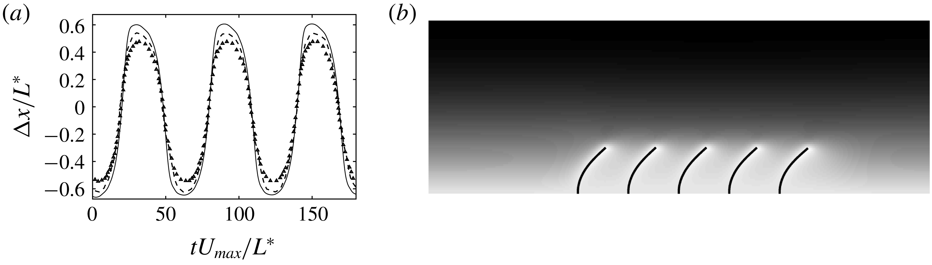
Figure 5. (a) Time history of the displacement of the filament free-end in an oscillatory flow (solid line) compared to the experimental (dashed line) and numerical (triangles) results by Pinelli et al. (Reference Pinelli, Omidyeganeh, Brücker, Revell, Sarkar and Alinovi2016). (b) Instantaneous visualisation of the row of filaments in the half-channel. The background colours indicate the streamwise velocity.
3 Flow configuration and suspension rheology
We study suspensions of flexible filaments at moderate volume fractions in a Couette flow, focusing on the role of inertia and flexibility on the suspension rheology. We consider stiff and flexible filaments suspended in a channel with the upper and lower walls moving with opposite velocities in the streamwise $x$
-direction; no-slip and no-penetration conditions are enforced on the moving walls, while periodicity is assumed in the homogeneous streamwise and spanwise directions. Initially, the filaments are randomly distributed in the channel. Figure 6 depicts the flow configuration and the coordinate system used in the present study, where the computational domain has size
$x$
-direction; no-slip and no-penetration conditions are enforced on the moving walls, while periodicity is assumed in the homogeneous streamwise and spanwise directions. Initially, the filaments are randomly distributed in the channel. Figure 6 depicts the flow configuration and the coordinate system used in the present study, where the computational domain has size $5L^{\ast }\times 5L^{\ast }\times 8L^{\ast }$
. The filament aspect ratio is set to
$5L^{\ast }\times 5L^{\ast }\times 8L^{\ast }$
. The filament aspect ratio is set to $r_{p}=1/16$
for all cases. In the present study, quantities are made dimensionless by the viscous scales, thus the non-dimensional bending stiffness is defined as
$r_{p}=1/16$
for all cases. In the present study, quantities are made dimensionless by the viscous scales, thus the non-dimensional bending stiffness is defined as
 $$\begin{eqnarray}\tilde{B}=\frac{B^{\ast }}{\unicode[STIX]{x1D707}\dot{\unicode[STIX]{x1D6FE}}L^{4}},\end{eqnarray}$$
and is related to the bending stiffness previously reported in (2.3) by
 $$\begin{eqnarray}\tilde{B}=\frac{\unicode[STIX]{x03C0}}{4}r_{p}^{2}Re\,B.\end{eqnarray}$$
The solid volume fraction of the suspension is
 $$\begin{eqnarray}\unicode[STIX]{x1D719}=\frac{n\unicode[STIX]{x03C0}r_{p}^{2}}{4V},\end{eqnarray}$$
where $n$
is the number of filaments in the computational box and
$n$
is the number of filaments in the computational box and $V$
the volume of the computational domain.
$V$
the volume of the computational domain.

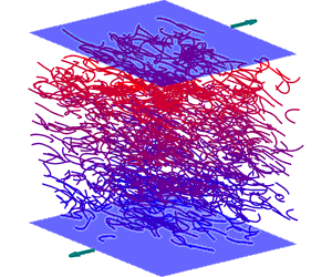
Figure 6. Schematic of the configuration and reference frame adopted in this study. The visualisation refers to a suspension of flexible filaments at $Re=10$
with volume fraction
$Re=10$
with volume fraction $\unicode[STIX]{x1D719}=0.018$
.
$\unicode[STIX]{x1D719}=0.018$
.
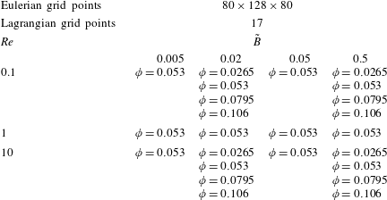
We perform a parametric study to assess the role of inertia, flexibility and volume fraction on the suspension flow. In particular, we vary the Reynolds number in the range $0.1\leqslant Re\leqslant 10$
, the bending rigidity in the range
$0.1\leqslant Re\leqslant 10$
, the bending rigidity in the range $0.005\leqslant \tilde{B}\leqslant 0.5$
and the volume fractions in the range
$0.005\leqslant \tilde{B}\leqslant 0.5$
and the volume fractions in the range $0.0265\leqslant \unicode[STIX]{x1D719}\leqslant 0.106$
; table 1 reports all the cases considered in the present work. In total, 24 configurations have been considered. For the filaments considered here, the so-called concentrated regime (Wu & Aidun Reference Wu and Aidun2010b
), when the filament–filament interactions become dominant in determining the macroscopic suspension behaviour, is reached for volume fractions
$0.0265\leqslant \unicode[STIX]{x1D719}\leqslant 0.106$
; table 1 reports all the cases considered in the present work. In total, 24 configurations have been considered. For the filaments considered here, the so-called concentrated regime (Wu & Aidun Reference Wu and Aidun2010b
), when the filament–filament interactions become dominant in determining the macroscopic suspension behaviour, is reached for volume fractions $\unicode[STIX]{x1D719}\geqslant 0.053$
(
$\unicode[STIX]{x1D719}\geqslant 0.053$
( $(n{L^{\ast }}^{3}/V)>1/r_{p}$
); in this case, suitable models for lubrication and contact forces are necessary.
$(n{L^{\ast }}^{3}/V)>1/r_{p}$
); in this case, suitable models for lubrication and contact forces are necessary.
In all our simulations, we use $80\times 128\times 80$
grid points in the streamwise, wall-normal and spanwise directions to discretise the computational domain, while
$80\times 128\times 80$
grid points in the streamwise, wall-normal and spanwise directions to discretise the computational domain, while $17$
Lagrangian points are used to describe each suspended filament, where the resolution has been chosen to properly resolve the cases with most flexible filaments. The time step necessary to properly capture the full filament dynamics is of the order of
$17$
Lagrangian points are used to describe each suspended filament, where the resolution has been chosen to properly resolve the cases with most flexible filaments. The time step necessary to properly capture the full filament dynamics is of the order of $\unicode[STIX]{x0394}t\approx 10^{-5}$
; note that the main time step constraint is determined by the elastic and lubrication forces in all the cases. We performed additional simulations with domain size, space and time resolution increased by a factor of
$\unicode[STIX]{x0394}t\approx 10^{-5}$
; note that the main time step constraint is determined by the elastic and lubrication forces in all the cases. We performed additional simulations with domain size, space and time resolution increased by a factor of $2$
for the most demanding cases and found that the difference in the suspension viscosity is lower than
$2$
for the most demanding cases and found that the difference in the suspension viscosity is lower than $2\,\%$
.
$2\,\%$
.
Table 1. Summary of the numerical simulations performed in this study. The table reports the Reynolds number $Re$
, the volume fraction
$Re$
, the volume fraction $\unicode[STIX]{x1D719}$
and the bending rigidity
$\unicode[STIX]{x1D719}$
and the bending rigidity $\tilde{B}$
of all cases presented in this study.
$\tilde{B}$
of all cases presented in this study.
3.1 Rheology of filament suspensions
The rheological behaviour of the suspensions is presented in terms of the relative viscosity
 $$\begin{eqnarray}\displaystyle \unicode[STIX]{x1D702}=\frac{\unicode[STIX]{x1D707}_{eff}}{\unicode[STIX]{x1D707}}, & & \displaystyle\end{eqnarray}$$
where $\unicode[STIX]{x1D707}$
is the viscosity of the carrier fluid and
$\unicode[STIX]{x1D707}$
is the viscosity of the carrier fluid and $\unicode[STIX]{x1D707}_{eff}$
is the effective viscosity of the suspension. The relative viscosity can be rewritten in terms of the bulk shear stress as
$\unicode[STIX]{x1D707}_{eff}$
is the effective viscosity of the suspension. The relative viscosity can be rewritten in terms of the bulk shear stress as
 $$\begin{eqnarray}\displaystyle \unicode[STIX]{x1D702}=1+\bar{\unicode[STIX]{x1D6F4}}_{xy}^{f}, & & \displaystyle\end{eqnarray}$$
where $\bar{\unicode[STIX]{x1D6F4}}_{xy}^{f}$
is the time and space average of the shear stress arising from the presence of the filaments, non-dimensionalised by the imposed shear rate
$\bar{\unicode[STIX]{x1D6F4}}_{xy}^{f}$
is the time and space average of the shear stress arising from the presence of the filaments, non-dimensionalised by the imposed shear rate $\dot{\unicode[STIX]{x1D6FE}}_{xy}$
and the viscosity
$\dot{\unicode[STIX]{x1D6FE}}_{xy}$
and the viscosity $\unicode[STIX]{x1D707}$
. The normal stress differences are used to describe the non-Newtonian behaviour of the suspension, and are defined as
$\unicode[STIX]{x1D707}$
. The normal stress differences are used to describe the non-Newtonian behaviour of the suspension, and are defined as
 $$\begin{eqnarray}\displaystyle N_{1}=\bar{\unicode[STIX]{x1D6F4}}_{xx}-\bar{\unicode[STIX]{x1D6F4}}_{yy},\quad N_{2}=\bar{\unicode[STIX]{x1D6F4}}_{yy}-\bar{\unicode[STIX]{x1D6F4}}_{zz}. & & \displaystyle\end{eqnarray}$$
To compute the total stress in the suspension and to differentiate all the different contributions, we follow the derivation first proposed by Batchelor (Reference Batchelor1970) for a suspension of rigid spherical particles and adapt it to the case of flexible filaments (see also Batchelor (Reference Batchelor1971) and Wu & Aidun (Reference Wu and Aidun2010a )). The dimensionless total stress reads as follows:
 $$\begin{eqnarray}\displaystyle \unicode[STIX]{x1D6F4}_{ij}=Re\left[\frac{1}{V}\int _{V-\unicode[STIX]{x1D6F4}V_{0}}\left(-P\unicode[STIX]{x1D6FF}_{ij}+\frac{2}{Re}\unicode[STIX]{x1D626}_{ij}\right)\text{d}V+\frac{1}{V}\sum \int _{V_{0}}\unicode[STIX]{x1D70E}_{ij},\text{d}V-\frac{1}{V}\int _{V}u_{i}^{\prime }u_{j}^{\prime }\,\text{d}V\right],\quad & & \displaystyle\end{eqnarray}$$
where $V$
is the total volume under investigation and
$V$
is the total volume under investigation and $V_{0}$
the volume of each filament;
$V_{0}$
the volume of each filament; $\unicode[STIX]{x1D626}_{ij}=(\unicode[STIX]{x2202}u_{i}/\unicode[STIX]{x2202}x_{j})+(\unicode[STIX]{x2202}u_{j}/\unicode[STIX]{x2202}x_{i})$
represents the strain rate tensor and
$\unicode[STIX]{x1D626}_{ij}=(\unicode[STIX]{x2202}u_{i}/\unicode[STIX]{x2202}x_{j})+(\unicode[STIX]{x2202}u_{j}/\unicode[STIX]{x2202}x_{i})$
represents the strain rate tensor and $\boldsymbol{u}^{\prime }$
the velocity fluctuations. The first term on the right-hand side of (3.7) represents the fluid bulk viscous stress tensor, the second term the stress generated by the fluid–solid interaction forces and the last term the stress generated by the velocity fluctuations in the fluid (the Reynolds stress tensor). We may write the total stress as the summation of the fluid and filament stress tensors as follows:
$\boldsymbol{u}^{\prime }$
the velocity fluctuations. The first term on the right-hand side of (3.7) represents the fluid bulk viscous stress tensor, the second term the stress generated by the fluid–solid interaction forces and the last term the stress generated by the velocity fluctuations in the fluid (the Reynolds stress tensor). We may write the total stress as the summation of the fluid and filament stress tensors as follows:
 $$\begin{eqnarray}\displaystyle \unicode[STIX]{x1D6F4}_{ij}=\bar{\unicode[STIX]{x1D6F4}}_{ij}^{0}+\bar{\unicode[STIX]{x1D6F4}}_{ij}^{f}, & & \displaystyle\end{eqnarray}$$
where
 $$\begin{eqnarray}\displaystyle \left.\begin{array}{@{}l@{}}\displaystyle \bar{\unicode[STIX]{x1D6F4}}_{ij}^{0}=\frac{Re}{V}\int _{V-\unicode[STIX]{x1D6F4}V_{0}}\left(-P\unicode[STIX]{x1D6FF}_{ij}+\frac{2}{Re}\unicode[STIX]{x1D626}_{ij}\right)\text{d}V,\\[13.0pt] \displaystyle \bar{\unicode[STIX]{x1D6F4}}_{ij}^{f}=\frac{Re}{V}\sum \int _{V_{0}}\unicode[STIX]{x1D70E}_{ij}\,\text{d}V-\frac{Re}{V}\int _{V}u_{i}^{\prime }u_{j}^{\prime }\,\text{d}V.\end{array}\right\} & & \displaystyle\end{eqnarray}$$
The fluid–solid interaction stress can be decomposed into two parts (Batchelor Reference Batchelor1970) as follows:
 $$\begin{eqnarray}\displaystyle \int _{V_{0}}\unicode[STIX]{x1D70E}_{ij}\,\text{d}V=\int _{A_{0}}\unicode[STIX]{x1D70E}_{ik}x_{j}n_{k}\,\text{d}A-\int _{V_{0}}\frac{\unicode[STIX]{x2202}\unicode[STIX]{x1D70E}_{ik}}{\unicode[STIX]{x2202}x_{k}}x_{j}\,\text{d}V, & & \displaystyle\end{eqnarray}$$
where $A_{0}$
represents the surface area of each filament. The first term is called the stresslet and the second term indicates the acceleration stress (Guazzelli & Morris Reference Guazzelli and Morris2011). For neutrally buoyant filaments, when the relative acceleration of fluid and the filament is zero, the second term in (3.10) is identically zero. Here
$A_{0}$
represents the surface area of each filament. The first term is called the stresslet and the second term indicates the acceleration stress (Guazzelli & Morris Reference Guazzelli and Morris2011). For neutrally buoyant filaments, when the relative acceleration of fluid and the filament is zero, the second term in (3.10) is identically zero. Here $\unicode[STIX]{x1D70E}_{ik}n_{k}$
is the force per unit area acting on the filaments (Batchelor Reference Batchelor1971), that for slender bodies can be rewritten as
$\unicode[STIX]{x1D70E}_{ik}n_{k}$
is the force per unit area acting on the filaments (Batchelor Reference Batchelor1971), that for slender bodies can be rewritten as
 $$\begin{eqnarray}\displaystyle \int _{A_{0}}\unicode[STIX]{x1D70E}_{ik}x_{j}n_{k}\,\text{d}A=-r_{p}^{2}\int _{L}\boldsymbol{F}_{i}x_{j}\,\text{d}s, & & \displaystyle\end{eqnarray}$$
where the term $r_{p}^{2}$
arises from choosing the linear density instead of the volume density as the scale for the fluid–solid interaction force. Finally, the filament stress is
$r_{p}^{2}$
arises from choosing the linear density instead of the volume density as the scale for the fluid–solid interaction force. Finally, the filament stress is
 $$\begin{eqnarray}\displaystyle \unicode[STIX]{x1D6F4}_{ij}^{f}=-\frac{Re{r_{p}}^{2}}{V}\sum \int _{L}\boldsymbol{F}_{i}x_{j}\,\text{d}s-\frac{Re}{V}\int _{V}u_{i}^{\prime }u_{j}^{\prime }\,\text{d}V. & & \displaystyle\end{eqnarray}$$
From the results of our simulations, we observe that the last term, related to the velocity fluctuations, is very small compared to the stresslet and can be thus neglected for the range of Reynolds numbers considered here. This is consistent with the behaviour of rigid particles for the same Reynolds numbers, $O(10)$
, as shown in Alghalibi et al. (Reference Alghalibi, Lashgari, Brandt and Hormozi2018).
$O(10)$
, as shown in Alghalibi et al. (Reference Alghalibi, Lashgari, Brandt and Hormozi2018).
4 Results
4.1 Suspensions of rigid fibres in shear flow
We start our analysis by comparing the relative viscosity of concentrated rigid fibre suspensions at negligible flow inertia obtained from our simulations with the theoretical, numerical and experimental results reported in the literature. In particular, we discuss here the role of the short-range friction model for fibres. Our results are obtained for Reynolds number, $Re=0.1$
, and with flexibility,
$Re=0.1$
, and with flexibility, $\tilde{B}=0.5$
, which properly reproduces rigid filaments. The data are presented in figure 7 showing that results from the present numerical simulations are within the range predicted by the numerical and experimental results in the literature, as well as the theoretical prediction of Liu et al. (Reference Liu, Zhang, Wang and Liu2004) for a suspension of fibres rotating only in the shear plane. In order to show the importance of the lubrication correction, we also display results obtained without it: in this case the suspension viscosity is strongly under-predicted, especially at high volume fractions, resulting in large differences between our results and the experimental data. The test confirms that within the framework of our numerical scheme and with the chosen grid resolution, the short-range interactions are indeed important when considering concentrated regimes.
$\tilde{B}=0.5$
, which properly reproduces rigid filaments. The data are presented in figure 7 showing that results from the present numerical simulations are within the range predicted by the numerical and experimental results in the literature, as well as the theoretical prediction of Liu et al. (Reference Liu, Zhang, Wang and Liu2004) for a suspension of fibres rotating only in the shear plane. In order to show the importance of the lubrication correction, we also display results obtained without it: in this case the suspension viscosity is strongly under-predicted, especially at high volume fractions, resulting in large differences between our results and the experimental data. The test confirms that within the framework of our numerical scheme and with the chosen grid resolution, the short-range interactions are indeed important when considering concentrated regimes.

Figure 7. Relative viscosity versus solid volume fraction for suspensions of rigid fibres. The red and blue filled symbols refer to the present numerical results with and without the lubrication correction. The open symbols denote the experimental data of Blakeney (Reference Blakeney1966), while the filled black symbols denote the experimental data of Bibbó (Reference Bibbó1987). The $+$
symbols show the numerical results by Lindström & Uesaka (Reference Lindström and Uesaka2008) and
$+$
symbols show the numerical results by Lindström & Uesaka (Reference Lindström and Uesaka2008) and $\times$
those by Lindström & Uesaka (Reference Lindström and Uesaka2008), including contact friction between filaments. The solid line represents the theoretical prediction of Liu et al. (Reference Liu, Zhang, Wang and Liu2004) for a suspension of fibres rotating only in the shear plane.
$\times$
those by Lindström & Uesaka (Reference Lindström and Uesaka2008), including contact friction between filaments. The solid line represents the theoretical prediction of Liu et al. (Reference Liu, Zhang, Wang and Liu2004) for a suspension of fibres rotating only in the shear plane.
4.2 Suspensions of flexible filaments at fixed volume fraction
We now analyse the suspension behaviour at fixed volume fraction, $\unicode[STIX]{x1D719}=0.053$
, and vary the Reynolds number and filament flexibility. First, we report in figure 8 the dependence of the relative shear viscosity of the suspension on the bending rigidity (a) and the Reynolds number (b). Figure 8(a) shows that the viscosity increases with the bending rigidity, i.e. the viscosity decreases as the filaments are more flexible. This result is in agreement with the simulations by Switzer III & Klingenberg (Reference Switzer III and Klingenberg2003) and Sepehr et al. (Reference Sepehr, Carreau, Moan and Ausias2004) for flexible fibres, and also to the results pertaining to the case of deformable particles, capsules and droplets (see e.g. Reasor, Clausen & Aidun (Reference Reasor, Clausen and Aidun2013), Matsunaga et al. (Reference Matsunaga, Imai, Yamaguchi and Ishikawa2016), Rosti & Brandt (Reference Rosti and Brandt2018) and Rosti, De Vita & Brandt (Reference Rosti, De Vita and Brandt2019a
)). These observations are in contrast with the results of Wu & Aidun (Reference Wu and Aidun2010b
) where larger viscosities are obtained for more flexible cases. This difference can be explained by the different physical objects under consideration: Joung et al. (Reference Joung, Phan-Thien and Fan2001) and Wu & Aidun (Reference Wu and Aidun2010b
) considered chains of interconnected rigid particles which can twist and bend at their joints, while we consider continuously flexible filaments that can only bend. Suspensions of elastic elongated objects can therefore display different behaviour: viscosity decreasing with deformability (Switzer III & Klingenberg Reference Switzer III and Klingenberg2003; Sepehr et al.
Reference Sepehr, Carreau, Moan and Ausias2004) or increasing with it (Joung et al.
Reference Joung, Phan-Thien and Fan2001; Wu & Aidun Reference Wu and Aidun2010b
). Note also that, although Switzer III & Klingenberg (Reference Switzer III and Klingenberg2003) and Sepehr et al. (Reference Sepehr, Carreau, Moan and Ausias2004) adopt a model similar to the one used by Wu & Aidun (Reference Wu and Aidun2010b
), they observe the same behaviour as in our results which may be explained by the different aspect ratio considered; indeed, the former authors considered fibres whose aspect ratio is at least
$\unicode[STIX]{x1D719}=0.053$
, and vary the Reynolds number and filament flexibility. First, we report in figure 8 the dependence of the relative shear viscosity of the suspension on the bending rigidity (a) and the Reynolds number (b). Figure 8(a) shows that the viscosity increases with the bending rigidity, i.e. the viscosity decreases as the filaments are more flexible. This result is in agreement with the simulations by Switzer III & Klingenberg (Reference Switzer III and Klingenberg2003) and Sepehr et al. (Reference Sepehr, Carreau, Moan and Ausias2004) for flexible fibres, and also to the results pertaining to the case of deformable particles, capsules and droplets (see e.g. Reasor, Clausen & Aidun (Reference Reasor, Clausen and Aidun2013), Matsunaga et al. (Reference Matsunaga, Imai, Yamaguchi and Ishikawa2016), Rosti & Brandt (Reference Rosti and Brandt2018) and Rosti, De Vita & Brandt (Reference Rosti, De Vita and Brandt2019a
)). These observations are in contrast with the results of Wu & Aidun (Reference Wu and Aidun2010b
) where larger viscosities are obtained for more flexible cases. This difference can be explained by the different physical objects under consideration: Joung et al. (Reference Joung, Phan-Thien and Fan2001) and Wu & Aidun (Reference Wu and Aidun2010b
) considered chains of interconnected rigid particles which can twist and bend at their joints, while we consider continuously flexible filaments that can only bend. Suspensions of elastic elongated objects can therefore display different behaviour: viscosity decreasing with deformability (Switzer III & Klingenberg Reference Switzer III and Klingenberg2003; Sepehr et al.
Reference Sepehr, Carreau, Moan and Ausias2004) or increasing with it (Joung et al.
Reference Joung, Phan-Thien and Fan2001; Wu & Aidun Reference Wu and Aidun2010b
). Note also that, although Switzer III & Klingenberg (Reference Switzer III and Klingenberg2003) and Sepehr et al. (Reference Sepehr, Carreau, Moan and Ausias2004) adopt a model similar to the one used by Wu & Aidun (Reference Wu and Aidun2010b
), they observe the same behaviour as in our results which may be explained by the different aspect ratio considered; indeed, the former authors considered fibres whose aspect ratio is at least $5$
times smaller than those studied by Wu & Aidun (Reference Wu and Aidun2010b
). Note also that the relative viscosity changes with the flexibility in a very similar way to shear thinning fluids: with decreasing
$5$
times smaller than those studied by Wu & Aidun (Reference Wu and Aidun2010b
). Note also that the relative viscosity changes with the flexibility in a very similar way to shear thinning fluids: with decreasing $\tilde{B}$
, the relative viscosity approaches a constant value while the other plateau for high
$\tilde{B}$
, the relative viscosity approaches a constant value while the other plateau for high $\tilde{B}$
is not captured in the range of rigidity considered in this work.
$\tilde{B}$
is not captured in the range of rigidity considered in this work.

Figure 8. Relative viscosity of filament suspensions versus (a) the filament bending rigidity and (b) the Reynolds number. The suspension volume fraction is fixed to $\unicode[STIX]{x1D719}=0.053$
for all cases.
$\unicode[STIX]{x1D719}=0.053$
for all cases.
Figure 8(b) displays the same data of figure 8(a), now as a function of the Reynolds number, in order to highlight how inertia affects the suspension viscosity. We observe that $\unicode[STIX]{x1D702}$
increases with Reynolds number, especially for the most stiff cases; this indicates that inertial effects are more evident for rigid rods than for flexible filaments.
$\unicode[STIX]{x1D702}$
increases with Reynolds number, especially for the most stiff cases; this indicates that inertial effects are more evident for rigid rods than for flexible filaments.
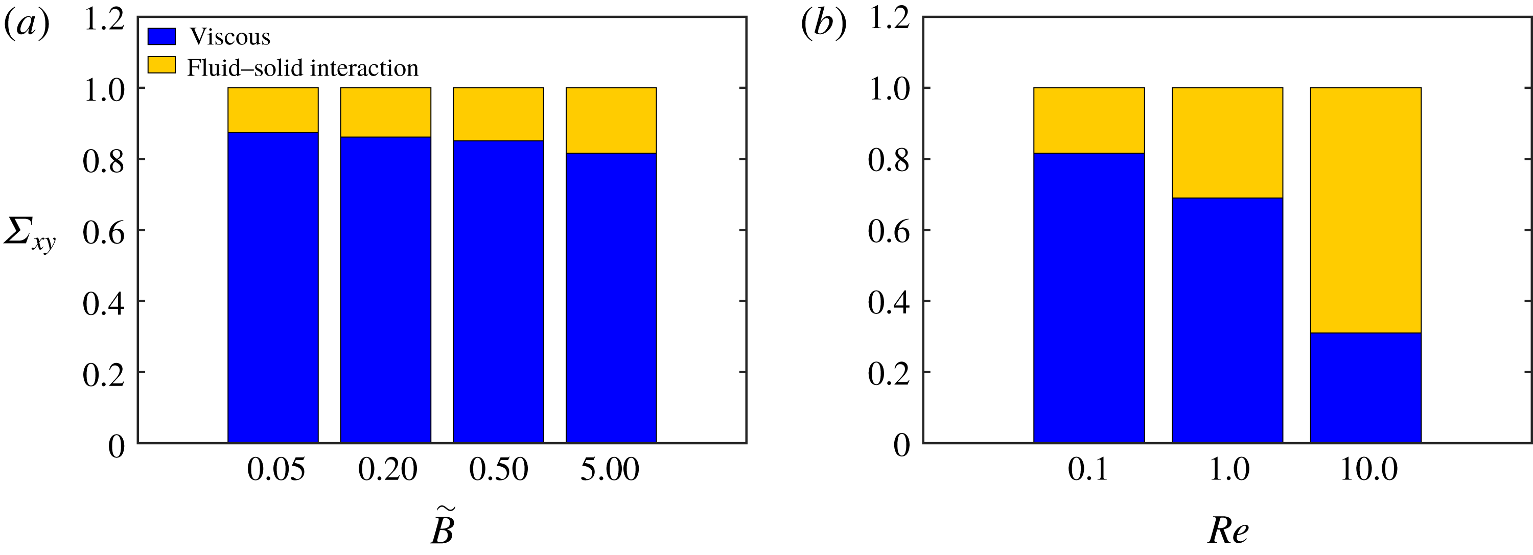
Figure 9. Stress budget. Relative contributions to the total shear stress from the viscous and fluid–solid interaction stresses versus (a) the filament bending rigidity at a fixed Reynolds number equal to $Re=0.1$
and (b) for different Reynolds numbers and fixed bending rigidity
$Re=0.1$
and (b) for different Reynolds numbers and fixed bending rigidity $\tilde{B}=0.5$
. The volume fraction is equal to
$\tilde{B}=0.5$
. The volume fraction is equal to $\unicode[STIX]{x1D719}=0.053$
. Note that the total shear stress is normalised with the total shear stress of each case, cf. figure 8 for the absolute values.
$\unicode[STIX]{x1D719}=0.053$
. Note that the total shear stress is normalised with the total shear stress of each case, cf. figure 8 for the absolute values.
To better understand the rheological behaviour of the suspensions we next examine the different contributions to the total shear stress, as derived in the previous section, see (3.12). Figure 9(a) reports the relative contribution of the viscous and fluid–solid interaction stresses to the total shear stress for the case with low inertia, $Re=0.1$
, and for different values of
$Re=0.1$
, and for different values of $\tilde{B}$
, whereas figure 9(b) considers the behaviour for different Reynolds numbers at a fixed bending rigidity,
$\tilde{B}$
, whereas figure 9(b) considers the behaviour for different Reynolds numbers at a fixed bending rigidity, $\tilde{B}=0.5$
. Note that the Reynolds stresses are negligible also at the highest Reynolds numbers considered and are therefore not displayed in figure 9.
$\tilde{B}=0.5$
. Note that the Reynolds stresses are negligible also at the highest Reynolds numbers considered and are therefore not displayed in figure 9.
Figure 9(a) clearly reveals that the contribution to the total stress from the suspended filaments reduces when decreasing the fibre rigidity; on the other hand, the results in figure 9(b) show that changes of the Reynolds number strongly affect the suspension and that the filament contribution increases with inertia and eventually becomes the dominant effect at $Re=10$
, where the fluid–solid interaction stress is
$Re=10$
, where the fluid–solid interaction stress is $66\,\%$
of the total stress. Thus, we can attribute the large increase of the suspension viscosity observed in figure 8(b) to the fluid–solid interaction forces. Interestingly, the increase of the filament stress with the Reynolds number is more evident from
$66\,\%$
of the total stress. Thus, we can attribute the large increase of the suspension viscosity observed in figure 8(b) to the fluid–solid interaction forces. Interestingly, the increase of the filament stress with the Reynolds number is more evident from $Re=1$
to
$Re=1$
to $Re=10$
indicating a strong nonlinear behaviour, as also seen in the relative viscosity curve. Note that the same trend is observed also for the other values of
$Re=10$
indicating a strong nonlinear behaviour, as also seen in the relative viscosity curve. Note that the same trend is observed also for the other values of $\tilde{B}$
under investigation, with the increase of the fluid–solid interaction term being higher for stiff fibres (data not shown). The increase of the stress component due to the fluid–solid interaction can be related to the increase in the drag force experienced by the filaments at finite inertia, similarly to what is observed for cylinders and spheres (Fornberg Reference Fornberg1980).
$\tilde{B}$
under investigation, with the increase of the fluid–solid interaction term being higher for stiff fibres (data not shown). The increase of the stress component due to the fluid–solid interaction can be related to the increase in the drag force experienced by the filaments at finite inertia, similarly to what is observed for cylinders and spheres (Fornberg Reference Fornberg1980).
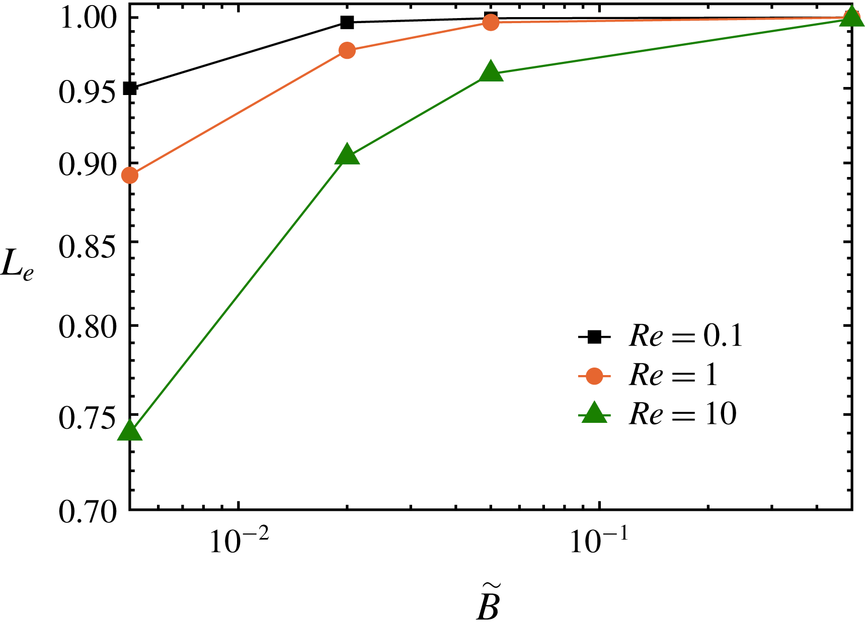
Figure 10. Time and ensemble average end-to-end distance $L_{e}$
of the suspended filaments as a function of their bending rigidity
$L_{e}$
of the suspended filaments as a function of their bending rigidity $\tilde{B}$
for the different Reynolds numbers investigated, as indicated in the legend.
$\tilde{B}$
for the different Reynolds numbers investigated, as indicated in the legend.
To examine the filament dynamics and their deformation, we now consider the mean distance between the two ends of each filament, where the average is performed over time and the number of filaments. The data pertaining to all the different cases under investigation are shown in figure 10. The figure indicates that the end-to-end distance increases as the bending stiffness is increased, i.e. the filaments’ deformation decreases for larger values of $\tilde{B}$
. Moreover, the average end-to-end distance decreases with the Reynolds number, i.e. the filaments deform more when increasing the inertial effects. These observations are consistent with the results of the relative viscosity and stress budget discussed above, as we have reported larger filament stresses for the stiff cases and larger suspension viscosity at finite Reynolds number.
$\tilde{B}$
. Moreover, the average end-to-end distance decreases with the Reynolds number, i.e. the filaments deform more when increasing the inertial effects. These observations are consistent with the results of the relative viscosity and stress budget discussed above, as we have reported larger filament stresses for the stiff cases and larger suspension viscosity at finite Reynolds number.

Figure 11. Snapshots of co-located filaments projected onto the shear plane in statistically steady state for (a) $\tilde{B}=0.5,Re=0.1$
(b)
$\tilde{B}=0.5,Re=0.1$
(b) $\tilde{B}=0.005,Re=0.1$
and (c)
$\tilde{B}=0.005,Re=0.1$
and (c) $\tilde{B}=0.005,Re=10$
. The solid red line is the circle with diameter equal to the filament’s length whereas the blue dashed line represents the circle with diameter equal to the mean end-to-end distance reported in figure 10. The black circle represents the minimum end-to-end distance for each case and the black solid lines denote the average orientation with respect to the walls. Note that the three lines coincide in the case of rigid fibres in (a). The orientation angles for the cases with flexible fibres are computed on the line connecting the two ends of the filament.
$\tilde{B}=0.005,Re=10$
. The solid red line is the circle with diameter equal to the filament’s length whereas the blue dashed line represents the circle with diameter equal to the mean end-to-end distance reported in figure 10. The black circle represents the minimum end-to-end distance for each case and the black solid lines denote the average orientation with respect to the walls. Note that the three lines coincide in the case of rigid fibres in (a). The orientation angles for the cases with flexible fibres are computed on the line connecting the two ends of the filament.
In order to visualise the filaments’ deformation in the suspension flow at the statistically steady state, we display them co-located with their centre positioned at the origin of the axis, i.e. we move their centre to (0,0,0) and plot all filaments on the same graph. These are shown in figure 11 where we display the projection of the filament configuration in the shear plane for three representative cases: a stiff ( $\tilde{B}=0.5$
) and a flexible case (
$\tilde{B}=0.5$
) and a flexible case ( $\tilde{B}=0.005$
) at negligible inertia (low Reynolds number,
$\tilde{B}=0.005$
) at negligible inertia (low Reynolds number, $Re=0.1$
) and a flexible case at high Reynolds number
$Re=0.1$
) and a flexible case at high Reynolds number $\tilde{B}=0.005$
and
$\tilde{B}=0.005$
and $Re=10$
. In figure 11, the solid red line is the circle with diameter equal to the filament’s length whereas the blue dashed line represents the circle with diameter equal to the mean end-to-end distance reported in figure 10; the black circle represents the minimum end-to-end distance for each case and the solid line the mean orientation of the filaments. For
$Re=10$
. In figure 11, the solid red line is the circle with diameter equal to the filament’s length whereas the blue dashed line represents the circle with diameter equal to the mean end-to-end distance reported in figure 10; the black circle represents the minimum end-to-end distance for each case and the solid line the mean orientation of the filaments. For $\tilde{B}=0.5$
and
$\tilde{B}=0.5$
and $Re=0.1$
(low inertia and rigid-like filaments) (a), the majority of the filaments exhibit negligible bending and indeed the mean end-to-end distance is very close to the fibre length. Larger deformations are observed for
$Re=0.1$
(low inertia and rigid-like filaments) (a), the majority of the filaments exhibit negligible bending and indeed the mean end-to-end distance is very close to the fibre length. Larger deformations are observed for $\tilde{B}=0.005$
and
$\tilde{B}=0.005$
and $Re=0.1$
(figure 11
b), with a minimum end-to-end distance lower than that in (a). Finally, for
$Re=0.1$
(figure 11
b), with a minimum end-to-end distance lower than that in (a). Finally, for $\tilde{B}=0.005$
and
$\tilde{B}=0.005$
and $Re=10$
(figure 11
c) the filaments exhibit a substantial bending with a smaller minimum of the instantaneous end-to-end distance. Note also that the filaments’ deformation is larger for orientation angles around
$Re=10$
(figure 11
c) the filaments exhibit a substantial bending with a smaller minimum of the instantaneous end-to-end distance. Note also that the filaments’ deformation is larger for orientation angles around $135^{\circ }$
and
$135^{\circ }$
and $315^{\circ }$
with respect to the flow direction i.e. in the compression region of the shear plane, which can be attributed to the maximum acceleration achieved at this inclination and to the buckling of the filaments under compressive forces (Becker & Shelley Reference Becker and Shelley2001; Tornberg & Shelley Reference Tornberg and Shelley2004). For angles close to
$315^{\circ }$
with respect to the flow direction i.e. in the compression region of the shear plane, which can be attributed to the maximum acceleration achieved at this inclination and to the buckling of the filaments under compressive forces (Becker & Shelley Reference Becker and Shelley2001; Tornberg & Shelley Reference Tornberg and Shelley2004). For angles close to $45^{\circ }$
and
$45^{\circ }$
and $225^{\circ }$
(the extension region of the shear plane) the acceleration is small as the filaments are aligned to the imposed shear with the hydrodynamic forces working to extend the filaments, which results in the filaments exhibiting small deformations.
$225^{\circ }$
(the extension region of the shear plane) the acceleration is small as the filaments are aligned to the imposed shear with the hydrodynamic forces working to extend the filaments, which results in the filaments exhibiting small deformations.

Figure 12. Bending energy $\tilde{E_{b}}$
as a function of the filament’s bending stiffness
$\tilde{E_{b}}$
as a function of the filament’s bending stiffness $\tilde{B}$
for the different Reynolds numbers indicated in the legend.
$\tilde{B}$
for the different Reynolds numbers indicated in the legend.
In filament suspensions, there is an exchange between fluid kinetic energy and filament bending energy, where the amount of bending energy directly affects the suspension’s bulk elasticity. It is therefore interesting to study the mean filament bending energy, defined as follows:
 $$\begin{eqnarray}\displaystyle \tilde{E_{b}}=\frac{1}{n}\tilde{B}\sum \mathop{\int }_{0}^{1}\left\Vert \frac{\unicode[STIX]{x2202}^{2}\boldsymbol{X}}{\unicode[STIX]{x2202}s^{2}}\right\Vert ^{2}\,\text{d}s. & & \displaystyle\end{eqnarray}$$
Equation (4.1) shows that the energy depends linearly on the bending rigidity $\tilde{B}$
and quadratically on the filament curvature
$\tilde{B}$
and quadratically on the filament curvature $\Vert \unicode[STIX]{x2202}^{2}\boldsymbol{X}/\unicode[STIX]{x2202}s^{2}\Vert$
; this implies that the bending energy tends to zero for very soft (
$\Vert \unicode[STIX]{x2202}^{2}\boldsymbol{X}/\unicode[STIX]{x2202}s^{2}\Vert$
; this implies that the bending energy tends to zero for very soft ( $\tilde{B}\rightarrow 0$
) and very stiff (
$\tilde{B}\rightarrow 0$
) and very stiff ( $\Vert \unicode[STIX]{x2202}^{2}\boldsymbol{X}/\unicode[STIX]{x2202}s^{2}\Vert \rightarrow 0$
) cases and a maximum should exist for intermediate values of
$\Vert \unicode[STIX]{x2202}^{2}\boldsymbol{X}/\unicode[STIX]{x2202}s^{2}\Vert \rightarrow 0$
) cases and a maximum should exist for intermediate values of $\tilde{B}$
. The bending energy of all the different suspensions under consideration is displayed in figure 12; the peak corresponding to the maximum elastic energy of the suspension shifts to low
$\tilde{B}$
. The bending energy of all the different suspensions under consideration is displayed in figure 12; the peak corresponding to the maximum elastic energy of the suspension shifts to low $\tilde{B}$
when the Reynolds number decreases and, as expected, the bending energy approaches zero for the stiffest cases. It can also be inferred from the figure that for a fixed rigidity the bending energy increases with the Reynolds number, especially from
$\tilde{B}$
when the Reynolds number decreases and, as expected, the bending energy approaches zero for the stiffest cases. It can also be inferred from the figure that for a fixed rigidity the bending energy increases with the Reynolds number, especially from $Re=1$
to
$Re=1$
to $Re=10$
, due to the larger filament deformation.
$Re=10$
, due to the larger filament deformation.

Figure 13. First normal stress difference $N_{1}$
as a function of the bending rigidity
$N_{1}$
as a function of the bending rigidity $\tilde{B}$
for the different Reynolds numbers under investigation. The volume fraction is fixed to
$\tilde{B}$
for the different Reynolds numbers under investigation. The volume fraction is fixed to $\unicode[STIX]{x1D719}=0.053$
.
$\unicode[STIX]{x1D719}=0.053$
.
As mentioned before, the bending energy can be directly related to the viscoelastic behaviour of the filament suspension. In order to quantify this effect, we examine the first normal stress difference for the different Reynolds numbers and bending rigidities under investigation, see figure 13. As expected for a viscoelastic suspension, the first normal stress difference is positive, similar to what was found in the case of polymers, deformable particles and capsules (Mewis & Wagner Reference Mewis and Wagner2012; Matsunaga et al.
Reference Matsunaga, Imai, Yamaguchi and Ishikawa2016; Rosti & Brandt Reference Rosti and Brandt2018; Shahmardi et al.
Reference Shahmardi, Zade, Ardekani, Poole, Lundell, Rosti and Brandt2019). Interestingly, the trend in figure 13 is similar to that of the bending energy, with the first normal stress difference increasing with the flow inertia; furthermore, we note the presence of a maximum of $N_{1}$
, whose location is shifting to larger values of
$N_{1}$
, whose location is shifting to larger values of $\tilde{B}$
when the Reynolds number is increased. In order to capture accurately the location of the maximum, we performed additional simulations for
$\tilde{B}$
when the Reynolds number is increased. In order to capture accurately the location of the maximum, we performed additional simulations for $Re=1$
and
$Re=1$
and $10$
. The filament suspension exhibits the highest first normal stress difference at around
$10$
. The filament suspension exhibits the highest first normal stress difference at around $\tilde{B}=0,05$
for
$\tilde{B}=0,05$
for $Re=10$
and around
$Re=10$
and around $\tilde{B}=0,005$
for
$\tilde{B}=0,005$
for $Re=1$
, thus suggesting that the value of
$Re=1$
, thus suggesting that the value of $\tilde{B}$
for which the maximum first normal stress difference is achieved scales approximately with the Reynolds number. Note that for
$\tilde{B}$
for which the maximum first normal stress difference is achieved scales approximately with the Reynolds number. Note that for $Re=0.1$
the peak of the first normal stress difference is expected for values of
$Re=0.1$
the peak of the first normal stress difference is expected for values of $\tilde{B}$
below those considered here.
$\tilde{B}$
below those considered here.

Figure 14. Root mean square of the streamwise $u^{\prime }$
and wall-normal
$u^{\prime }$
and wall-normal $v^{\prime }$
velocity fluctuations integrated across the channel width as a function of the filament bending stiffness
$v^{\prime }$
velocity fluctuations integrated across the channel width as a function of the filament bending stiffness $\tilde{B}$
for different values of the Reynolds number
$\tilde{B}$
for different values of the Reynolds number $Re$
, as indicated in the figure.
$Re$
, as indicated in the figure.
Before concluding this section, we consider the root mean square of the fluid velocity fluctuations induced by the presence of the filament. The integral across the channel of the streamwise and wall-normal velocity fluctuations is displayed in figure 14. As expected, we note that the velocity fluctuations increase with the Reynolds number, due to larger fluid–solid interaction forces as $Re$
increases. The magnitude of these fluctuations is approximately independent of the bending rigidity
$Re$
increases. The magnitude of these fluctuations is approximately independent of the bending rigidity $\tilde{B}$
for the different Reynolds numbers examined, except for a small peak corresponding to the maximum of the first normal stress difference, which is more evident at finite inertia. This weak dependency on the rigidity suggests that, for the parameters considered in this study, fluid velocity fluctuations are mainly induced by filament rotation.
$\tilde{B}$
for the different Reynolds numbers examined, except for a small peak corresponding to the maximum of the first normal stress difference, which is more evident at finite inertia. This weak dependency on the rigidity suggests that, for the parameters considered in this study, fluid velocity fluctuations are mainly induced by filament rotation.
4.3 Rheology when varying the filament volume fraction
In this section we investigate the effect of the filament volume fraction at $Re=0.1$
and
$Re=0.1$
and $Re=10$
for two different values of rigidity,
$Re=10$
for two different values of rigidity, $\tilde{B}=0.5$
and
$\tilde{B}=0.5$
and $\tilde{B}=0.02$
. The former case is chosen as representative of the behaviour of rigid fibres as the deformation is negligible also at the highest Reynolds number considered.
$\tilde{B}=0.02$
. The former case is chosen as representative of the behaviour of rigid fibres as the deformation is negligible also at the highest Reynolds number considered.

Figure 15. Relative viscosity and first normal stress difference as a function of the filament volume fraction for different Reynolds numbers and flexibilities as indicated in the legend.
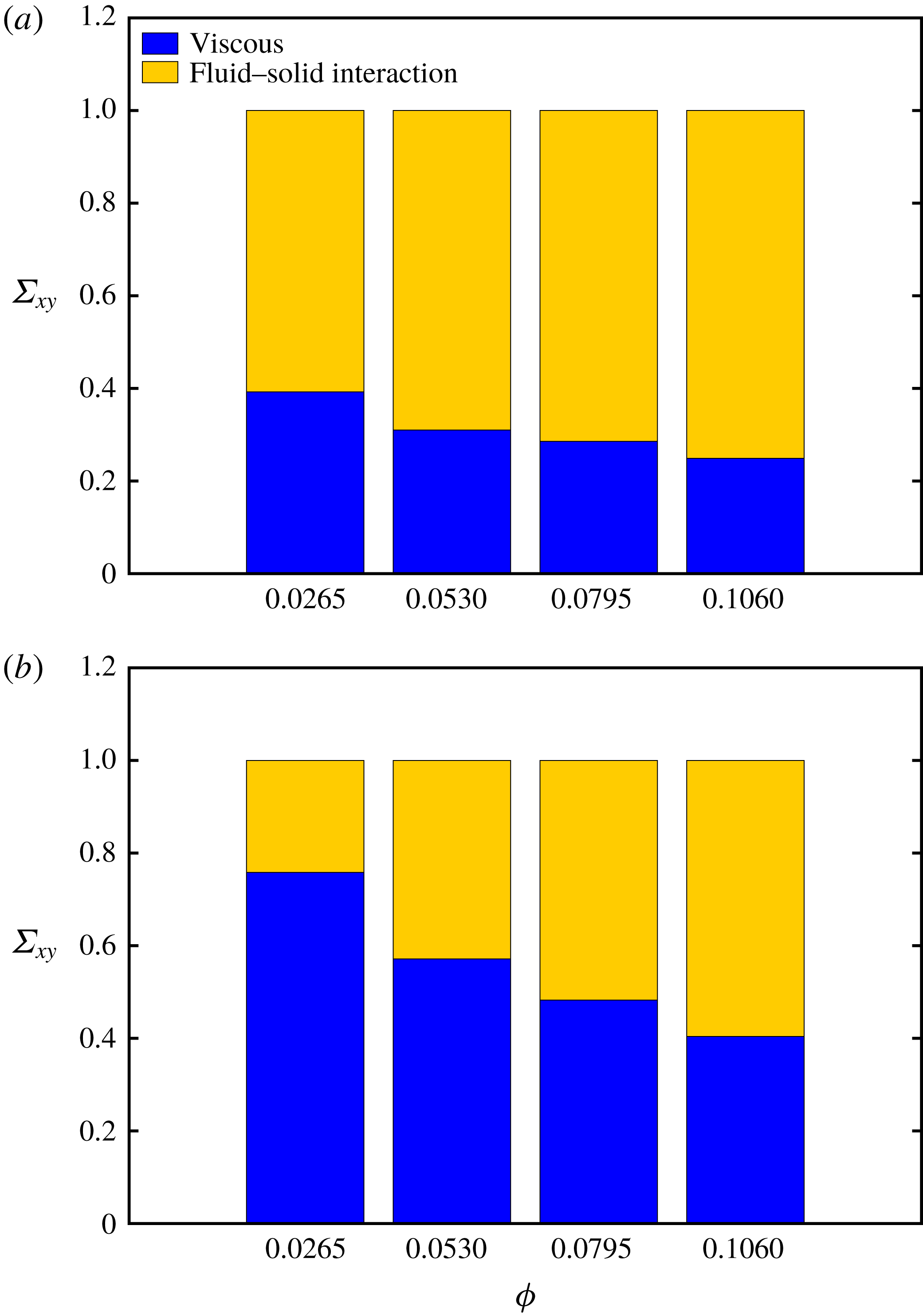
Figure 16. Stress budget. Relative contributions to the total shear stress from the viscous and fluid–solid interaction stresses versus the filament volume fraction at $Re=10$
, for (a)
$Re=10$
, for (a) $\tilde{B}=0.5$
and (b)
$\tilde{B}=0.5$
and (b) $\tilde{B}=0.02$
. Note that the total shear stress is normalised with the total shear stress of each case, cf. figure 15 for the absolute values.
$\tilde{B}=0.02$
. Note that the total shear stress is normalised with the total shear stress of each case, cf. figure 15 for the absolute values.
In figure 15 we present the suspension rheological behaviour in terms of relative viscosity and first normal stress difference. The data in figure 15 clearly show that the relative viscosity increases with the volume fraction except for the cases at the two highest $\unicode[STIX]{x1D719}$
for negligible inertia and rigid filaments,
$\unicode[STIX]{x1D719}$
for negligible inertia and rigid filaments, $Re=0.1$
and
$Re=0.1$
and $\tilde{B}=0.5$
. In this case, we report a slight decrease of the effective viscosity which we explain by the orientation angle of the filaments. Indeed, by increasing the volume fraction from
$\tilde{B}=0.5$
. In this case, we report a slight decrease of the effective viscosity which we explain by the orientation angle of the filaments. Indeed, by increasing the volume fraction from $7.9\,\%$
to
$7.9\,\%$
to $10.6\,\%$
, filaments become more aligned with the mean flow which results in lower viscosity and also reduced normal stress difference. A similar reduction has also been observed by Lindström & Uesaka (Reference Lindström and Uesaka2008). Furthermore, we note only a small difference in the relative viscosity for the two cases with different bending rigidities at negligible inertia,
$10.6\,\%$
, filaments become more aligned with the mean flow which results in lower viscosity and also reduced normal stress difference. A similar reduction has also been observed by Lindström & Uesaka (Reference Lindström and Uesaka2008). Furthermore, we note only a small difference in the relative viscosity for the two cases with different bending rigidities at negligible inertia, $Re=0.1$
, which can be attributed to the small difference in the mean filament deformation, as will be discussed later. At finite inertia,
$Re=0.1$
, which can be attributed to the small difference in the mean filament deformation, as will be discussed later. At finite inertia, $Re=10$
, the suspensions of more flexible filaments display lower viscosity, confirming the decrease with the flexibility discussed above.
$Re=10$
, the suspensions of more flexible filaments display lower viscosity, confirming the decrease with the flexibility discussed above.
The first normal stress difference, see figure 15(b), also increases with the volume fraction, more visibly at the highest Reynolds number considered, $Re=10$
. The first normal stress difference is larger for the suspension of most flexible filaments at higher Reynolds numbers, while it increases slowly at larger
$Re=10$
. The first normal stress difference is larger for the suspension of most flexible filaments at higher Reynolds numbers, while it increases slowly at larger $\unicode[STIX]{x1D719}$
and
$\unicode[STIX]{x1D719}$
and $\tilde{B}=0.5$
. At low Reynolds numbers, the values of
$\tilde{B}=0.5$
. At low Reynolds numbers, the values of $N_{1}$
are similar for the suspensions of rigid and deformable filament, and a difference is only visible at the highest
$N_{1}$
are similar for the suspensions of rigid and deformable filament, and a difference is only visible at the highest $\unicode[STIX]{x1D719}$
considered, which can be related to the formation of a micro-structure in the suspensions so that the filaments have lower mobility as further discussed below.
$\unicode[STIX]{x1D719}$
considered, which can be related to the formation of a micro-structure in the suspensions so that the filaments have lower mobility as further discussed below.
The stress budget pertaining to the cases at different volume fraction $\unicode[STIX]{x1D719}$
is displayed in figure 16 where we report the relative contribution from viscous and elastic stresses (the absolute values of the shear viscosity being depicted in figure 15). As expected from the results above, the contribution from the fluid–solid interaction force increases with the filament rigidity and volume fraction.
$\unicode[STIX]{x1D719}$
is displayed in figure 16 where we report the relative contribution from viscous and elastic stresses (the absolute values of the shear viscosity being depicted in figure 15). As expected from the results above, the contribution from the fluid–solid interaction force increases with the filament rigidity and volume fraction.
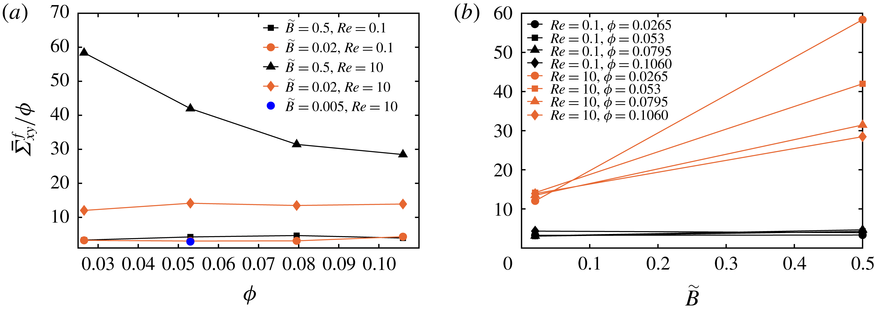
Figure 17. Filament contribution to the total shear stress scaled with the volume fraction as a function of (a) volume fraction and (b) bending stiffness.

Figure 18. Average orientation angle with the wall for the most stiff filaments in suspensions with $Re=10$
and
$Re=10$
and $\tilde{B}=0.5$
.
$\tilde{B}=0.5$
.
Figure 17 represents the variation of the filament contribution to the average total shear stress scaled by the volume fraction. Note that this contribution also includes lubrication and collision forces. It can be observed in figure 17(a) that at low Reynolds number, the contribution is proportional to the volume fraction both for rigid and flexible filaments, meaning that filament–filament interactions are negligible and that deformation is weak, to give a visible effect. The blue dot in figure 17(a), pertaining to the suspensions with most flexible filaments at $\unicode[STIX]{x1D719}=5.3\,\%$
(see previous section), also suggests that the filament stress decreases for more deformable objects, although this effect is still small for the cases considered here at negligible inertia. When inertia is important,
$\unicode[STIX]{x1D719}=5.3\,\%$
(see previous section), also suggests that the filament stress decreases for more deformable objects, although this effect is still small for the cases considered here at negligible inertia. When inertia is important, $Re=10$
, the filament stress contribution increases, as shown by the global shear viscosity in figure 15(a), while the linear dependence on the volume fraction is only observed for the most deformable filaments. On the contrary, the contribution decreases with the volume fraction for the rigid filaments; this is due to the fact that rigid filaments tend to align in the shear direction (see figure 18), which reduces the importance of the short-range interactions. In this case, the filaments move almost as an aggregate, with decreased relative motion. The same data are depicted in figure 17(b), as a function of the bending stiffness. At
$Re=10$
, the filament stress contribution increases, as shown by the global shear viscosity in figure 15(a), while the linear dependence on the volume fraction is only observed for the most deformable filaments. On the contrary, the contribution decreases with the volume fraction for the rigid filaments; this is due to the fact that rigid filaments tend to align in the shear direction (see figure 18), which reduces the importance of the short-range interactions. In this case, the filaments move almost as an aggregate, with decreased relative motion. The same data are depicted in figure 17(b), as a function of the bending stiffness. At $Re=0.1$
, the filament stress is almost constant when changing the bending stiffness whereas at
$Re=0.1$
, the filament stress is almost constant when changing the bending stiffness whereas at $Re=10$
we clearly observe a decrease of the viscosity with the deformability, which significantly increases with the volume fraction of the filaments; this is attributed to the combination of decreased deformation as observed for other deformable objects, and to the formation of a more ordered microstructure.
$Re=10$
we clearly observe a decrease of the viscosity with the deformability, which significantly increases with the volume fraction of the filaments; this is attributed to the combination of decreased deformation as observed for other deformable objects, and to the formation of a more ordered microstructure.

Figure 19. Average end-to-end distance $L_{e}$
of the suspended filaments as a function of filament volume fraction,
$L_{e}$
of the suspended filaments as a function of filament volume fraction, $\tilde{B}=0.02$
.
$\tilde{B}=0.02$
.
To quantify the increase of the filament deformation with the Reynolds number and volume fraction, we display in figure 19 the mean end-to-end distance for the cases with flexible filaments, $\tilde{B}=0.02$
. The larger deformations observed at higher volume fraction and Reynolds number can be attributed to increased filament–filament interactions, as opposed to the case of rigid filaments just discussed where the interactions are reduced by the formation of an ordered arrangement. Note, again, that for the cases with
$\tilde{B}=0.02$
. The larger deformations observed at higher volume fraction and Reynolds number can be attributed to increased filament–filament interactions, as opposed to the case of rigid filaments just discussed where the interactions are reduced by the formation of an ordered arrangement. Note, again, that for the cases with $\tilde{B}=0.5$
the end-to-end distance is very close to
$\tilde{B}=0.5$
the end-to-end distance is very close to $1$
(filament initial length) for all cases considered and the filaments behave like rigid rods.
$1$
(filament initial length) for all cases considered and the filaments behave like rigid rods.

Figure 20. Root mean square of the streamwise $u^{\prime }$
and wall-normal
$u^{\prime }$
and wall-normal $v^{\prime }$
velocity fluctuations integrated across the channel width as a function of the filament volume fraction. The symbol ○ denotes
$v^{\prime }$
velocity fluctuations integrated across the channel width as a function of the filament volume fraction. The symbol ○ denotes $\tilde{B}=0.02,Re=0.1$
, ▫
$\tilde{B}=0.02,Re=0.1$
, ▫ $\tilde{B}=0.5,Re=0.1$
, ♢
$\tilde{B}=0.5,Re=0.1$
, ♢ $\tilde{B}=0.02,Re=10$
and ▵
$\tilde{B}=0.02,Re=10$
and ▵ $\tilde{B}=0.5,Re=10$
.
$\tilde{B}=0.5,Re=10$
.
Finally, the root mean square of the streamwise and wall-normal velocity fluctuations are depicted in figure 20 as a function of filament volume fraction for the different cases under investigation. At negligible inertia, the data show that the velocity fluctuations increase with the volume fraction, which is due to the increase of the filament–filament interactions, in agreement with the observations just made about the behaviour of the filament stress. At finite inertia, on the other hand, the level of fluctuations first increases and reaches a maximum once the filaments have less freedom to move in the fluid; in the case of rigid filaments, this is due to the formation of an ordered structure, whereas in the case of flexible filaments this can be related to an increased deformation and a reduced effect on the fluid.
5 Conclusions
We have reported the results of numerical simulations of semi-dilute and concentrated filament suspensions for different bending stiffness and Reynolds number. The filaments are modelled as one-dimensional inextensible slender bodies with fixed aspect ratio $1/16$
obeying the Euler–Bernoulli beam equation, which enables us to accurately capture the local deformation and curvature of the suspended filaments. The immersed boundary method is used to couple the fluid and solid motion. The code has been validated for three different cases: single filament oscillation due to gravity, single rigid filament rotation in shear flow and filament oscillations in an oscillatory flow, as well as against numerical and experimental results pertaining to suspensions of rigid fibres. We therefore move on to study the effect of bending rigidity, Reynolds number and volume fraction on suspension rheology, and analyse the results in terms of stress budget, filament deformation and orientation.
$1/16$
obeying the Euler–Bernoulli beam equation, which enables us to accurately capture the local deformation and curvature of the suspended filaments. The immersed boundary method is used to couple the fluid and solid motion. The code has been validated for three different cases: single filament oscillation due to gravity, single rigid filament rotation in shear flow and filament oscillations in an oscillatory flow, as well as against numerical and experimental results pertaining to suspensions of rigid fibres. We therefore move on to study the effect of bending rigidity, Reynolds number and volume fraction on suspension rheology, and analyse the results in terms of stress budget, filament deformation and orientation.
First, at fixed volume fraction, we observe that the relative viscosity of filament suspensions decreases with flexibility, as observed in previous studies and for other flexible objects, e.g. capsules, red blood cells and deformable particles, with this reduction with flexibility enhanced at finite inertia. The relative viscosity grows when increasing the Reynolds number due to the larger contribution of the fluid–solid interaction stress to the total stress. The first normal stress difference is positive as in polymeric fluids, and increases with the Reynolds number. Noteworthy, it has a peak for a certain value of the filament bending stiffness, which varies with the Reynolds number, moving towards more rigid suspensions when increasing inertia. This may be related to a resonance condition between flow and filament time scales, as suggested by the behaviour of the bending energy (see also Rosti et al. Reference Rosti, Banaei, Brandt and Mazzino2018a ). The average end-to-end distance decreases by increasing the Reynolds number and decreasing bending rigidity showing that the filaments exhibit larger deformation at higher Reynolds numbers and lower bending rigidities.
When increasing the filament volume fraction, we observe that the viscosity increases, except for stiff filaments at negligible inertia where we have a clear saturation. The reduction of the effective viscosity with the flexibility mentioned above is more clear at high Reynolds number, when filaments deform more. On the other hand, it is also stronger at lower volume fraction and decreases as $\unicode[STIX]{x1D719}$
increases. This is due to the formation of a more ordered structure in the flow, where the filaments tend to be more aligned and move as an aggregate, which reduces the filament–filament interactions. Interestingly, the fluid fluctuations first display a maximum at intermediate volume fractions and decrease at the highest considered here, which we explain as a combination of two effects. In the case of rigid filaments, this is due to the formation of an ordered structure at high
$\unicode[STIX]{x1D719}$
increases. This is due to the formation of a more ordered structure in the flow, where the filaments tend to be more aligned and move as an aggregate, which reduces the filament–filament interactions. Interestingly, the fluid fluctuations first display a maximum at intermediate volume fractions and decrease at the highest considered here, which we explain as a combination of two effects. In the case of rigid filaments, this is due to the formation of an ordered structure at high $\unicode[STIX]{x1D719}$
, whereas in the case of flexible filaments this is attributed to an increased deformation which implies a reduced effect on the fluid. It is also interesting to note that although the Reynolds stresses are negligible, the rheological behaviour of the suspension is clearly modified at finite inertia by an alteration of the micro-structure.
$\unicode[STIX]{x1D719}$
, whereas in the case of flexible filaments this is attributed to an increased deformation which implies a reduced effect on the fluid. It is also interesting to note that although the Reynolds stresses are negligible, the rheological behaviour of the suspension is clearly modified at finite inertia by an alteration of the micro-structure.
The present study introduces an approach to investigate filament suspensions in a number of configurations. As an example, our numerical method is also capable of studying suspensions with a distribution in filament lengths as is often found in experimental configurations. Also, a positive first normal stress difference, as in polymeric fluids, suggests the idea of studying the behaviour of finite-size flexible fibres in turbulent flows. These results also show the importance of the short-range interactions among filaments if one wishes to study suspensions at higher volume fractions. In this case, a more accurate modelling of friction and contact forces becomes fundamental to properly capture the global system behaviour. In this framework, multiscale approaches might be a viable approach.
Acknowledgements
This work was supported by the European Research Council grant no. ERC-2013- CoG-616186, TRITOS. The authors acknowledge computer time provided by SNIC (Swedish National Infrastructure for Computing) and the support from the COST Action MP1305: Flowing matter.


 Open access