


1. Introduction
The normal state of the ocean surface is characterized by a large number of waves at difference scales subject to nonlinear interactions in the presence of wind forcing and viscous dissipation. In such a state, referred to as wave turbulence, a continuous surface elevation spectrum is usually developed with a power-law form in the inertial range, as a result of the energy cascade through scales. In the framework of weak turbulence theory (WTT), the wave spectra can be analytically computed based on the assumptions of weak nonlinearity, infinite domain and phase stochasticity, leading to the so-called Kolmogorov–Zakharov spectra (Zakharov & Filonenko Reference Zakharov and Filonenko1967). For surface gravity waves, the omnidirectional Kolmogorov–Zakharov wavenumber spectra have the form
 \begin{equation} S_\eta(k)\propto P^{1/3}k^{{-}5/2}, \end{equation}
where  $P$ is the energy flux to small scales and $k$ is the wavenumber.
Since the assumptions in WTT are difficult to satisfy in finite facilities, experimental attempts to verify WTT often show deviations from (1.1). In terms of the scaling  $S_\eta (k)\sim k^\alpha$ (or its frequency counterpart), different values of $\alpha$ are observed in experiments under different conditions (e.g. forcing with different amplitudes and bandwidths), and these findings are sometimes in disagreement with one another. For example, observing waves generated by a localized wave maker, Falcon, Laroche & Fauve (Reference Falcon, Laroche and Fauve2007), Nazarenko et al. (Reference Nazarenko, Lukaschuk, McLelland and Denissenko2010), Deike et al. (Reference Deike, Miquel, Gutiérrez, Jamin, Semin, Berhanu, Falcon and Bonnefoy2015) and Denissenko, Lukaschuk & Nazarenko (Reference Denissenko, Lukaschuk and Nazarenko2007) show that the spectral slope $\alpha$ depends on the forcing condition and approaches (1.1) at high (or certain) forcing amplitudes. In contrast, insensitivity of $\alpha$ to the forcing amplitude is reported in Issenmann & Falcon (Reference Issenmann and Falcon2013), Aubourg & Mordant (Reference Aubourg and Mordant2016) and Herbert, Mordant & Falcon (Reference Herbert, Mordant and Falcon2010), with the former two experiments forced by horizontal vibrations of the whole container and the third one by a wave maker. The spectra obtained in these three experiments are all steeper than (1.1) and inconsistent with each other. Issenmann & Falcon (Reference Issenmann and Falcon2013) further suggest that their forcing by vibration provides a more homogeneous and isotropic spectrum than the forcing by a wave maker, and therefore is potentially more consistent with WTT. In addition, Cobelli et al. (Reference Cobelli, Przadka, Petitjeans, Lagubeau, Pagneux and Maurel2011) show that the observed spectra also depend strongly on the bandwidth of the forcing provided by a wave maker.
The situation for the scaling between  $S_\eta (k)$ and $P$ is more elusive, with Falcon et al. (Reference Falcon, Laroche and Fauve2007) and Issenmann & Falcon (Reference Issenmann and Falcon2013) reporting a scaling $S_\eta \sim P$ in disagreement with (1.1). However, their measurement of $P$ is based on the mean power injected by a wave maker, which may lead to inconsistency with the concept of energy flux due to the broad-scale dissipation (Deike, Berhanu & Falcon Reference Deike, Berhanu and Falcon2014; Pan & Yue Reference Pan and Yue2015). More specifically, the dissipation occurring at all scales may result in significant dissipation in the inertial range (or even at larger scales), potentially rendering the energy input rate to be dominated by the large-scale dissipation instead of the energy flux across the inertial range. Using the same measurement of $P$, Cobelli et al. (Reference Cobelli, Przadka, Petitjeans, Lagubeau, Pagneux and Maurel2011) further suggest that the $P$ and $P^{1/3}$ scaling can be realized with respectively broad-band and narrow-band forcing.
The inconsistencies in experiments (with WTT and with one another) are usually attributed to factors including the finite-size effect, bound waves and coherent structures. First, the finite-size effect (e.g. Pushkarev & Zakharov Reference Pushkarev and Zakharov2000; Lvov, Nazarenko & Pokorni Reference Lvov, Nazarenko and Pokorni2006; Nazarenko Reference Nazarenko2006) occurs at low nonlinearity level when the nonlinear broadening is not sufficient to overcome the discreteness of  $k$ caused by the finite size of the facility. This is in contrast to the continuous $k$ configuration in deriving (1.1). Second, bound waves can be considered as wave components not satisfying the dispersion relation, generated from harmonics (i.e. non-resonant interactions) or distortion of the carrier wave (Plant et al. Reference Plant, Keller, Hesany, Hara, Bock and Donelan1999, Reference Plant, Dahl, Giovanangeli and Branger2004; Herbert et al. Reference Herbert, Mordant and Falcon2010). It is found in Michel et al. (Reference Michel, Semin, Cazaubiel, Haudin, Humbert, Lepot, Bonnefoy, Berhanu and Falcon2018) and Campagne et al. (Reference Campagne, Hassaini, Redor, Valran, Viboud, Sommeria and Mordant2019) that bound waves are dominant at high frequencies and are likely responsible for the deviation of the measurements from WTT (and its dependence on forcing amplitudes). Third, coherent structures (such as rogue waves and wave breaking) occurring at high nonlinearity levels are not described by WTT, and thus may lead to spectra different from (1.1). Candidate theories to model such spectra include the Phillips spectra (Phillips Reference Phillips1958) and the Kuznetsov spectra (Kuznetsov Reference Kuznetsov2004). Finally, all experiments involve other complexities such as reflection from boundaries, broad-scale dissipation and the surface tension effect which inevitably affect the spectra to some extent.
In numerical simulations, we are able to have a better control of the wave field by precisely specifying the forcing/dissipation and the implementation of periodic boundary conditions. This offers us a clean environment to study wave turbulence at various conditions free of the complexities that are present in experiments. Existing work includes Dyachenko, Korotkevich & Zakharov (Reference Dyachenko, Korotkevich and Zakharov2004) and Lvov et al. (Reference Lvov, Nazarenko and Pokorni2006) for forcing turbulence and Onorato et al. (Reference Onorato, Osborne, Serio, Resio, Pushkarev, Zakharov and Brandini2002) and Yokoyama (Reference Yokoyama2004) for free-decay turbulence of gravity waves in the context of Euler equations. While all these works report a scaling  $S_\eta (k)\sim k^{-5/2}$ consistent with (1.1), the simulation (in each of them) is conducted at a single nonlinearity level, and therefore is not capable of resolving/understanding the sensitivity of the spectra to various conditions and their scaling with $P$. On the other hand, free-decay turbulence is studied for capillary waves in Pan & Yue (Reference Pan and Yue2014), which reveals steepened spectra with a decrease of nonlinearity level. However, the finding cannot be naively applied to gravity waves, because the spectral behaviour at low nonlinearity critically depends on the discrete resonant manifold (Hrabski & Pan Reference Hrabski and Pan2020) which has not been characterized for surface gravity waves.
In this work, we conduct a numerical study of the spectral properties of gravity wave turbulence at different forcing (in terms of bandwidths and amplitudes) and free-decay (with relatively broad-band initial data) conditions. The purpose is to elucidate the mechanisms underlying the spectral variation under different conditions. In particular, we focus on the hypothetical mechanisms of finite-size effect and bound waves, and leave the study of coherent structures to our future work which directly simulates the two-phase Navier–Stokes equations (since only some of the coherent structures can be simulated in the framework of Euler equations). We also envision the presented numerical findings to be eventually used to explain the aforementioned experimental observations with the necessary considerations of further complexities in experiments.
The outline and some main findings of the paper are as follows. In § 2, we present the numerical set-up of the Euler equations under forcing and free-decay conditions. In § 3, we show the numerical results including the scaling of the wave spectra with  $k$ and $P$ at different nonlinearity levels. It is found that the WTT solution is approached at high nonlinearity levels for all conditions (free decay and narrow-band and broad-band forcing). The spectra deviate from WTT as the nonlinearity level decreases with the largest deviation rate observed in the narrow-band forcing case. Mechanisms leading to the variation of spectra with nonlinearity levels are discussed in terms of bound waves and the finite-size effect. Through a tri-coherence analysis we find that the finite-size effect is present at low nonlinearities for all cases, responsible for the overall steepening of the spectra and the reduced energy flux capacity. The fraction of bound waves generally decreases with a decrease of nonlinearity, but exhibits a sharp transition and explains the rapid deviation of the spectra from WTT in the narrow-band forcing case. The conclusions are provided in § 4.
2. Mathematical formulation
We consider gravity waves on a two-dimensional free surface of an incompressible, inviscid and irrotational fluid. The flow can be described by a velocity potential  $\phi (\boldsymbol {x},z,t)$ satisfying Laplace's equation. Here $\boldsymbol {x}=(x,y)$ is the horizontal coordinates, $z$ is the vertical coordinate and $t$ is time. The surface velocity potential is defined as $\phi ^S(\boldsymbol {x},t)=\phi (\boldsymbol {x},z,t)|_{z=\eta }$, where $\eta (\boldsymbol {x},t)$ is the surface elevation. The evolutions of $\eta$ and $\phi ^S$ satisfy the Euler equations in Zakharov form (Zakharov Reference Zakharov1968):
 $$\begin{gather} \eta_t+\boldsymbol{\nabla}_{\boldsymbol{x}}\eta\boldsymbol{\cdot}\boldsymbol{\nabla}_{\boldsymbol{x}} \phi^S-(1+\boldsymbol{\nabla}_{\boldsymbol{x}}\eta\boldsymbol{\cdot}\boldsymbol{\nabla}_{\boldsymbol{x}}\eta)\phi_z=0, \end{gather}$$
 $$\begin{gather}\phi_t^S+\eta+\tfrac{1}{2}\boldsymbol{\nabla}_{\boldsymbol{x}}\phi^S\boldsymbol{\cdot}\boldsymbol{\nabla}_{\boldsymbol{x}}\phi^S-\tfrac{1}{2} (1+\boldsymbol{\nabla}_{\boldsymbol{x}}\eta\boldsymbol{\cdot}\boldsymbol{\nabla}_{\boldsymbol{x}}\eta)\phi_z^2=0, \end{gather}$$
where  $\phi _z(\boldsymbol {x},t)=\partial \phi /\partial z|_{z=\eta }$ is the surface vertical velocity and $\boldsymbol {\nabla }_{\boldsymbol {x}}=(\partial /\partial x,\partial /\partial y)$ denotes the horizontal gradient. In (2.2), we assume that the mass and time units are properly chosen such that density and gravitational acceleration both take values of unity (Dommermuth & Yue Reference Dommermuth and Yue1987).
To integrate (2.1) and (2.2) in time, we use the higher-order spectral (HOS) method (Dommermuth & Yue Reference Dommermuth and Yue1987; West et al. Reference West, Brueckner, Janda, Milder and Milton1987). We use a nonlinearity order  $M=3$ which includes nonlinear terms up to the third order allowing both three-wave and four-wave interactions. While the three-wave interactions are responsible for the generation of bound waves, the four-wave resonant interactions are considered the dominant energy transfer processes for gravity waves (e.g. Hammack & Henderson Reference Hammack and Henderson1993; Mei, Stiassnie & Yue Reference Mei, Stiassnie and Yue2005). All simulations are conducted in a doubly periodic square domain of size $2{\rm \pi} \times 2{\rm \pi}$ corresponding to a fundamental wavenumber $k_0=1$, with a spatial resolution of $512\times 512$ (which is sufficient to capture the phenomena of interest, and chosen in consideration of the total computational cost of 25 simulations needed in this work). To account for the dissipation at high wavenumbers, we add two artificial terms respectively on the right-hand sides of (2.1) and (2.2):
 $$\begin{gather} D_\eta(k)=\gamma_k\eta, \end{gather}$$
 $$\begin{gather}D_{\phi^S}(k)=\gamma_k\phi^S, \end{gather}$$
with the dissipation coefficient  $\gamma _k$ defined as
 \begin{equation} \gamma_k=\gamma_0(k/k_d)^\nu, \end{equation}
where  $\gamma _0$, $k_d$ and $\nu$ are parameters characterizing the dissipation. This formulation is equivalent to the low-pass filter operation used in Xiao et al. (Reference Xiao, Liu, Wu and Yue2013), developed through a phenomenological matching with the measurement of dissipation in experiments. In the current work, we use values of $\gamma _0=-50$, $k_d=115$ and $\nu =30$. We note that this formulation provides a sharp transition to the dissipation range above $k\approx k_d$, which is essential for us to use the dissipation rate to measure the energy flux in our numerical studies (i.e. free of the broad-scale dissipation effect).
In this work, we conduct simulations for a free-decay case, and two cases with external forcing of broad and narrow bandwidth. For the free-decay case, we use as initial condition a wavenumber spectrum converted from a directional frequency spectrum  $S_D(\omega,\theta )=D(\theta )G(\omega )$, where $\theta$ is the directional angle with respect to the positive $x$ direction. The spreading function $D(\theta )$ characterizes the angular dependence of the spectra and is chosen to be a cosine-squared function:
 \begin{equation}
D(\theta)=\left\{\begin{array}{@{}ll}
\dfrac{2}{\rm \pi}\cos^2\theta, & |\theta|\leq
{\rm \pi}/2,\\ 0, & |\theta|>{\rm \pi}/2.
\end{array}\right.\end{equation}
\begin{equation}
D(\theta)=\left\{\begin{array}{@{}ll}
\dfrac{2}{\rm \pi}\cos^2\theta, & |\theta|\leq
{\rm \pi}/2,\\ 0, & |\theta|>{\rm \pi}/2.
\end{array}\right.\end{equation}
Instead of using an isotropic initial condition, we use here an angle-dependence spectrum to better represent the real ocean condition (Tanaka Reference Tanaka2001; Onorato et al. Reference Onorato, Osborne, Serio, Resio, Pushkarev, Zakharov and Brandini2002). To further justify this choice, we have also verified that using different spreading angles in (2.6) does not critically affect the results presented in this paper.
The frequency spectrum  $G(\omega )$ is set to the form of a Gaussian function:
 \begin{equation} G(\omega)=\frac{B}{\sqrt{2{\rm \pi}\sigma^2}}\exp\left[-\frac{(\omega-\omega_p)^2}{2\sigma^2}\right], \end{equation}
with  $\sigma =0.4$ and $B$ a parameter characterizing the initial effective steepness $\epsilon$ as a measure of the nonlinearity level, which is defined by
 \begin{equation} \epsilon= k_pH_s/2, \end{equation}
where  $H_s$ is the significant wave height and $k_p$ the peak wavenumber. We use $\omega _p=\sqrt {10}$ corresponding to $k_p=10$ in the initial wavenumber spectrum.
For the forcing cases, the initial condition is a quiescent water surface and the waves are generated by forcing with different bandwidths and amplitudes. Numerically the forcing is modelled by an artificial pressure term  $Q(\theta,k,t)=H(\theta )F(k,t)$ added to the right-hand side of (2.2). The angular cut-off function $H(\theta )$ takes a value of one for $|\theta | \leq {\rm \pi}/4$ and zero otherwise. We use a relatively narrow forcing spreading angle here because the HOS method is less numerically stable for cases with broader-angle and isotropic forcing of this type. While the reason for this requires further study, to obtain results for a broad range of nonlinearity as shown in § 3, the usage of the current spreading angle is practically necessary. The function $F(k,t)$ takes the form (e.g. Dyachenko et al. Reference Dyachenko, Korotkevich and Zakharov2004; Pan Reference Pan2020)
 \begin{equation}
F(k,t)=\left\{\begin{array}{@{}ll} f_k\exp[{-}C t+{\rm
i}(\omega_k t+R)], & t\leq T_c, \\ f_k\exp[{-}C
T_c+{\rm i}(\omega_k t+R)], & t> T_c,
\end{array}\right. \end{equation}
\begin{equation}
F(k,t)=\left\{\begin{array}{@{}ll} f_k\exp[{-}C t+{\rm
i}(\omega_k t+R)], & t\leq T_c, \\ f_k\exp[{-}C
T_c+{\rm i}(\omega_k t+R)], & t> T_c,
\end{array}\right. \end{equation}
with
 \begin{equation}
f_k=\left\{\begin{array}{@{}ll}
f_0\dfrac{(k-k_1)(k_2-k)}{(k_1-k_2)^2}, & k_1\leq k \leq
k_2, \\ 0, & \mathrm{otherwise},
\end{array}\right. \end{equation}
\begin{equation}
f_k=\left\{\begin{array}{@{}ll}
f_0\dfrac{(k-k_1)(k_2-k)}{(k_1-k_2)^2}, & k_1\leq k \leq
k_2, \\ 0, & \mathrm{otherwise},
\end{array}\right. \end{equation}
where  $f_0$ is the parameter determining the forcing amplitude, $\omega _k$ is the angular frequency for wavenumber $k$ calculated from the dispersion relation, $k_1$ and $k_2$ are the lower and upper bounds of the forcing range and $R$ is a random number uniformly distributed in $[0,2{\rm \pi} ]$ that are different for each wave mode. In the broad-band and narrow-band cases, we use $[k_1,k_2]=[1,19]$ and $[k_1,k_2]=[9,11]$ respectively, both corresponding to a peak mode of $k_p=(k_1+k_2)/2=10$. As described by (2.9), the forcing level decays exponentially in time with rate $C$ before $t=T_c$, and then remains constant. This provides a fast convergence to stationary turbulence state where the forcing balances the dissipation. We use values of $T_c=500T_p$ and $C=\ln 5/T_c$ (where $T_p$ is the peak period corresponding to $k_p$) which lead to favourable convergence rates in our study.
3. Results
In this section, we present the results from simulations of free-decay turbulence and forcing turbulence with broad and narrow bandwidths. The former is conducted at different effective steepness of the initial conditions, and the latter at different forcing amplitudes, in order to cover a sufficient range of nonlinearity levels. In the following, we focus on the scaling of  $S_\eta (k)$ with $k$ and $P$ at different nonlinearity levels, and investigate the mechanisms underlying the variations.
3.1. Spectral slopes
We first define the omnidirectional wavenumber spectrum  $S_{\eta }(k)$ (we neglect its $t$ dependence for simplicity in the definition) by
 \begin{equation} S_{\eta}(k)=\int_0^{2{\rm \pi}} |\tilde{\eta}(\boldsymbol{k})|^2 k \,{\rm d}\theta, \end{equation}
where  $\boldsymbol {k}=(k_x,k_y)$, $k=|\boldsymbol {k}|$ and $\tilde {\eta }(\boldsymbol {k})$ is the spatial Fourier transform of $\eta (\boldsymbol {x})$:
 \begin{equation} \tilde{\eta}(\boldsymbol{k})=\iint_{[0,2{\rm \pi}]\times[0,2{\rm \pi}]} \eta(\boldsymbol{x})\exp({-{\rm i}\boldsymbol{k}\boldsymbol{\cdot}\boldsymbol{x}})\,{\rm d}\kern0.7pt \boldsymbol{x}. \end{equation}
 To demonstrate the (quasi-)stationarity of the spectral evolution, we define two integral measures  $E_{in}$ and $\varPsi _{in}$ respectively for the spectra and compensated spectra (which assigns more weight on the high-wavenumber part), given by
 $$\begin{gather} E_{in}(t)\equiv\int_{k_c}^{k_d} S_\eta(k,t)\,{\rm d} k, \end{gather}$$
 $$\begin{gather}\varPsi_{in}(t)\equiv\int_{k_c}^{k_d} k^{5/2}S_\eta(k,t)\,{\rm d} k, \end{gather}$$
where  $k_c=19$ locates within the inertial range as is shown later (also corresponding to the upper bound of the broad-band forcing). We check the evolutions of $\varPsi _{in}/E_{in}$ and $\varPsi _{in}$ in free-decay and forcing cases to characterize their stationary state, where the denominator in the first quantity is used to account for the slow decay of energy level with time in the free-decay case.
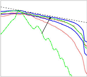
The results obtained from free-decay cases are presented in figure 1. Figure 1(a) shows the evolution of  $\varPsi _{in}/E_{in}$ with different nonlinearity levels, measured by the value of $\epsilon$ evaluated at $t=500T_p$. It can be seen that quasi-stationary states are established for all cases after $t=500T_p$. A typical spectral evolution for the case with $\epsilon =0.151$ is also shown as an inset to demonstrate the convergence of the spectrum to a power-law state. The spectra at quasi-stationary states for different nonlinearity levels (i.e. values of $\epsilon$) are shown in figure 1(b). At high nonlinearity level of $\epsilon =0.151$, we observe a clear power-law spectrum which has a slope $\alpha \approx -5/2$ consistent with WTT solution (1.1) in an approximate range of $[10,65]$. We note that the power-law range ends at $k\approx 65$ which is smaller than $k_d=115$, similar to other numerical simulations with a sharp dissipation cutoff (e.g. Dyachenko et al. Reference Dyachenko, Korotkevich and Zakharov2004; Pan & Yue Reference Pan and Yue2014), probably due to the interaction of the spectrum with the dissipation range that is not in a power-law form. With a decrease of nonlinearity level $\epsilon$, the power-law spectrum becomes shorter and steeper, reaching $\alpha \approx -3.4$ at $\epsilon =0.068$. This steepening of the spectra is in contrast to the results from Majda–McLaughlin–Tabak (MMT) turbulence with $\omega =k^2$ and quartet resonance (Hrabski & Pan Reference Hrabski and Pan2020), mainly because the latter forms a continuous resonant system (Faou, Germain & Hani Reference Faou, Germain and Hani2016) at low nonlinearity (we elaborate this more in § 3.4). We also remark that $\epsilon =0.151$ is about the highest nonlinearity we can reach in the current HOS context. The simulation for this strongly nonlinear case is possible using the HOS method because of the damping terms (2.3) and (2.4) which phenomenologically account for the wave breaking (e.g. Xiao et al. Reference Xiao, Liu, Wu and Yue2013). Previous free-decay simulations of Onorato et al. (Reference Onorato, Osborne, Serio, Resio, Pushkarev, Zakharov and Brandini2002) and Yokoyama (Reference Yokoyama2004) which result in $\alpha \approx -5/2$ are both conducted at a value of $\epsilon$ close to 0.15 (respectively 0.15 and 0.14).
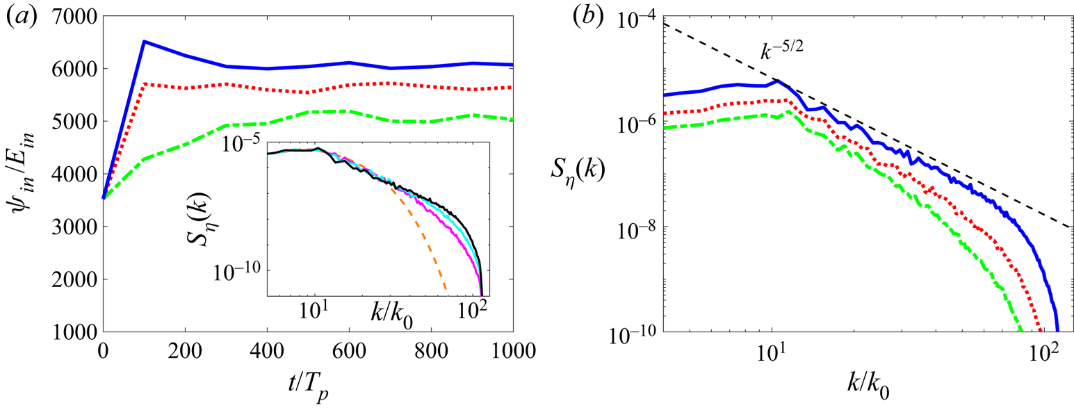
Figure 1. (a) Time evolution of  $\varPsi _{in}/E_{in}$ and (b) stationary spectra in free-decay cases with $\epsilon =0.068$ (- $\cdot$ -, green), $0.106$ ( $\boldsymbol {\cdot \ \cdot \ \cdot }$, red) and $0.151$ (—–, blue) evaluated at $t=500T_p$ from different runs. Inset of (a) shows wave spectra obtained at $t=0$ (– – –, orange), $100T_p$ (—–, magenta), $200T_p$ (—–, cyan) and $500T_p$ (—–) with $\epsilon =0.151$. The theoretical power-law scaling $k^{-5/2}$ (– – –) is indicated in (b) for reference.
The results from the forcing cases are shown in figure 2. The evolutions of  $\varPsi _{in}$ in the narrow-band and broad-band cases with different forcing amplitudes $f_0$ (resulting in different values of $\epsilon$ at the stationary state) are plotted in figures 2(a) and 2(c), all showing stationary states in $[1000T_p, 1500T_p]$. The stationary power-law spectra obtained at $t=1500T_p$ for the two cases are plotted in figures 2(b) and 2(d), respectively. For both cases, we observe that the spectral slopes $\alpha$ approach $-5/2$ at sufficiently high forcing/nonlinearity (consistent with previous work (Dyachenko et al. Reference Dyachenko, Korotkevich and Zakharov2004)). The power-law ranges for both cases begin immediately above $k=10$, even though the forcing is applied to the range above $k=10$. This is an indication that the nonlinear interaction is strong enough (relative to the forcing) to dominate the dynamics in this range. With a decrease of nonlinearity, the spectra for both cases become steeper, which are also reported in experiments in Falcon et al. (Reference Falcon, Laroche and Fauve2007), Nazarenko et al. (Reference Nazarenko, Lukaschuk, McLelland and Denissenko2010) and Deike et al. (Reference Deike, Miquel, Gutiérrez, Jamin, Semin, Berhanu, Falcon and Bonnefoy2015). However, we observe that the spectra at low nonlinearity clearly show a dependence on the bandwidth of the forcing, with the one from the narrow-band case much steeper (even not showing a power law) than the one from the broad-band case. It can also be noticed that, for the narrow-band case, the spectrum at low nonlinearity level ( $\epsilon =0.059$) exhibits discrete superharmonic peaks, are explained through bound waves in § 3.3.

Figure 2. (a) Time evolution of  $\varPsi _{in}$ and (b) stationary spectra obtained at $t=1500T_p$ in the broad-band forcing case with $f_0=3\times 10^{-7}$, $\epsilon =0.061$ (- $\cdot$ -, green); $f_0=1.6\times 10^{-6}$, $\epsilon =0.118$ ( $\boldsymbol {\cdot \ \cdot \ \cdot }$, red); $f_0=3.2\times 10^{-6}$, $\epsilon =0.145$ (—–, blue). (c) Time evolution of $\varPsi _{in}$ and (d) stationary spectra obtained at $t=1500T_p$ in the narrow-band forcing case with $f_0=8\times 10^{-7}$, $\epsilon =0.059$ (- $\cdot$ -, green); $f_0=4\times 10^{-6}$, $\epsilon =0.114$ ( $\boldsymbol {\cdot \ \cdot \ \cdot }$, red); $f_0=1\times 10^{-5}$, $\epsilon =0.148$ (—–, blue). The theoretical power-law scaling $k^{-5/2}$ (– – –) and boundaries of the forcing ranges (—–) are indicated in (b,d) for reference.
To obtain a complete view of spectral slopes for both the free-decay and forcing cases, we plot the values of  $\alpha$ in all cases as functions of the nonlinearity level in figure 3. This plot is limited above by the stability of the HOS method and below by the existence of a power-law spectrum. In practice, we consider a power-law spectrum not existing if the power-law range is less than 0.5 decade or if the spectrum is dominated by discrete peaks such as the one with low nonlinearity level in figure 2(d). We see that for all cases, the spectral slope $\alpha$ approaches the WTT value $-5/2$ at sufficiently high nonlinearity levels of $\epsilon \approx 0.15$. With a decrease of $\epsilon$, all spectra become steeper but with different steepening rates especially at relatively low nonlinearity level. It is also clear that the narrow-band forcing case shows a transition at $\epsilon _c \approx 0.11$, below which a very rapid steepening is observed. The mechanisms underlying these behaviours are further analysed in §§ 3.3 and 3.4.
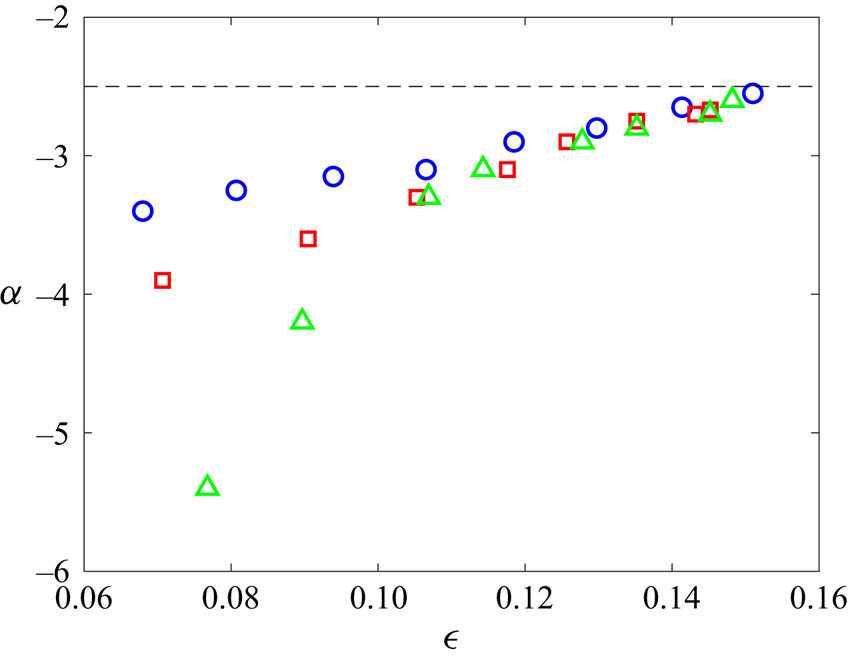
Figure 3. The spectral slope  $\alpha$ as functions of effective steepness $\epsilon$ for the free-decay ( $\circ$, blue), broad-band forcing ( $\Box$, red) and narrow-band forcing ( $\triangle$, green) cases, compared with the prediction of WTT with $\alpha =-5/2$ (– – –).
3.2. Energy flux
In this section, we investigate the scaling between the spectral level of  $S_\eta (k)$ and the energy flux $P$. For the evaluation of $P$, we can directly compute the energy transfer due to nonlinear terms in the primitive equation (Hrabski & Pan Reference Hrabski and Pan2020) or use energy dissipation rate as a measure of $P$ (e.g. Pan & Yue Reference Pan and Yue2014). For dissipation localized at high wavenumbers (such as our cases), the two approaches are equivalent (as all energy flux through the inertial range is dissipated at high wavenumbers in a stationary state). Therefore, we use dissipation rate as a measure of $P$, which takes the form (Pushkarev & Zakharov Reference Pushkarev and Zakharov1996; Pan & Yue Reference Pan and Yue2014)
 \begin{equation} P=\iint_{\boldsymbol{k}} \gamma_k(|\tilde{\eta}({\boldsymbol{k})}|^2+k|\widetilde{\phi^S}({\boldsymbol{k}})|^2)\,{\rm d}\boldsymbol{k}, \end{equation}
where  $\widetilde {\phi ^S}(\boldsymbol {k})$ is the spatial Fourier transform of $\phi ^S(\boldsymbol {x})$. We note that (3.5) is slightly less accurate in the free-decay case since the spectra slowly evolve in the quasi-stationary state. However, the evolution rate of the spectra is much smaller than the energy flux so that the associated error is negligible.
The scaling between  $E_{in}$ and $P^{1/3}$ is plotted in figure 4 for the free-decay case and the two forcing cases. The variable $P^{1/3}$ is used for the horizontal axis so that the WTT scaling $E_{in}\sim P^{1/3}$ becomes a straight line in the figure. We see that, at high nonlinearity level, the scaling in all cases approaches the WTT scaling, although the range of consistency is longer in the free-decay case and the broad-band forcing case. With the decrease of nonlinearity, the scaling deviates from the WTT prediction with a smaller value of $P$ for given $E_{in}$. This indicates a reduced capacity of energy cascade with the reduction of nonlinearity. As the nonlinearity level is further decreased, all curves approach states with $P\rightarrow 0$ and finite $E_{in}$, suggesting the formation of ‘frozen turbulence’, which is previously (only) introduced for capillary waves (Pushkarev & Zakharov Reference Pushkarev and Zakharov2000; Pan & Yue Reference Pan and Yue2014). This result is remarkable because of the existence of (sparse) exact resonances for gravity waves on a discrete grid of $\boldsymbol {k}$ (rational torus), in contrast to capillary waves. Before this study it is not clear whether the exact quartet resonances of gravity waves can be connected to result in a cascade (Kartashova, Nazarenko & Rudenko Reference Kartashova, Nazarenko and Rudenko2008), although this has been demonstrated to be possible in MMT turbulence (Hrabski & Pan Reference Hrabski and Pan2020). The results here suggest that the energy cascade should not be expected under the current wavenumber range in spite of the existence of energy transfer within a small number of resonant quartets. A more detailed study can be performed considering the kinematic expansions of exact quartet interactions (e.g. Lvov et al. Reference Lvov, Nazarenko and Pokorni2006; Hrabski et al. Reference Hrabski, Pan, Staffilani and Wilson2021).

Figure 4. Plots of the energy density in the inertial range  $E_{in}$ as a function of $P^{1/3}$ for free-decay ( $\circ$, blue), broad-band forcing ( $\Box$, red) and narrow-band forcing ( $\triangle$, green) cases, compared with the prediction of WTT $E_{in}\sim P^{1/3}$ (– – –).
In the following, we study hypothetical physical mechanisms concerning bound waves and the finite-size effect, which may lead to the spectral behaviours presented in §§ 3.1 and 3.2.
3.3. Bound waves
In this section, we study the effect of bound waves, which is argued as a major factor influencing spectral behaviour in previous experiments (Michel et al. Reference Michel, Semin, Cazaubiel, Haudin, Humbert, Lepot, Bonnefoy, Berhanu and Falcon2018). Here we generally define bound waves as wave components that do not satisfy the linear dispersion relation, no matter whether they are generated by carrier-wave distortion (Plant et al. Reference Plant, Keller, Hesany, Hara, Bock and Donelan1999, Reference Plant, Dahl, Giovanangeli and Branger2004), superharmonics (Herbert et al. Reference Herbert, Mordant and Falcon2010; Cobelli et al. Reference Cobelli, Przadka, Petitjeans, Lagubeau, Pagneux and Maurel2011; Michel et al. Reference Michel, Semin, Cazaubiel, Haudin, Humbert, Lepot, Bonnefoy, Berhanu and Falcon2018) or other mechanisms (Longuet-Higgins Reference Longuet-Higgins1992; Campagne et al. Reference Campagne, Hassaini, Redor, Valran, Viboud, Sommeria and Mordant2019) proposed in previous literature. In fact, as we show in § 3.3.1, all bound waves in a periodic-domain simulation can be interpreted through non-resonant nonlinear interactions. This definition distinguishes bound waves from free waves which satisfy the linear dispersion relation (or lie in its vicinity). To separate bound waves from the wave field, it is necessary to conduct a spatiotemporal analysis and obtain the wavenumber–frequency spectrum  $S_\eta (k,\omega )$, defined as
 \begin{equation} S_\eta(k,\omega)=\int_0^{2{\rm \pi}} |\tilde{\eta}(\boldsymbol{k},\omega)|^2 k \,{\rm d}\theta, \end{equation}
where  $\tilde {\eta }(\boldsymbol {k},\omega )$ is the spatiotemporal Fourier transform of $\eta (\boldsymbol {x},t)$:
 \begin{equation} \tilde{\eta}(\boldsymbol{k},\omega)=\iiint_{[0,T_L]\times[0,2{\rm \pi}]\times[0,2{\rm \pi}]} \eta(\boldsymbol{x},t)h_T(t)\exp({-{\rm i}(\boldsymbol{k}\boldsymbol{\cdot}\boldsymbol{x}-\omega t)})\,{\rm d}\boldsymbol{x}\,{\rm d} t, \end{equation}
with  $h_T(t)$ the Tukey window (Bloomfield Reference Bloomfield2004) of length $T_L=20T_p$, the time duration of the collected data within $1480T_p$– $1500T_p$ at the stationary state.
3.3.1. Generation mechanisms
The wavenumber–frequency spectra  $S_\eta (k,\omega )$ are plotted in figure 5 for narrow-band forcing with low and high nonlinearity levels, and broad-band forcing with low and high nonlinearity levels. The results for free-decay cases are not shown since they are somewhat similar to those for the broad-band forcing case. In all cases, we (seem to) observe significant amount of energy away from the linear dispersion relation (red curve in each panel), indicating the presence of bound waves in the simulations. In addition, the plot for narrow-band forcing at low nonlinearity (figure 5a) shows discrete peaks of bound-wave components, a visually distinct pattern from the other panels. With respect to the results in § 3.1, these discrete peaks correspond to the peaks in wavenumber spectra with low nonlinearity in figure 2(d). As marked by red dots in figure 5(a), these peaks can be quantified as superharmonics of the peak mode $(\omega _p, k_p)$ of carrier waves, in the form of
 \begin{equation} (\omega_b,k_b)=(n\omega_p,nk_p),\quad n=2,3,4,\ldots\end{equation}
The phase velocity for all bound-wave components, described by (3.8), can be computed as  $\omega _b/k_b=\omega _p/k_p$, which is the same as the phase velocity of the peak mode of carrier waves. Therefore, the bound waves can be considered as non-dispersive, i.e. they are ‘bound’ to the carrier wave as the latter travels. This behaviour agrees with some of the classical views of bound waves described in Lake & Yuen (Reference Lake and Yuen1978) and Plant (Reference Plant2003).

Figure 5. Normalized wavenumber–frequency spectra  $S_\eta (\omega,k)/S_\eta (\omega _p,k_p)$ in log scale for narrow-band forcing cases with (a) $\epsilon =0.059$ and (b) $\epsilon =0.148$ and for broad-band forcing cases with (c) $\epsilon =0.061$ and (d) $\epsilon =0.145$. The linear dispersion relation is marked by (—–, red). In (a), the peak modes are marked by ( $\bullet$, red) computed from (3.8) with $n= 2,3,4,5$. In (b–d), the lines corresponding to (3.9) with $m=2,3$ are indicated by $\boldsymbol {\cdot \ \cdot \ \cdot }$, and the lines corresponding to (3.10) with $l=-1,1,2$ are indicated by (– – –, brown).
For cases in figure 5(b–d), however, the bound-wave patterns are dramatically different from that in 5(a). It is clear from the plots that these bound-wave components are not necessarily non-dispersive, which is consistent with other general views of bound waves (e.g. Phillips Reference Phillips1981). In these cases, we observe several bound-wave branches (in contrast to the main branch of linear dispersion relation) on the spectra  $S_\eta (\omega,k)$. These bound-wave branches can be explained through two different mechanisms discussed below.
The first mechanism corresponds to the superharmonics of all free waves, i.e. modes  $(\omega,k)$ in the main (carrier) branch of the linear dispersion relation, satisfying
 \begin{equation} (\omega_b,k_b)=(m\omega,mk),\quad m=2,3,4,\ldots\end{equation}
The second mechanism corresponds to bound waves generated by the (non-resonant) interactions between the harmonics of peak mode  $(\omega _p,k_p)$ and an arbitrary free wave $(\omega,k)$ in the main branch, satisfying
 \begin{equation} (\omega_b,k_b)=(\omega+l\omega_p,k+lk_p),\quad l=\pm1,\pm2,\pm3,\ldots\end{equation}
 The curves described by (3.9) and (3.10) are marked in figure 5(b–d) respectively by black solid lines and brown dashed lines. The two mechanisms co-explain the superbranches of bound waves on the right of the main branch, as they both contribute to the energy in each of the visible superbranches. The second mechanism with  $l=-1$ further explains the sub-branches of bound waves on the left of the main branch. We remark that the two mechanisms (3.9) and (3.10) are also separately observed in experiments of Herbert et al. (Reference Herbert, Mordant and Falcon2010), Cobelli et al. (Reference Cobelli, Przadka, Petitjeans, Lagubeau, Pagneux and Maurel2011) and Campagne et al. (Reference Campagne, Hassaini, Redor, Valran, Viboud, Sommeria and Mordant2019). Our results here provide a more comprehensive view of bound waves: we need to consider the property of carrier waves to distinguish cases in figures 5(a) and 5(b–d), and consider combined mechanisms (3.9) and (3.10) for the explanation in the latter case.
3.3.2. Effects on wave spectra
Our next goal is to separate bound waves and free waves to elucidate their relative importance to the wave turbulence of gravity waves. The algorithm for the separation is illustrated in figure 6, which shows the definition of a free-wave finite band (by dashed line) in the vicinity of the linear dispersion relation. Specifically, this finite band is generated through a filter (similar to Campagne et al. Reference Campagne, Hassaini, Redor, Valran, Viboud, Sommeria and Mordant2019):
 \begin{equation}
f(\boldsymbol{k},\omega)\equiv\left\{\begin{array}{@{}lc} 1, &
|\omega-\omega_k| \leq \delta \omega, \\ 0, &
|\omega-\omega_k| > \delta \omega,
\end{array}\right.
\end{equation}
\begin{equation}
f(\boldsymbol{k},\omega)\equiv\left\{\begin{array}{@{}lc} 1, &
|\omega-\omega_k| \leq \delta \omega, \\ 0, &
|\omega-\omega_k| > \delta \omega,
\end{array}\right.
\end{equation}
where  $\delta \omega =0.6\omega _0$ is a parameter characterizing the width of the free-wave band, with $\omega _0=1$ the fundamental frequency in the domain. We have tested that this choice of $\delta \omega$ lies in a stationary range in terms of the results discussed below, i.e. reducing or increasing it results in respectively insufficient free-wave energy or contamination by bound-wave branches. For the separation, we apply the filter (3.11) directly to $\tilde {\eta }(\boldsymbol {k},\omega )$ and obtain the free-wave and bound-wave components as $\tilde {\eta }_f(\boldsymbol {k},\omega )=f(\boldsymbol {k},\omega )\tilde {\eta }(\boldsymbol {k},\omega )$ and $\tilde {\eta }_b(\boldsymbol {k},\omega )=\tilde {\eta }(\boldsymbol {k},\omega )-\tilde {\eta }_f(\boldsymbol {k},\omega )$. Then we compute the free-wave spectra $S_{\eta }^f(k,\omega )$, $S_{\eta }^f(k)$ and bound-wave spectra $S_{\eta }^b(k,\omega )$, $S_{\eta }^b(k)$ likewise using (3.6) and (3.1). We note that it is also possible to directly apply the filter (3.11) to $S_\eta (k,\omega )$ for the separation, but our operation (with respect to $\tilde {\eta }$) is desirable due to the study that is discussed in § 3.4.
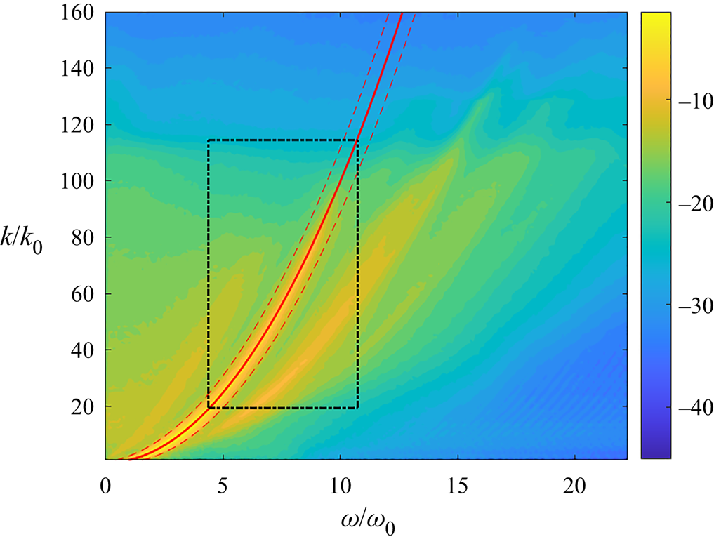
Figure 6. A typical illustration for the separation of free and bound waves in a wavenumber–frequency spectrum. The region of  $[\omega _k-\delta \omega,\omega _k+\delta \omega ]$ defined in (3.11) is marked by (– – –, red). The region bounded by - $\cdot$ - corresponds to the inertial ranges $[\omega _c,\omega _d]\times [k_c,k_d]$ used in (3.12).
The free-wave and bound-wave wavenumber spectra are shown in figure 7 for all three (free-decay and broad-band and narrow-band forcing) cases at high and low nonlinearity levels. In most cases, we find that the power-law ranges of the spectra are dominated by free-wave components with their energy at least one order of magnitude higher than those of the bound-wave components. The only exception is the case with narrow-band forcing at low nonlinearity level shown in figure 7(e), where bound waves dominate most of the range above  $k\approx 17$ exhibiting discrete peaks. On the other hand, waves at sufficiently small scales in the dissipation range are dominated by bound waves in all cases, but their influences to the inertial-range spectra are not significant.
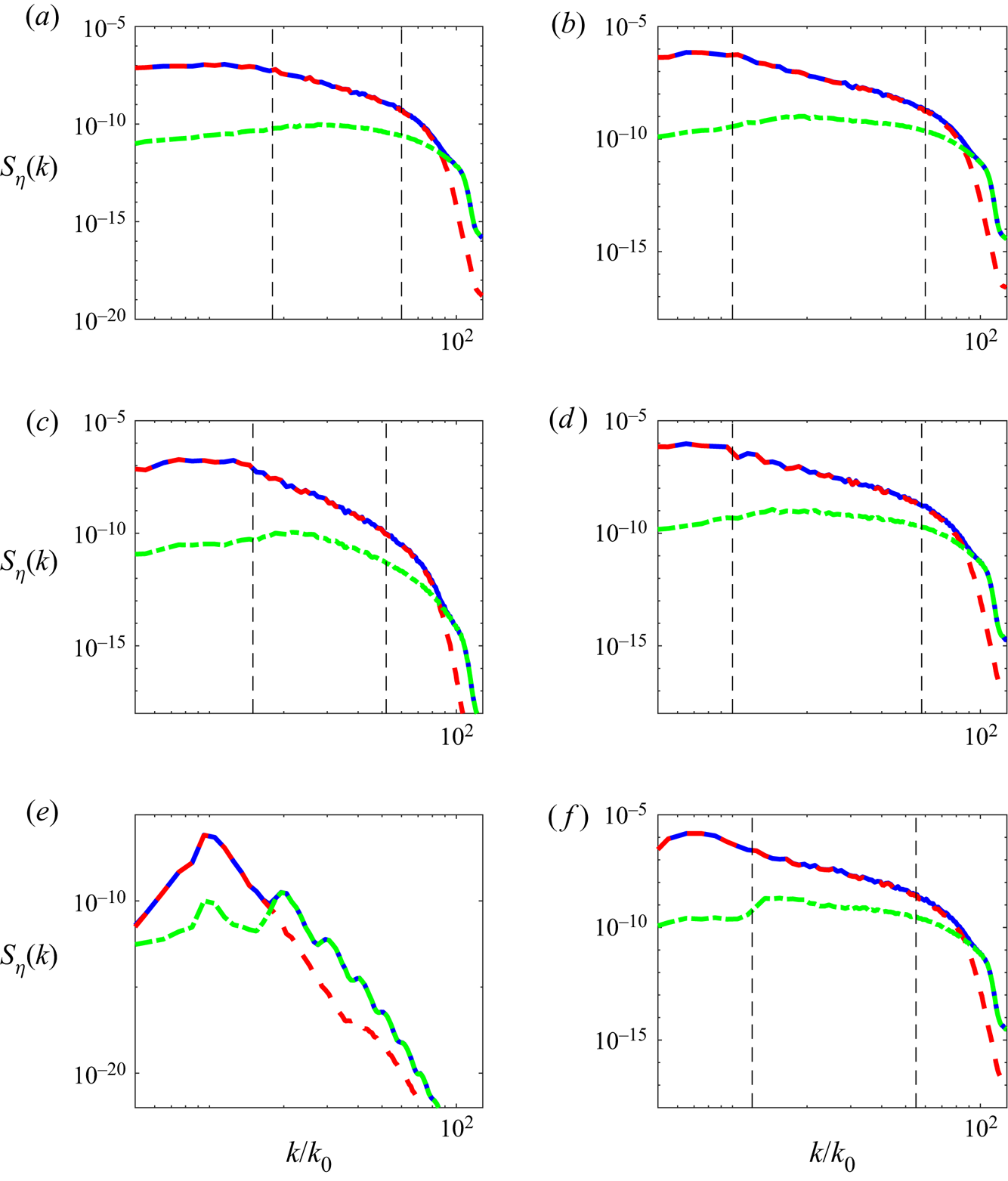
Figure 7. Plots of  $S_\eta ^f(k)$ (– – –, red), $S_\eta ^b(k)$ (- $\cdot$ -, green) and $S_\eta (k)$ (—–, blue) in free-decay cases with (a) $\epsilon =0.068$ and (b) $\epsilon =0.151$; broad-band forcing cases with (c) $\epsilon =0.071$ and (d) $\epsilon =0.145$; narrow-band forcing cases with (e) $\epsilon =0.059$ and (f) $\epsilon =0.148$. The boundaries of the power-law ranges are indicated by – – –, except for (e) where discrete peaks are observed.
The general behaviour of bound waves in figure 7 suggests that they are not the major factor causing the steepening of the spectra except in the narrow-band forcing case. This point will be made more clear after further quantifying the fraction of bound waves in the wave field. For this purpose, we define the bound-wave energy in the inertial range as
 \begin{equation} E_b\equiv\int_{\omega_c}^{\omega_d}\int_{k_c}^{k_d} S_{\eta}^b(k,\omega)\,{\rm d} k\,{\rm d}\omega, \end{equation}
where  $[k_c, k_d]$ and $[\omega _c=k_c^{1/2}, \omega _d=k_d^{1/2}]$ are a box describing the limits of inertial range as shown in figure 6. We quantify the fraction of bound waves using the ratio of $E_b/E_t$, where $E_t$ is the total wave energy in the inertial range computed in a similar way to (3.12) but with $S_{\eta }(k,\omega )$ replacing $S_{\eta }^b(k,\omega )$.
Figure 8 summarizes the quantity  $E_b/E_t$ at different nonlinearity levels for all three cases. For the broad-band forcing and free-decay cases, we see that the fraction of bound-wave energy consistently decreases with a decrease of nonlinearity level. This provides a clear evidence that the steepening of the spectra with the decrease of nonlinearity is not caused by bound waves in these cases. For the narrow-band forcing case, the fraction of bound-wave energy is consistently larger than those in the other two cases (at all nonlinearity levels). In addition, with a decrease of nonlinearity, a transition occurs at a critical nonlinearity level ( $\epsilon _c\approx 0.11$), below which $E_b/E_t$ increases with a decrease of $\epsilon$. In general, we expect the critical level $\epsilon _c$ to increase with a decrease of the forcing bandwidth. (For the broad-band forcing case considered here, the frozen turbulence regime is reached first with a decrease of nonlinearity, so $\epsilon _c$ does not exist in this case.) The critical level $\epsilon _c$ is consistent with the transition in figure 3, below which a much more rapid steepening of the spectral slope is observed for the narrow-band forcing case. We thus conclude that the presence of bound waves explains the largest steepening rate of the spectra at low nonlinearity levels in the narrow-band forcing case. Moreover, the significant fraction of bound waves in the narrow-band forcing case also provides an explanation of the rapid deviation from $E_{in}\sim P^{1/3}$ shown in figure 4, since bound waves account for energy which does not follow the WTT cascade pathway.
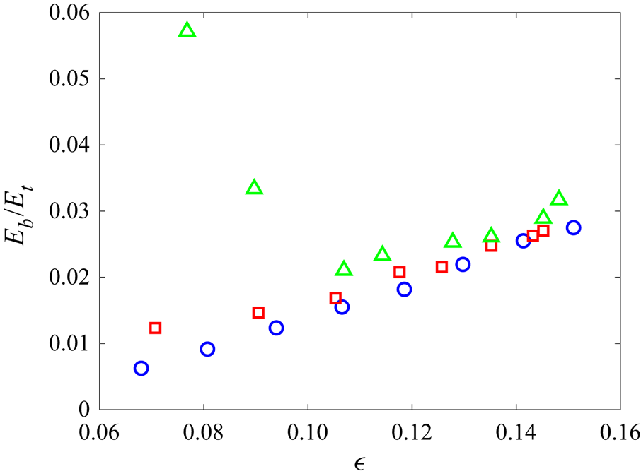
Figure 8. The proportions of bound-wave energy  $E_b/E_t$ as functions of $\epsilon$ for the free-decay ( $\circ$, blue), broad-band forcing ( $\Box$, red) and narrow-band forcing ( $\triangle$, green) cases.
We finally remark that while the transition at  $\epsilon _c$ in figure 8 is consistent with the transition to rapid variation of $\alpha$ in figure 3, the percentage of bound waves remains not significant for the range of nonlinearity levels considered in the two figures. As a result, computing the spectral slope from $S_\eta ^f(k)$ provides almost the same values as those shown in 3, as evidenced from figure 7 for many cases (which is also true for the narrow-band forcing cases at nonlinearity levels associated with power-law spectra). Physically, this suggests that bound waves cannot be simply considered as linear superpositions on free waves. Instead, their nonlinear interactions with free waves can be important in understanding the evolution and dynamics of the wave fields.
3.4. Finite-size effect
In order to further understand the steepening of spectra and reduced energy flux capacity at low nonlinearity levels, we investigate another hypothetical mechanism of the finite-size effect. In general, the finite-size effect arises due to the violation of the assumption of the infinite domain in WTT (Pushkarev & Zakharov Reference Pushkarev and Zakharov2000; Lvov et al. Reference Lvov, Nazarenko and Pokorni2006; Nazarenko Reference Nazarenko2006). In the framework of the WTT kinetic equation, the energy cascade is enabled by modes on the continuous resonant manifold satisfying (for gravity waves)
 $$\begin{gather} \boldsymbol{k}_1+\boldsymbol{k}_2=\boldsymbol{k}_3+\boldsymbol{k}, \end{gather}$$
 $$\begin{gather}\omega_1+\omega_2=\omega_3+\omega, \end{gather}$$
where  $\omega _i^2=k_i$ ( $i=1,2,3$). In a finite domain, discreteness of wavenumber and frequency (imposed by the domain boundary) reduces the manifold defined by (3.13) and (3.14) by limiting the resonances to discrete points. This discreteness effect can be compensated by the nonlinear broadening which allows the occurrence of quasi-resonances, characterized by a modification of (3.14) as
 \begin{equation} |\omega_1+\omega_2-\omega_3-\omega|<\varDelta \omega, \end{equation}
with  $\varDelta \omega$ a nonlinear broadening parameter depending on the nonlinearity level.
One way to quantify the finite-size effect (in particular to measure the nonlinear broadening and interaction strength) of gravity waves is through a tri-coherence analysis (see e.g. Pan & Yue (Reference Pan and Yue2017) for a bi-coherence study of capillary waves). We first define a tri-coherence function
 \begin{equation} T(\boldsymbol{k},\boldsymbol{k}_1,\boldsymbol{k}_2)\equiv\frac{|\langle\tilde{\eta}_f(\boldsymbol{k}_1,t) \tilde{\eta}_f(\boldsymbol{k}_2,t)\tilde{\eta}_f^*(\boldsymbol{k}_3,t)\tilde{\eta}_f^*(\boldsymbol{k},t)\rangle|}{\langle| \tilde{\eta}_f(\boldsymbol{k}_1,t)||\tilde{\eta}_f(\boldsymbol{k}_2,t)||\tilde{\eta}_f^*(\boldsymbol{k}_3,t)|| \tilde{\eta}_f^*(\boldsymbol{k},t)|\rangle}, \end{equation}
where  $\boldsymbol {k}_3 \equiv -\boldsymbol {k}+\boldsymbol {k}_1+\boldsymbol {k}_2$, $\langle \cdot \rangle$ denotes the time average (for stationary states) and an asterisk denotes the complex conjugate. Here $\tilde {\eta }_f(\boldsymbol {k},t)$ corresponds to the free-wave modes, and is computed by the spatial Fourier transform of $\eta _f(\boldsymbol {x},t)$ with the latter obtained after applying the filter (3.11) to the wavenumber–frequency spectra. By definition, the function $T(\boldsymbol {k},\boldsymbol {k}_1,\boldsymbol {k}_2)$ continuously varies between 0 and 1. In particular, $T$ takes larger values for quartets closer to exact resonance, with the maximum value of 1 achieved for exact resonances among $\boldsymbol {k}$, $\boldsymbol {k}_1$, $\boldsymbol {k}_2$ and $\boldsymbol {k}_3$ satisfying (3.14). In (3.16), we use $\tilde {\eta }_f$ instead of $\tilde {\eta }$ for the evaluation to remove the contamination by bound waves since they result in noisy values of $T$ not lying in the vicinity of the resonant manifold (as found in previous work (Pan & Yue Reference Pan and Yue2017)). This operation is also compatible with findings in § 3.3 that bound waves do not contribute to the general steepening of the spectra (except in the narrow-band forcing case).
To facilitate the visualization of  $T$, we fix $\boldsymbol {k}_1=(40,40)$ and $\boldsymbol {k}_2=(20,-40)$ so that $T(\boldsymbol {k})$ with $\boldsymbol {k}=(k_x,k_y)$ can be shown by two-dimensional contour plots. Figure 9 shows such plots of $T(\boldsymbol {k})$ in the broad-band forcing case at three different nonlinearity levels. The results for the narrow-band forcing and free-decay cases are not included due to their similarity to the presented results (the quantification of broadening and interaction strength for all cases is presented later). Also shown in figure 9 is the continuous resonant manifold (red lines) satisfying (3.13) and (3.14), and the discrete resonant points (red crosses) with $\boldsymbol {k}$ only taking integer values. In particular, to compute the resonant manifold we need to consider the wave travelling direction and the complex conjugate relation for real functions, with details presented in Appendix A.

Figure 9. The tri-coherence  $T(\boldsymbol {k},\boldsymbol {k}_1,\boldsymbol {k}_2)$ with $\boldsymbol {k}_1=(40,40)$, $\boldsymbol {k}_2=(20,-40)$ for broad-band forcing cases with (a) $\epsilon =0.071$, (b) $\epsilon =0.118$ and (c) $\epsilon =0.145$. The continuous resonant manifold is plotted by (—–, red). The discrete resonant solutions with $\boldsymbol {k}\in (\mathbb {Z},\mathbb {Z})$ are marked by ( $\times$, red). The data for generating these figures are collected from $t=1460T_p$ to $t=1500T_p$ in the stationary state. (d–f) Zoom-in views of (a–c) respectively.
From figure 9(a–c) we can see that all significant values of  $T$ are concentrated close to the resonant manifold (as a result of using $\tilde {\eta }_f$ in (3.16)). It is also clear that the nonlinear broadening is visibly wider at a higher nonlinearity level compared with that at a lower nonlinearity level. The finite-size effect can be further visualized through the zoom-in views in figure 9(d–f). At low nonlinearity, figure 9(d) shows discrete peaks of $T\sim O(1)$ at only a number of grid points $(k_x,k_y)$ lying on or very close to the resonant manifold. This is a direct result of the finite-size effect, as it is in contrast to the situation of $T$ taking uniform values of 1 on the resonant manifold that can be expected in an infinite domain. With an increase of nonlinearity level from figure 9(d) to 9(f), the broadening of the interaction width overcomes the discreteness in $T$, alleviating its destructing effect on the nonlinear interactions.
In addition, the discrete resonant points seem to be sparse on the continuous manifold, with all four points in each panel of figure 9 as trivial quartet solutions (either with repetition or symmetry with given vectors of  $\boldsymbol {k}_1$ and $\boldsymbol {k}_2$). This sparsity can be further demonstrated by a numerical analysis which identifies no non-trivial solution with stretching of the current resonant manifold (see Appendix B). This problem has also been considered analytically and numerically in Kartashova (Reference Kartashova2006) and Lvov et al. (Reference Lvov, Nazarenko and Pokorni2006), which reach a consistent conclusion on the rareness of the discrete solutions except for two special types of collinear quartets and tridents (which, however, do not exist in our case with waves propagating only to the positive $x$ direction). Moreover, the sparsity of discrete solutions in this case is in contrast to the situation of the $\omega =k^2$ MMT dispersion relation studied in Hrabski & Pan (Reference Hrabski and Pan2020). The difference in the structure of the discrete resonant solutions is the key for the gravity-wave spectra and MMT spectra to show completely different behaviours at low nonlinearity, with the former deviating from the WTT spectral slope but the latter approaching the WTT spectral slope.
To further quantify the effect of nonlinearity level on quartet resonances, we define two measures  $\hat {L}_b$ and $I$ respectively for the broadening width and overall interaction strength. For $\hat {L}_b$, we define it as a characteristic width (Pan & Yue Reference Pan and Yue2017):
 \begin{equation} \hat{L}_b\equiv\frac{\sum_{\boldsymbol{k}} |\hat{\varOmega}|T(\boldsymbol{k})}{\sum_{\boldsymbol{k}} T(\boldsymbol{k})}, \end{equation}
where  $|\hat {\varOmega }|$ is the normalized frequency mismatch given by $|\hat {\varOmega }|=|\varOmega |/k^{-1/2}$ with $\varOmega \equiv \omega _1+\omega _2-\omega _3-\omega _k$ and the denominator $k^{-1/2}$ estimating the frequency discreteness at $k$ associated with the wavenumber spacing. In (3.17), the summation is for all the grid points of $\boldsymbol {k}$. Thus, $\hat {L}_b$ measures the nonlinear broadening around the exact solutions by the first moment of $T(\boldsymbol {k})$.
We further define  $I$ as
 \begin{equation} I\equiv\sum_{\boldsymbol{k}} T(\boldsymbol{k}), \end{equation}
which measures the overall interaction strength by summing up contributions from both resonant and quasi-resonant interactions. We remark that  $I$ provides supplemental information to $L_b$, because $L_b$ itself does not quantify the dynamics of energy transfer, i.e. a larger $L_b$ does not mean a stronger energy transfer if the function $T$ becomes more discrete in the interaction broadening region. In contrast, $I$ provides a measure of the overall interaction strength accounting for both the finite-size effect and the nonlinear broadening. Another improved quantification of the interaction strength of exact and quasi-resonances through a quartet-level decomposition of the energy flux can be found in Hrabski & Pan (Reference Hrabski and Pan2021).
The characteristic width  $\hat {L}_b$ and the interaction strength $I$ are plotted as functions of $\epsilon$ for all cases in figure 10. We can observe a general increase of $\hat {L}_b$ and $I$ for increasing $\epsilon$, indicating a wider nonlinear broadening and a larger interaction strength with more quasi-resonances alleviating the finite-size effect. We remark that this clear behaviour of $\hat {L}_b$ and $I$ is only possible to resolve by using $\tilde {\eta }_f$ to evaluate the tri-coherence. The general trend of $\hat {L}_b$ with respect to $\epsilon$ seems to be consistent with the nonlinear detuning (or correction) of the dispersion relation introduced in Stuhlmeier & Stiassnie (Reference Stuhlmeier and Stiassnie2019), but the exact relation between the two quantities is yet to be understood. The reduction of the nonlinear broadening and the interaction strength with decreasing nonlinearity is consistent with the steepening of spectra and the reduction of energy flux capacity discussed in §§ 3.1 and 3.2. Therefore, we conclude that the finite-size effect is a major contributor to the spectral behaviours at low nonlinearity levels (especially for cases with sufficient spectral bandwidth). Finally, the values of $\hat {L}_b$ and $I$ in the narrow-band forcing case are slightly smaller than in the other two cases for all nonlinearity levels, probably because of the higher fraction of bound waves (which leads to a larger $\epsilon$ than the other two cases, but not larger $\hat {L}_b$ or $I$).
$I$).

Figure 10. (a) The characteristic length of nonlinear broadening  $\hat {L}_b$ and (b) the intensity of nonlinear interactions $I$ as functions of $\epsilon$ for the free-decay ( $\circ$, blue), broad-band forcing ( $\Box$, red) and narrow-band forcing ( $\triangle$, green) cases.
4. Conclusions
We conduct numerical simulation of Euler equations to study the surface gravity wave turbulence in three representative conditions, namely free-decay, narrow-band forcing and broad-band forcing turbulence. In all cases, We find that the scalings of the wave spectra with wavenumber and energy flux both approach the WTT solution at sufficiently high nonlinearity levels. With a decrease of nonlinearity level, steeper spectra and reduced energy flux capacity can be observed indicating the deviation from WTT, with the largest deviation rate found in the narrow-band forcing case. Two hypothetical mechanisms for bound waves and finite-size effect to explain these spectral variations are investigated. For bound waves, we elucidate their generation mechanisms through a spatiotemporal analysis (which generalizes the previous study of this topic) and find that their fraction generally decreases with a decrease of nonlinearity level except for the narrow-band forcing case. This suggests that bound waves only account for the rapid deviation from WTT in the narrow-band forcing case (but not for the other two cases). For the finite-size effect, we perform a tri-coherence analysis and find that both the nonlinear broadening and interaction strength decrease with a decrease of nonlinearity level, which accounts for the deviation from WTT at low nonlinearity levels in all cases of our simulation. We finally remark that cautions have to be taken in applying these numerical findings to experiments due to the additional complexity inevitably involved in the latter.
Declaration of interests
The authors report no conflict of interest.
Appendix A. Computation of resonant manifold in figure 9
We start by considering a (quasi-)stationary wave field described by
 \begin{equation} \eta(\boldsymbol{x},t) = \sum_i A_i \exp({{\rm i}(\boldsymbol{\kappa}_i \boldsymbol{\cdot} \boldsymbol{x} -\omega_i t )}) + A_i^* \exp({-{\rm i}(\boldsymbol{\kappa}_i \boldsymbol{\cdot} \boldsymbol{x} -\omega_i t )}),\end{equation}
where  $A_i=|A_i|\,{\rm e}^{{\rm i}\phi _i} \in \mathbb {C}$ and $\omega _i \in \mathbb {R}^+$. Since the wave fields in our simulations generally only contain waves travelling to the positive $x$ direction (due to the setting of initial condition and forcing), for each mode in (A1) we have $\kappa _{ix}\cdot \omega _i>0$ so that $\boldsymbol {\kappa }_i=(\kappa _{ix},\kappa _{iy})\in (\mathbb {R}^+,\mathbb {R})$.
Considering  $\tilde {\eta }(\boldsymbol {k},t)$ with $\boldsymbol {k}\in (\mathbb {R},\mathbb {R})$ as the spatial Fourier transform of $\eta (\boldsymbol {x},t)$, we can see that
 \begin{equation}
\tilde{\eta}(\boldsymbol{k}_i,t)=\left\{\begin{array}{@{}lc}
A_i \,{\rm e}^{-{\rm i} \omega_i t }, & k_{ix} > 0,
\\ A_i^* \,{\rm e}^{{\rm i}\omega_i t }, & k_{ix}
< 0.
\end{array}\right.
\end{equation}
\begin{equation}
\tilde{\eta}(\boldsymbol{k}_i,t)=\left\{\begin{array}{@{}lc}
A_i \,{\rm e}^{-{\rm i} \omega_i t }, & k_{ix} > 0,
\\ A_i^* \,{\rm e}^{{\rm i}\omega_i t }, & k_{ix}
< 0.
\end{array}\right.
\end{equation}
Substituting (A2) into (3.16), we obtain
 \begin{equation} T=|\langle \exp({{\rm i}(-\varOmega_d t + \varPhi_d)}) \rangle|, \end{equation}
where  $\varPhi _d=\phi _1+\phi _2-\phi _3-\phi$ and
 \begin{equation} \varOmega_d={\rm sgn}(k_{1x}) \omega_1+{\rm sgn}(k_{2x})\omega_2-{\rm sgn}(k_{3x})\omega_3-{\rm sgn}(k_x)\omega, \end{equation}
with
 \begin{equation} {\rm
sgn}(x)=\left\{\begin{array}{@{}lc} 1, & x > 0, \\
-1, & x < 0. \end{array}\right.
\end{equation}
\begin{equation} {\rm
sgn}(x)=\left\{\begin{array}{@{}lc} 1, & x > 0, \\
-1, & x < 0. \end{array}\right.
\end{equation}
In our case, we have  $k_{1x}=40>0$, $k_{2x}=20>0$ and $k_{3x}=k_{1x}+k_{2x}-k_x=60-k_x$, so that (A4) is reduced to $\varOmega _d=\omega _1+\omega _2-{\rm sgn}(60-k_x)\omega _3-{\rm sgn}(k_x)\omega$. We are interested in the case of $\varOmega _d=0$, which results in $T=1$ indicating the resonant manifold. Whether $\varOmega _d=0$ can be realized needs to be discussed in the following three situations (summarized in figure 11a):
(i) For $k_x<0$, we need $\varOmega _d=\omega _1+\omega _2-\omega _3+\omega =0$ which has no solution (for $\omega \in \mathbb {R}^+$) on the $(k_x,k_y)$ plane.
(ii) For
$0< k_x<60$, we need $\varOmega _d=\omega _1+\omega _2-\omega _3-\omega =0$ which has solutions shown as an ellipse bounded by $k_x=0$ and $k_x=60$ in figure 11(b). These solutions correspond to the resonant manifold shown in figure 9.(iii) For
$k_x>60$, we have $\varOmega _d=\omega _1+\omega _2+\omega _3-\omega =0$ which has no solution on the $(k_x,k_y)$ plane.


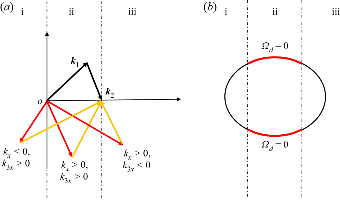
Figure 11. (a) Sketches of the three situations under discussion. Vectors  $\boldsymbol {k}_1$ and $\boldsymbol {k}_2$ are indicated in the figure; $\boldsymbol {k}$ and $\boldsymbol {k}_3$ are denoted by red and yellow arrows. The two vertical lines mark the boundaries of situations (i), (ii) and (iii) in the discussion. (b) The solution in situation (ii) as denoted by red lines (ellipse bounded by the two vertical lines).
In summary, the resonant manifold shown in figure 9 corresponds to the second case above, which is the only possibility to have solutions in  $\varOmega _d=0$ for a wave field travelling to the positive $x$ direction.
Appendix B. Sparsity of the discrete resonant solutions
We count the number of discrete resonant solutions as in figure 9, but with stretched  $\boldsymbol {k}_1$ and $\boldsymbol {k}_2$. The purpose is to demonstrate the sparsity of discrete resonances with the expansion of the resonant manifold. In particular, we define $\boldsymbol {k}_1=\lambda (40,40)$ and $\boldsymbol {k}_2=\lambda (20,-40)$, where $\lambda$ is a factor of stretching, and compute the number of exact resonances $N$ as a function of $\lambda$. For $\lambda$ varying from 1 to 10, our numerical searching algorithm gives $N=4$ always, indicating that no non-trivial solution can be identified. While this numerical study is presented for $\boldsymbol {k}_1$ and $\boldsymbol {k}_2$ in particular directions, we have also tested other directions to confirm that the exact resonances are indeed sparse for gravity waves.


 Open access