1 Introduction
Models describing the propagation and evolution of nonlinear surface gravity waves in the ocean are an indispensable tool for the coastal and ocean engineering and science communities. Among these, models for a regime in which the wavelength  $\unicode[STIX]{x1D706}$ is large compared to water depth $h$ are applicable in a wide range of settings, covering the behaviour of swell, wind waves and infragravity waves in the nearshore ocean to tsunami waves propagating at ocean basin scales. Waves falling in this regime $h/\unicode[STIX]{x1D706}\ll 1$ are weakly dispersive, having phase speeds that differ only slightly from the long-wave speed $c_{0}=\sqrt{gh}$.
In order to organize discussion, we write the dispersion relation for linear waves as
where $c$ is phase speed, $\unicode[STIX]{x1D714}=2\unicode[STIX]{x03C0}/T$ is angular frequency and $k=2\unicode[STIX]{x03C0}/\unicode[STIX]{x1D706}$ is wavenumber. For finite depths ($kh=O(1)$), $P(kh)=\tanh (kh)/kh$. In the limit as $kh\rightarrow 0$, $P(kh)\rightarrow 1$ and the appropriate model is given by the nonlinear long-wave equations, which neglect all effects of frequency dispersion. For waves where $kh$ is not vanishingly small, use of power series representations of the vertical structure of dependent variables typically leads to approximations of $P(kh)$ in the form of rational polynomials involving truncated series in powers of $(kh)^{2}$. Models of this type are collectively referred to here as Boussinesq-type equations (BTEs) if they correspond to a regime where both dispersion and nonlinearity are weak and do not appear in a combined fashion in the equations, and Serre or fully nonlinear Boussinesq-type equations (FNBTEs) if no limitation is imposed on the size of nonlinearity, characterized by the ratio of wave amplitude to water depth. (For more comprehensive overviews, see e.g. Brocchini (Reference Brocchini2013) and Kirby (Reference Kirby2016).)
The question of the stability of wave solutions is central to the analysis of both physical waves and the underlying models leading to their description. Nonlinear waves have a number of unstable behaviours, including long-wave or sideband instabilities and various sub- and superharmonic instabilities leading to behaviours such as cuspate perturbations of wave crests. These instabilities involve interactions between components with frequencies or wavenumbers that are not drastically different from each other, and generally involve a conservative transfer of energy between the involved components. In contrast, the approximations embedded in BTE or FNBTE models can lead to non-physical instabilities that are intrinsic to the model rather than to the waves being described. The question of linear stability is well understood. Referring to (1.1), it is clear that $P<0$ would lead immediately to unstable behaviour with $\unicode[STIX]{x1D714}$ imaginary. The possibility of this occurring can be seen by examining several asymptotically equivalent forms
where each approximation is equivalent to within errors of $O(kh)^{4}$. Clearly, a model that embodies the second approximation is linearly stable, whereas a model in the first form would be unstable for values of $kh>\sqrt{3}$, which is not a terribly useful range in a highly resolved model with a large cutoff wavenumber. These instabilities are typically short relative to the underlying wave being simulated, and impose restrictions on the choice of BTE or FNBTE approximation to use.
2 Overview
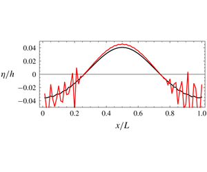
Recently, Madsen & Fuhrman (Reference Madsen and Fuhrman2020, MF20) have uncovered a comparable short-wave instability that arises from the nonlinear components of dispersive terms in FNBTE models. The instability is present in a number of long-accepted, linearly stable models. The mechanism is limited to the FNBTE class of models and does not affect the weakly nonlinear, weakly dispersive BTE models. The instability, which is concentrated in the trough region of the wave (where the surface is suppressed below the mean water level), can lead to the rapid growth of perturbations and destroy the underlying solution, as illustrated in the figure by the title (provided by Madsen & Fuhrman, where black and red lines show results of a sample calculation with an unstable model after 89 and 95 time steps).
The nonlinear instability mechanism is revealed using a perturbation approach. An initial solution to the FNBTEs is assumed and then perturbed, and linearized equations for the behaviour of the perturbation are isolated. Taking advantage of extensive experience with numerical solutions of the equations, MF20 assume that the unstable perturbation will have a short wavelength (or high $kh$) relative to the underlying long wave, and will be concentrated in the slowly varying wave trough. The analysis is then further simplified by neglecting derivatives of the underlying wave-induced flow in the trough region, reducing it to a steady flow with a shifted mean water level. The resulting dispersion relation for the perturbation is affected by a wave-current-like frequency shift, a shift in the apparent mean water depth, and corresponding shifts in the structure of the rational polynomial $P$ in (1.1). The resulting changes in the structure of $P$ reintroduce the possibility of having instability, not of the underlying solution, but of short perturbations to the underlying solution. MF20 analyse a number of FNBTE models, ranging from a typical $O(kh)^{2}$ approximation commonly found in practical applications (Wei et al. Reference Wei, Kirby, Grilli and Subramanya1995; Shi et al. Reference Shi, Kirby, Harris, Geiman and Grilli2012) to the much higher-order approximations of Madsen, Bingham & Lu (Reference Madsen, Bingham and Lu2002) and Liu, Fang & Cheng (Reference Liu, Fang and Cheng2018), each of which provides accurate access to water depths extending far into the deep-water range. MF20 find that each of these models is affected by instability in at least some range of conditions, with the minimum $kh$ for the onset of instability pushed to larger and larger values as model accuracy increases. Nevertheless, a general conclusion is reached that all FNBTE models are affected to some degree.
MF20 offer several suggestions for suppressing the instability. First, the high-order approximations used in their own group utilize the canonical surface boundary conditions due to Zakharov (Reference Zakharov1968), as also used in the class of high-order spectral (HOS) models (e.g. Dommermuth & Yue Reference Dommermuth and Yue1987). Noting that HOS models, which employ the full dispersion relation (1.1) for each spectral component, do not exhibit comparable trough instabilities, they suggest that a correct representation of frequency dispersion across all component frequencies could be crucial to suppressing the instability. This correction would be manifested through a correct treatment of the relation between component amplitudes $u_{n}$ for horizontal velocities and $w_{n}$ for vertical velocities, which, in linear theory, are related at the mean water level by $w_{n}/u_{n}=\tanh kh$, but with $\tanh kh$ again truncated in different ways in each FNBTE model. Sample calculations are mentioned in which the correct linear connection formula is used to determine $w_{n}$ from $u_{n}$, leading to solutions that do not exhibit instability. Alternatively, a rearrangement of reference levels for the definition of Taylor series for the vertical structure of dependent variables in the higher-order models also is seen to allow for a significant reduction in the extent of the unstable parameter space.
3 Future
The instability mechanism discovered by MF20 presents a significant challenge for the operation of accurate, energy-conserving models of Boussinesq type. Since the lower-order models of the type introduced by Serre (Reference Serre1953) or Wei et al. (Reference Wei, Kirby, Grilli and Subramanya1995), among others, are in extensive use in engineering and scientific practice, it will be of interest to examine the consequences of the stability analysis across a broader range of existing models. Following the analysis procedure presented in MF20, we find that the model equations of Serre (Reference Serre1953) (see also Su & Gardner (Reference Su and Gardner1969)), as well as the extension of the weakly nonlinear Boussinesq model of Peregrine (Reference Peregrine1966) to fully nonlinear form (not shown here), do not appear to be subject to the same trough instability as the model of Wei et al. (Reference Wei, Kirby, Grilli and Subramanya1995) or other models cited by Madsen & Fuhrman (Reference Madsen and Fuhrman2020) in their § 7. This writer initially thought that this may be tied to the use of depth-averaged horizontal velocity as the dependent variable and the resulting simplification of the equation for volume conservation, but the model of Madsen & Schäffer (Reference Madsen and Schäffer1998) is in this form and is unstable, and thus the explanation for this result is not yet clear.
Although the connection is not yet well established, it is possible that the instability identified by MF20 could contribute to the growth of noise seen in early finite-difference solutions of FNBTEs, which was not well described in the literature and was often suppressed using numerical filters. This early experience contributed to the modelling community’s shift to a preference for finite-volume total variation diminishing schemes around a decade ago (see e.g. Tonelli & Petti Reference Tonelli and Petti2009; Roeber, Cheung & Kobayashi Reference Roeber, Cheung and Kobayashi2010; Shi et al. Reference Shi, Kirby, Harris, Geiman and Grilli2012). These schemes apparently provide enough artificial numerical dissipation to mask the growth of trough instabilities, and thus allow for extremely long simulation times over domains with appreciable depth irregularities. However, this stability comes at the cost of wave damping, which is prohibitively large for cases where highly accurate results are needed or propagation over long distances is involved. Methods for deriving model equations that are not subject to potential trough instabilities will be needed if the modelling community is to be able to return to the use of less artificially dissipative schemes.


1 Introduction
Models describing the propagation and evolution of nonlinear surface gravity waves in the ocean are an indispensable tool for the coastal and ocean engineering and science communities. Among these, models for a regime in which the wavelength $\unicode[STIX]{x1D706}$ is large compared to water depth $h$ are applicable in a wide range of settings, covering the behaviour of swell, wind waves and infragravity waves in the nearshore ocean to tsunami waves propagating at ocean basin scales. Waves falling in this regime $h/\unicode[STIX]{x1D706}\ll 1$ are weakly dispersive, having phase speeds that differ only slightly from the long-wave speed $c_{0}=\sqrt{gh}$.
In order to organize discussion, we write the dispersion relation for linear waves as
where $c$ is phase speed, $\unicode[STIX]{x1D714}=2\unicode[STIX]{x03C0}/T$ is angular frequency and $k=2\unicode[STIX]{x03C0}/\unicode[STIX]{x1D706}$ is wavenumber. For finite depths ( $kh=O(1)$), $P(kh)=\tanh (kh)/kh$. In the limit as $kh\rightarrow 0$, $P(kh)\rightarrow 1$ and the appropriate model is given by the nonlinear long-wave equations, which neglect all effects of frequency dispersion. For waves where $kh$ is not vanishingly small, use of power series representations of the vertical structure of dependent variables typically leads to approximations of $P(kh)$ in the form of rational polynomials involving truncated series in powers of $(kh)^{2}$. Models of this type are collectively referred to here as Boussinesq-type equations (BTEs) if they correspond to a regime where both dispersion and nonlinearity are weak and do not appear in a combined fashion in the equations, and Serre or fully nonlinear Boussinesq-type equations (FNBTEs) if no limitation is imposed on the size of nonlinearity, characterized by the ratio of wave amplitude to water depth. (For more comprehensive overviews, see e.g. Brocchini (Reference Brocchini2013) and Kirby (Reference Kirby2016).)
The question of the stability of wave solutions is central to the analysis of both physical waves and the underlying models leading to their description. Nonlinear waves have a number of unstable behaviours, including long-wave or sideband instabilities and various sub- and superharmonic instabilities leading to behaviours such as cuspate perturbations of wave crests. These instabilities involve interactions between components with frequencies or wavenumbers that are not drastically different from each other, and generally involve a conservative transfer of energy between the involved components. In contrast, the approximations embedded in BTE or FNBTE models can lead to non-physical instabilities that are intrinsic to the model rather than to the waves being described. The question of linear stability is well understood. Referring to (1.1), it is clear that $P<0$ would lead immediately to unstable behaviour with $\unicode[STIX]{x1D714}$ imaginary. The possibility of this occurring can be seen by examining several asymptotically equivalent forms
where each approximation is equivalent to within errors of $O(kh)^{4}$. Clearly, a model that embodies the second approximation is linearly stable, whereas a model in the first form would be unstable for values of $kh>\sqrt{3}$, which is not a terribly useful range in a highly resolved model with a large cutoff wavenumber. These instabilities are typically short relative to the underlying wave being simulated, and impose restrictions on the choice of BTE or FNBTE approximation to use.
2 Overview
Recently, Madsen & Fuhrman (Reference Madsen and Fuhrman2020, MF20) have uncovered a comparable short-wave instability that arises from the nonlinear components of dispersive terms in FNBTE models. The instability is present in a number of long-accepted, linearly stable models. The mechanism is limited to the FNBTE class of models and does not affect the weakly nonlinear, weakly dispersive BTE models. The instability, which is concentrated in the trough region of the wave (where the surface is suppressed below the mean water level), can lead to the rapid growth of perturbations and destroy the underlying solution, as illustrated in the figure by the title (provided by Madsen & Fuhrman, where black and red lines show results of a sample calculation with an unstable model after 89 and 95 time steps).
The nonlinear instability mechanism is revealed using a perturbation approach. An initial solution to the FNBTEs is assumed and then perturbed, and linearized equations for the behaviour of the perturbation are isolated. Taking advantage of extensive experience with numerical solutions of the equations, MF20 assume that the unstable perturbation will have a short wavelength (or high $kh$) relative to the underlying long wave, and will be concentrated in the slowly varying wave trough. The analysis is then further simplified by neglecting derivatives of the underlying wave-induced flow in the trough region, reducing it to a steady flow with a shifted mean water level. The resulting dispersion relation for the perturbation is affected by a wave-current-like frequency shift, a shift in the apparent mean water depth, and corresponding shifts in the structure of the rational polynomial $P$ in (1.1). The resulting changes in the structure of $P$ reintroduce the possibility of having instability, not of the underlying solution, but of short perturbations to the underlying solution. MF20 analyse a number of FNBTE models, ranging from a typical $O(kh)^{2}$ approximation commonly found in practical applications (Wei et al. Reference Wei, Kirby, Grilli and Subramanya1995; Shi et al. Reference Shi, Kirby, Harris, Geiman and Grilli2012) to the much higher-order approximations of Madsen, Bingham & Lu (Reference Madsen, Bingham and Lu2002) and Liu, Fang & Cheng (Reference Liu, Fang and Cheng2018), each of which provides accurate access to water depths extending far into the deep-water range. MF20 find that each of these models is affected by instability in at least some range of conditions, with the minimum $kh$ for the onset of instability pushed to larger and larger values as model accuracy increases. Nevertheless, a general conclusion is reached that all FNBTE models are affected to some degree.
MF20 offer several suggestions for suppressing the instability. First, the high-order approximations used in their own group utilize the canonical surface boundary conditions due to Zakharov (Reference Zakharov1968), as also used in the class of high-order spectral (HOS) models (e.g. Dommermuth & Yue Reference Dommermuth and Yue1987). Noting that HOS models, which employ the full dispersion relation (1.1) for each spectral component, do not exhibit comparable trough instabilities, they suggest that a correct representation of frequency dispersion across all component frequencies could be crucial to suppressing the instability. This correction would be manifested through a correct treatment of the relation between component amplitudes $u_{n}$ for horizontal velocities and $w_{n}$ for vertical velocities, which, in linear theory, are related at the mean water level by $w_{n}/u_{n}=\tanh kh$, but with $\tanh kh$ again truncated in different ways in each FNBTE model. Sample calculations are mentioned in which the correct linear connection formula is used to determine $w_{n}$ from $u_{n}$, leading to solutions that do not exhibit instability. Alternatively, a rearrangement of reference levels for the definition of Taylor series for the vertical structure of dependent variables in the higher-order models also is seen to allow for a significant reduction in the extent of the unstable parameter space.
3 Future
The instability mechanism discovered by MF20 presents a significant challenge for the operation of accurate, energy-conserving models of Boussinesq type. Since the lower-order models of the type introduced by Serre (Reference Serre1953) or Wei et al. (Reference Wei, Kirby, Grilli and Subramanya1995), among others, are in extensive use in engineering and scientific practice, it will be of interest to examine the consequences of the stability analysis across a broader range of existing models. Following the analysis procedure presented in MF20, we find that the model equations of Serre (Reference Serre1953) (see also Su & Gardner (Reference Su and Gardner1969)), as well as the extension of the weakly nonlinear Boussinesq model of Peregrine (Reference Peregrine1966) to fully nonlinear form (not shown here), do not appear to be subject to the same trough instability as the model of Wei et al. (Reference Wei, Kirby, Grilli and Subramanya1995) or other models cited by Madsen & Fuhrman (Reference Madsen and Fuhrman2020) in their § 7. This writer initially thought that this may be tied to the use of depth-averaged horizontal velocity as the dependent variable and the resulting simplification of the equation for volume conservation, but the model of Madsen & Schäffer (Reference Madsen and Schäffer1998) is in this form and is unstable, and thus the explanation for this result is not yet clear.
Although the connection is not yet well established, it is possible that the instability identified by MF20 could contribute to the growth of noise seen in early finite-difference solutions of FNBTEs, which was not well described in the literature and was often suppressed using numerical filters. This early experience contributed to the modelling community’s shift to a preference for finite-volume total variation diminishing schemes around a decade ago (see e.g. Tonelli & Petti Reference Tonelli and Petti2009; Roeber, Cheung & Kobayashi Reference Roeber, Cheung and Kobayashi2010; Shi et al. Reference Shi, Kirby, Harris, Geiman and Grilli2012). These schemes apparently provide enough artificial numerical dissipation to mask the growth of trough instabilities, and thus allow for extremely long simulation times over domains with appreciable depth irregularities. However, this stability comes at the cost of wave damping, which is prohibitively large for cases where highly accurate results are needed or propagation over long distances is involved. Methods for deriving model equations that are not subject to potential trough instabilities will be needed if the modelling community is to be able to return to the use of less artificially dissipative schemes.
Declaration of interests
The author reports no conflict of interest.