


1. Introduction
The occurrence of dispersed two-phase flows is widespread in many environmental and industrial applications. Sediment transport in estuaries (Mehta Reference Mehta2013), blood flow in the human body, pyroclastic flows from volcanoes and pulp fibers in paper making (Lundell, Söderberg & Alfredsson Reference Lundell, Söderberg and Alfredsson2011) are among the examples of flows that deserve further investigation. When the Reynolds number is sufficiently high, the flow becomes turbulent, with chaotic and multiscale dynamics. In this regime, any solid object comparable to the smallest scales of the flow can alter the turbulent structures at or below its size directly and change the whole picture of the large eddies indirectly (Naso & Prosperetti Reference Naso and Prosperetti2010), leading to turbulence modulation at large enough volume fractions (Lucci, Ferrante & Elghobashi Reference Lucci, Ferrante and Elghobashi2010; Tanaka & Teramoto Reference Tanaka and Teramoto2015).
1.1. Homogeneous isotropic turbulence
The dynamics of small particles in homogeneous isotropic turbulence has been the subject of several earlier direct numerical simulation studies (Squires & Eaton Reference Squires and Eaton1990; Elghobashi & Truesdell Reference Elghobashi and Truesdell1993; Boivin, Simonin & Squires Reference Boivin, Simonin and Squires1998; Sundaram & Collins Reference Sundaram and Collins1999). Spherical particles (or droplets) in isotropic turbulence can be categorised by their size relative to the smallest turbulent length scale – the Kolmogorov length scale  $\eta$ (Balachandar & Eaton Reference Balachandar and Eaton2010; Dodd & Ferrante Reference Dodd and Ferrante2016). The turbulence modulation induced by sub-Kolmogorov particles ( $D < \eta$) is fully characterised by their response time with respect to the Kolmogorov time scale (Stokes number $Sk$) (Ferrante & Elghobashi Reference Ferrante and Elghobashi2003; Yang & Shy Reference Yang and Shy2005). When the Stokes number is sufficiently large ( $Sk \gg 1$), the main effect of these particles is to suppress the energy of eddies of all sizes, while for Stokes number of the order of unity the turbulence energy of all eddy sizes increases. For Stokes numbers between these two limits, the energy of the larger eddies is suppressed, whereas the energy of the smaller ones is enhanced (Poelma & Ooms Reference Poelma and Ooms2006).
The Stokes number is no longer an appropriate predictor of turbulence modulation when the particles are larger than the Kolmogorov length scale ( $D > \eta$) (Lucci, Ferrante & Elghobashi Reference Lucci, Ferrante and Elghobashi2011). The presence of finite-size particles (particles comparable to or larger than than the smallest hydrodynamic scales of the flow) can change the turbulent structures at or below the particle size (Naso & Prosperetti Reference Naso and Prosperetti2010; Homann, Bec & Grauer Reference Homann, Bec and Grauer2013). These interactions modulate the turbulence activity, i.e. augmentation and attenuation; see, for example, the studies in homogeneous isotropic turbulence by Lucci etal. (Reference Lucci, Ferrante and Elghobashi2010), Fornari, Picano & Brandt (Reference Fornari, Picano and Brandt2016b) and Fornari etal. (Reference Fornari, Zade, Brandt and Picano2019), the latter including sedimentation. Ten Cate etal. (Reference Ten Cate, Derksen, Portela and Van Den Akker2004) revealed that large, finite-size particles reduce the turbulent kinetic energy at large scales, while noticeably increasing the dissipation rate due to the fluid motion at particle scales. Lucci etal. (Reference Lucci, Ferrante and Elghobashi2010) further showed that particles of the order of the Taylor length scale always reduce the turbulent kinetic energy, contrary to the sub-Kolmogorov particles. Those authors attributed this to the increased rate of strain close to the particle surface which in turn increases the dissipation rate. More recently, Schneiders, Meinke & Schröder (Reference Schneiders, Meinke and Schröder2017) showed that spherical particles of the Kolmogorov length scale absorb energy from the large scales of the carrier flow while the small-scale turbulent motion is determined by the inertial particle dynamics as the rotational motion of the particles decouples from the local fluid vorticity.
The dynamics of homogeneous isotropic turbulence in the presence of finite-size non-spherical particles is less understood (Prosperetti Reference Prosperetti2015). Recent experimental measurements shed light on the dynamics of finite-size elongated particles and their interaction with homogeneous isotropic turbulence. Bellani & Variano (Reference Bellani and Variano2012) showed that prolate spheroids inject in the flow more turbulent kinetic energy at small scales than spherical particles. Bordoloi & Variano (Reference Bordoloi and Variano2017) reported that large elongated particles, unlike sub-Kolmogorov ones, do not exhibit a preferential rotation about the symmetry axis. Schneiders etal. (Reference Schneiders, Fröhlich, Meinke and Schröder2019) studied heavy Kolmogorov-size spheroidal particles in decaying isotropic turbulence. Those authors found that the decay rates of the fluid and particle kinetic energy increase with the particle aspect ratio and are substantially larger than those for spherical particles.
1.2. Wall-bounded turbulent flows
In wall-bounded flows, the turbulence modulation by finite-size particles is more complex and less predictive as the confinement effect of the wall creates additional implications. The first simulations of finite-size particles in a turbulent channel flow were performed by Pan & Banerjee (Reference Pan and Banerjee1996). Those authors revealed that turbulent fluctuations and stresses increase in the presence of the solid phase. Matas, Morris & Guazzelli (Reference Matas, Morris and Guazzelli2003), Loisel etal. (Reference Loisel, Abbas, Masbernat and Climent2013) and Yu etal. (Reference Yu, Wu, Shao and Lin2013) reported a decrease of the critical Reynolds number for transition to turbulence in the semi-dilute regime with neutrally buoyant spherical particles. Picano, Breugem & Brandt (Reference Picano, Breugem and Brandt2015) investigated dense suspensions in turbulent channel flow up to a volume fraction of  $20\,\%$. Their study revealed that the overall drag increase is due to the enhancement of the turbulence activity up to a certain volume fraction ( $\phi \le 10\,\%$) and to significant particle-induced stresses at higher concentrations. Costa etal. (Reference Costa, Picano, Brandt and Breugem2016) explained that the turbulent drag of sphere suspensions is always higher than that predicted by only accounting for the effective suspension viscosity for particle sizes of the order of $20$ viscous units. They attributed this increase to the formation of a particle–wall layer, a layer of spheres forming near the wall in turbulent suspensions. Based on the thickness of the particle–wall layer, they proposed a relation able to predict the friction Reynolds number as a function of the bulk Reynolds number (Costa etal. Reference Costa, Picano, Brandt and Breugem2016, Reference Costa, Picano, Brandt and Breugem2018). Ardekani, Rosti & Brandt (Reference Ardekani, Rosti and Brandt2019) showed in a numerical experiment that removing the particle–wall layer results in turbulence attenuation with respect to single-phase flow, while the presence of this layer contributes to larger velocity fluctuations close to the wall for lower particle volume fractions.
Studies of finite-size non-spherical particles in a turbulent channel flow are more scarce in the literature (Do-Quang etal. Reference Do-Quang, Amberg, Brethouwer and Johansson2014; Ardekani etal. Reference Ardekani, Costa, Breugem, Picano and Brandt2017; Eshghinejadfard, Hosseini & Thévenin Reference Eshghinejadfard, Hosseini and Thévenin2017; Eshghinejadfard, Zhao & Thévenin Reference Eshghinejadfard, Zhao and Thévenin2018; Ardekani & Brandt Reference Ardekani and Brandt2019). Those studies showed that prolate and oblate spheroids preferentially align with the wall in its vicinity, experiencing considerably smaller rotational rates with respect to spheres. This dampens the wall-normal velocity fluctuations and thus attenuates the turbulence. For prolate particles, this effect is less pronounced since their larger angular velocities create additional counteracting stresses (Ardekani & Brandt Reference Ardekani and Brandt2019).
1.3. Homogeneous shear turbulence
In the limit of very large Reynolds numbers, particle-resolved simulations of wall-bounded multiphase flows are no longer feasible. However, investigating particle suspension in homogeneous shear turbulence (HST) (Tavoularis & Corrsin Reference Tavoularis and Corrsin1981a,Reference Tavoularis and Corrsinb; Pumir Reference Pumir1996; Mashayek Reference Mashayek1998; Sekimoto, Dong & Jiménez Reference Sekimoto, Dong and Jiménez2016; Rosti etal. Reference Rosti, Ge, Jain, Dodd and Brandt2019) can provide us with clues on multiphase flow behaviour in this regime. In HST, the flow remains statistically homogeneous in all spatial directions while the turbulence is sustained through a natural energy production mechanism, owing to the presence of a mean velocity gradient. Given a linear mean velocity (constant shear rate), HST simulations reproduce the dynamics of the equilibrium logarithmic layer in wall-bounded turbulence (Sekimoto etal. Reference Sekimoto, Dong and Jiménez2016). Even though the ideal HST is self-similar with unbounded energy growth (Sukheswalla, Vaithianathan & Collins Reference Sukheswalla, Vaithianathan and Collins2013), considering a finite computational domain bounds the large eddies and affects the flow similarly to the confinement effect enforced by a wall. Indeed, Pumir (Reference Pumir1996) showed that a statistically stationary state can be reached over long periods of time, denoted SS-HST. Most of the simulations of Pumir (Reference Pumir1996) were performed in a cubic box, while Sekimoto etal. (Reference Sekimoto, Dong and Jiménez2016) revealed that an appropriate box aspect ratio is essential to reproduce one- and two-point statistics that agree with those in the logarithmic layers in turbulent channel flows. Dong etal. (Reference Dong, Lozano-Durán, Sekimoto and Jiménez2017) further compared the dynamics between SS-HST and turbulent channel flow.
Most recently, suspensions of finite-size solid spherical particles in transient HST have been investigated in the dilute regime (Tanaka & Teramoto Reference Tanaka and Teramoto2015; Tanaka Reference Tanaka2017). It has been shown in those numerical studies that the turbulence kinetic energy is attenuated in the presence of spherical particles. Motivated by this, we study here the modulation of SS-HST at high particle concentration and by particles of different shapes, for the first time. We use interface-resolved simulations to investigate neutrally buoyant spherical and oblate particles (with aspect ratio  $1/3$) in SS-HST up to volume fractions of $20\,\%$ and $10\,\%$, respectively. The particle size is $\approx 20$ Kolmogorov length scales, of the order of the Taylor microscale. The results are compared with those for wall-bounded flows (Ardekani & Brandt Reference Ardekani and Brandt2019). The paper is organised as follows. The governing equations, numerical method and the flow geometry are introduced in § 2, followed by the results of the numerical simulations in § 3. The main conclusions and final remarks are presented in§ 4.
2. Methodology
2.1. Governing equations
The evolution of the fluid phase is described by the incompressible Navier–Stokes equations for a Newtonian fluid:
 \begin{gather} {\boldsymbol{\nabla} \boldsymbol{\cdot} \boldsymbol{u}} = 0, \end{gather}
 \begin{gather}\frac{\partial \boldsymbol{u}}{\partial t} + {\left(\boldsymbol{u}\boldsymbol{\cdot} \boldsymbol{\nabla} \right) \boldsymbol{u}} = - \frac{\boldsymbol{\nabla} p }{\rho} + \nu \boldsymbol{\nabla}^{2} \boldsymbol{u} + \boldsymbol{f}, \end{gather}
where  $\boldsymbol {u}$ is the fluid velocity vector, $\rho$ and $\nu$ the fluid density and kinematic viscosity and $p$ the pressure. The last term on the right-hand side of (2.2) accounts for the presence of the particles through immersed boundary method (IBM) forcing, active close to their surface (see § 2.2.3).
By decomposing the velocity field into  $\boldsymbol {u} = \boldsymbol {U} + \boldsymbol {u}^{\prime }$, where $\boldsymbol {U} = (Sy,0,0)$ is the mean shear flow, with $S$ the shear rate, and $\boldsymbol {u}^{\prime } = (u^{\prime }, v^{\prime },w^{\prime })$ the velocity fluctuations in the streamwise, normal and spanwise directions, the equations for the fluctuations are
 \begin{gather} \boldsymbol{\nabla} \boldsymbol{\cdot} \boldsymbol{u}^{\prime} = 0, \end{gather}
 \begin{gather}\frac{\partial \boldsymbol{u}^{\prime}}{\partial t} + Sy \frac{\partial \boldsymbol{u}^{\prime}}{\partial x} + S v^{\prime} \hat{\boldsymbol{x}} + {\left(\boldsymbol{u}^{\prime} \boldsymbol{\cdot} \boldsymbol{\nabla} \right) \boldsymbol{u}^{\prime}} = - \frac{\boldsymbol{\nabla} p}{\rho} + \nu \nabla^{2} \boldsymbol{u}^{\prime} + \boldsymbol{f}. \end{gather}
Here, the third term on the left-hand side of (2.4) denotes the advection of the mean shear by the velocity fluctuations and is responsible for the turbulent energy production in HST.
The dynamics of the rigid particles is governed by Newton–Euler equations for the conservation of linear and angular momentum:
 \begin{gather} m_p \frac{\mathrm{d} \boldsymbol{u}_p}{\mathrm{d} t} = \oint_{\partial \Omega_p} \boldsymbol{{\tau} \cdot n} \, \textrm{d} A + \boldsymbol{F}_{col}, \end{gather}
 \begin{gather}I_p\frac{\mathrm{d} \boldsymbol{\omega}_p}{\mathrm{d}t} = \oint_{\partial \Omega_p} \boldsymbol{r} \times (\boldsymbol{{\tau} \cdot n}) \, \textrm{d} A + \boldsymbol{T}_{col}, \end{gather}
where  $\boldsymbol {u}_p$ and $\boldsymbol {\omega }_p$ are the particle linear and angular velocity vectors, $m_p$ and $I_p$ denote the particle mass and moment of inertia, $\boldsymbol {r}$ is the position vector with respect to the particle centre and $\boldsymbol {n}$ is the outward-pointing normal to the particle surface $\partial \Omega _p$. The fluid stress tensor is given by $\boldsymbol {\tau } = -p \boldsymbol {I} + \nu \rho (\boldsymbol {\nabla } \boldsymbol {u} + \boldsymbol {\nabla } \boldsymbol {u}^{T})$. Finally, $\boldsymbol {F}_{col}$ and $\boldsymbol {T}_{col}$ denote the force and torque resulting from short-range particle–particle interactions, such as lubrication and collisions.
The sets of equations governing each phase are coupled through the no-slip and no-penetration condition at the particle surface, i.e.
 \begin{equation} \boldsymbol{u}|_{\partial \Omega_p} = \boldsymbol{u}_p + \boldsymbol{\omega}_p \times \boldsymbol{r}.\end{equation}
2.2. Numerical method
The governing equations are solved numerically, using the method proposed by Gerz, Schumann & Elghobashi (Reference Gerz, Schumann and Elghobashi1989), which employs the shear-periodic boundary condition. This was later modified by Tanaka (Reference Tanaka2017) to also handle the dispersed phase, using IBM, and is explained briefly here.
2.2.1. Fluid phase
To solve the equation for the fluid velocity fluctuations (equation (2.4)), we treat the advection by the mean shear flow  $Sy (\partial \boldsymbol {u}^{\prime } / \partial x)$ separately, by means of discrete Fourier interpolation. All other terms are evolved using a three-step Runge–Kutta method, except the pressure gradient term, for which the Crank–Nicolson scheme is used. The equations are discretised in space on a uniform, staggered Cartesian grid with the finite-volume method in which spatial derivatives are estimated with the central-differencing scheme; see Breugem (Reference Breugem2012) for details of convergence proof, order of accuracy and validation of the flow solver. In particular, the first prediction velocity $\boldsymbol {u}^{\ast }$ is obtained as
 \begin{equation} \boldsymbol{u}^{\ast} = (\boldsymbol{u}^{\prime})^{q-1} + {\rm \Delta} t \left( - \frac{1}{\rho}(\alpha_q + \beta_q) \boldsymbol{\nabla} p^{q-{3}/{2}} + \alpha_q {\boldsymbol {RHS}}^{q-1} + \beta_q \widehat{\boldsymbol {RHS}}^{q-2} \right), \end{equation}
where  $\boldsymbol {RHS} \equiv -Sv^{\prime } \hat {\boldsymbol {x}} - \boldsymbol {\nabla } \boldsymbol {\cdot } (\boldsymbol {u}^{\prime }\boldsymbol {u}^{\prime }) + \nu \boldsymbol {\nabla } ^{2} \boldsymbol {u}^{\prime }$, $q=1,2,3$ denotes Runge–Kutta substeps and $\alpha _q = (8/15, 5/12, 3/4)$ and $\beta _q = (0, -17/60, -5/12)$ are the Runge–Kutta coefficients. Note that the term $\widehat {\boldsymbol {RHS}}^{q-2}$ is advected by the mean shear. This modification, introduced by Tanaka (Reference Tanaka2017), enhances the stability and accuracy of the scheme and is performed by discrete Fourier interpolation:
 \begin{equation} \widehat{\boldsymbol {RHS}}^{q-2}(x,y,z) = {\boldsymbol {RHS}}^{q-2}(x-S(\alpha_{q-1} + \beta_{q-1}) {\rm \Delta} t y, y, z). \end{equation}
In the next step, the first prediction velocity and pressure are advected by the mean shear flow, again using discrete Fourier interpolation:
 \begin{gather} \hat{\boldsymbol{u}}(x,y,z) = {\boldsymbol{u}}^{\ast}(x-S(\alpha_q + \beta_q) {\rm \Delta} t y, y, z), \end{gather}
 \begin{gather}\hat{p}(x,y,z) = p^{q-3/2}(x-S(\alpha_q + \beta_q) {\rm \Delta} t y, y, z). \end{gather}
 The second prediction velocity  $\boldsymbol {u}^{\ast \ast }$ is then obtained as
 \begin{equation} \boldsymbol{u}^{\ast \ast} = \hat{\boldsymbol{u}} - \frac{(\alpha_q + \beta_q) {\rm \Delta} t}{\rho} \boldsymbol{\nabla}^{q-1/2} \hat{p}, \end{equation}
where the operator  $\boldsymbol {\nabla }^{q-1/2}$ evaluates the pressure gradient at the substep $q-1/2$ and is defined as in Tanaka (Reference Tanaka2017) as
 \begin{equation} \boldsymbol{\nabla}^{q-1/2} = \left( \frac{\partial}{\partial x},\frac{\partial}{\partial y} + S(\alpha_q + \beta_q) \frac{{\rm \Delta} t}{2}\frac{\partial}{\partial x},\frac{\partial}{\partial z} \right). \end{equation}
 Given the source term  $\boldsymbol {f}$, which accounts for the interaction between the dispersed phase and the carrier fluid using IBM (Breugem Reference Breugem2012; § 2.2.3), the third prediction velocity $\boldsymbol {u}^{\ast \ast \ast }$ is obtained as
 \begin{equation} \boldsymbol{u}^{\ast \ast \ast} = \boldsymbol{u}^{\ast \ast} + (\alpha_q + \beta_q) {\rm \Delta} t \boldsymbol{f}^{q-1/2}. \end{equation}
 Finally, after solving the Poisson equation for the correction pressure  $\tilde{p}$,
 \begin{equation} \boldsymbol{\nabla} \boldsymbol{\nabla}^{q-1/2} \tilde{p} = \frac{\rho}{(\alpha_q + \beta_q) {\rm \Delta} t} \boldsymbol{\nabla} \boldsymbol{\cdot} \boldsymbol{u}^{\ast \ast \ast}, \end{equation}
the velocity and the pressure are corrected as
 \begin{gather} (\boldsymbol{u}^{\prime})^{q} = \boldsymbol{u}^{\ast \ast \ast} - \frac{(\alpha_q + \beta_q) {\rm \Delta} t}{\rho} \boldsymbol{\nabla}^{q-1/2} \tilde{p}, \end{gather}
 \begin{gather}p^{q-1/2} = \hat{p} + \tilde{p}. \end{gather}
2.2.2. Shear-periodic boundary condition
The advection by the mean shear flow makes it impossible to seek for periodic solutions in the normal direction. In this direction, the so-called shear-periodic boundary condition holds (Gerz etal. Reference Gerz, Schumann and Elghobashi1989), which, for an arbitrary quantity  $h$, reads as
 \begin{equation} h(t,x,y + L_y,z) = h(t,x- St L_y\bmod L_x, y,z), \end{equation}
where  $L_x$ and $L_y$ are the size of the computational domain in the streamwise and normal directions.
2.2.3. Dispersed phase and IBM forcing
The fluid and solid phases interact through the direct forcing IBM; see, for example, Kajishima & Takiguchi (Reference Kajishima and Takiguchi2002) where the authors used a volume of fluid approach to account for the presence of the particles and Uhlmann (Reference Uhlmann2005) and Breugem (Reference Breugem2012) where the surface of the particles is tracked via a set of Lagrangian points. The method has been validated and used extensively for unbounded (see e.g. Ardekani etal. Reference Ardekani, Costa, Breugem and Brandt2016; Fornari, Ardekani & Brandt Reference Fornari, Ardekani and Brandt2018) and wall-bounded (see e.g. Lashgari etal. Reference Lashgari, Ardekani, Banerjee, Russom and Brandt2017; Ardekani & Brandt Reference Ardekani and Brandt2019) flows laden with finite-sized spheroidal particles. In this approach, the particles are discretised by a set of Lagrangian points, uniformly distributed along their surface. The procedure to integrate the Newton–Euler equations is similar to that for the fluid phase. First, we decompose the particle velocity  $\boldsymbol {u}_p$ into the mean fluid velocity at the centroid of the particle $\bar{\boldsymbol{u}}(\boldsymbol {x}_p)$ and a fluctuation velocity $\boldsymbol {u}_p^{\prime }$:
 \begin{equation} \boldsymbol{u}_p = \bar{\boldsymbol{u}}(\boldsymbol{x}_p) + \boldsymbol{u}_p^{\prime} = S y_p \hat{\boldsymbol{x}} + \boldsymbol{u}_p^{\prime}, \end{equation}
where  $\boldsymbol {x}_p = (x_p,y_p, z_p)$ is the position vector of the particle centroid. Next, the particles and the Lagrangian grid points attached to them are advected by the mean shear flow:
 \begin{gather} \widehat{\boldsymbol{x}_p}^{q-1} = \boldsymbol{x}_p^{q-1} + (\alpha_q + \beta_q) {\rm \Delta} t \bar{\boldsymbol{u}}(y_p^{q-1}) , \end{gather}
 \begin{gather}\widehat{\boldsymbol{X}_l}^{q-1} = \boldsymbol{X}_l^{q-1} + (\alpha_q + \beta_q) {\rm \Delta} t \bar{\boldsymbol{u}}(y_p^{q-1}) , \end{gather}
where  $\boldsymbol {X}_l$ denotes the position vector of the $l$th Lagrangian grid point. The next steps to calculate the IBM force are similar to Breugem (Reference Breugem2012): first, interpolation of the first fluid prediction velocity $\boldsymbol {u}^{\ast }$ from the Eulerian to the Lagrangian grid; then, calculation of the IBM force, using the slip velocity between the fluid velocity fluctuations and that of the particles at the location of each Lagrangian grid point; finally, spreading the resulting IBM force from the Lagrangian to the Eulerian grid. The interpolation and spreading operations are done using the regularised Dirac delta function of Roma, Peskin & Berger (Reference Roma, Peskin and Berger1999), which acts over three grid points in all coordinate directions.
When the gap between two particles is smaller than the grid spacing, the IBM fails to resolve the hydrodynamic interactions. Therefore, we use a lubrication correction model, based on the asymptotic analytical expression for the normal lubrication force between spheres of different sizes (Jeffrey Reference Jeffrey1982), for subgrid hydrodynamic interactions. Spheroidal particles are approximated as spheres with radius equal to the local radius of curvature of the spheroidal particle (Ardekani etal. Reference Ardekani, Costa, Breugem and Brandt2016). This lubrication force is kept constant below a second threshold for the distance between particles, to account for the surface roughness of the particles. When particles are in collision, the lubrication force is turned off, and a collision force based on the soft sphere model is activated. The collision model works based on a mass–spring–damper system in the directions normal and tangential to the contact line between the overlapping particles, and calculates the collision force based on the particle relative velocity and overlap. Details of the collision model are provided in Costa etal. (Reference Costa, Boersma, Westerweel and Breugem2015), later adapted by Ardekani etal. (Reference Ardekani, Costa, Breugem, Picano and Brandt2017) to model the close-range interactions between spheroidal particles.
2.3. Computational set-up
In this study, we simulate a suspension of rigid neutrally buoyant spherical/oblate particles, subjected to a uniform mean shear flow. The spherical and oblate particles have the same volume  $V$ and their characteristic length is denoted by $D_{eq} = (6 V / {\rm \pi} )^{1/3}$, i.e. the diameter of a sphere with the same volume. The dimensions of the computational box are $L_x \times L_y \times L_z = 40D_{eq} \times 20D_{eq} \times 19D_{eq}$, with $N_x \times N_y \times N_z = 1280 \times 640 \times 608$ Eulerian grid points in the streamwise, normal and spanwise directions. The aspect ratios of the computational box are chosen as $L_x / L_z \approx 2.1$ and $L_y / L_z \approx 1.05$; the steady-state simulations of HST are considered as minimal in the spanwise direction, i.e. containing on average only a few large-scale structures along the spanwise direction (Rogers & Moin Reference Rogers and Moin1987; Sekimoto etal. Reference Sekimoto, Dong and Jiménez2016). The flow is periodic in the streamwise and spanwise directions, with the shear-periodic boundary condition imposed at the top and bottom boundaries.
The non-dimensional numbers that characterise the fluid phase are the Taylor microscale Reynolds number  $Re_{\lambda }$ and the shear-rate parameter $S^{\ast }$, which manifests the ratio of the ‘eddy turnover’ time $2 \mathcal {K} /3 \epsilon$ to the time scale of the mean deformation $1/S$ (Lee, Kim & Moin Reference Lee, Kim and Moin1990):
 \begin{gather} Re_{\lambda} \equiv \left( \frac{2\mathcal{K}}{3} \right)^{1/2} \frac{\lambda}{\nu} = \left( \frac{5}{3 \nu \epsilon} \right)^{1/2} 2 \mathcal{K} , \end{gather}
 \begin{gather}S^{\ast} = \frac{2 S \mathcal{K}}{3 \epsilon} , \end{gather}
where the Taylor microscale is defined as  $\lambda \equiv \sqrt []{10 \nu \mathcal {K} / \epsilon }, \mathcal {K} = 1/2 \langle \boldsymbol {u}^{\prime 2} \rangle ^{1/2}$ denotes the turbulent kinetic energy per unit mass, $\epsilon = \nu \langle \boldsymbol {\omega }^{\prime 2} \rangle$ is the energy dissipation rate, $\boldsymbol {\omega }^{\prime } = \boldsymbol {\nabla } \times \boldsymbol {u}^{\prime }$ is the fluctuating part of the vorticity vector and $\langle \boldsymbol {\cdot } \rangle$ indicates statistical average. To obtain the initial field, we start a single-phase flow case from a homogeneous isotropic turbulence velocity field with a prescribed energy spectrum and a random phase at the non-dimensional time $St=0$ (Tanaka Reference Tanaka2017). The initial microscale Reynolds number $Re_{\lambda }(St=0)$ and shear-rate parameter $S^{\ast }(St=0)$ are set to $113$ and $2.9$ and change as the turbulent field develops. When the statistically stationary state (SS-HST) is reached, the velocity field is saved and used for the particle-laden cases (see § 2.4). The ratio between the grid spacing and the Kolmogorov length scale – defined as $\eta = (\nu ^{3} / \epsilon )^{1/4}$ – is equal to $0.16$ at the beginning of the simulation and reaches to $0.78$ at the steady state, which guarantees that all scales are well resolved.
The particles are neutrally buoyant, with a relative size of  $D_{eq}/\eta \approx 20$ at $St=0$. We consider particles with aspect ratio (ratio of polar over equatorial radius) $\mathcal {AR} = 1$ (spheres) and $\mathcal {AR} = 1/3$ (oblates). The surface of the particles is tracked, using $3219$ Lagrangian grid points for spheres and $3720$ in the case of oblates. The particles are introduced randomly into the computational domain, with initial velocity equal to the local mean flow velocity. The physical and computational parameters of the main simulation cases are summarised in table 1. The cases pertaining to spherical particles are denoted as $Spx$, whereas $Obx$ is used for oblate particles. The number $x$ defines the solid volume fraction. We perform simulations at four different volume fractions $\phi = 1\,\%, \, 5\,\%, \, 10\,\%$ and $20\,\%$ for the spheres and at two volume fractions $\phi = 5\,\%$ and $10\,\%$ for the oblates, with a single-phase case for direct comparison. Due to the higher computational cost of the interface-resolved simulations of oblate particles, we do not simulate a case with $\phi =20\,\%$ and $\phi =1\,\%$; in the latter case, however, it has been shown in previous studies that shape effects, like excluded volume effect, are not significant for volume fractions $\phi < 5\,\%$ (see e.g. Fornari etal. Reference Fornari, Formenti, Picano and Brandt2016a; Ardekani etal. Reference Ardekani, Costa, Breugem, Picano and Brandt2017). Hence, the statistics would be relatively close to those pertaining to the case of spheres at $\phi =1\,\%$ and to the single-phase flow.
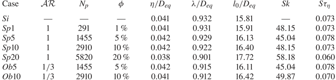
Table 1. Parameters of the main simulation cases:  $N_p$ denotes the number of particles; $l_0 \equiv \int _0^{\infty } k^{-1} E(k) \, \textrm {d} k / \int _0^{\infty } E(k) \, \textrm {d} k$ is the integral length scale, with $E(k)$ the energy spectrum at each wavenumber $k$;
$k$;  $Sk = \tau _p / \tau _{\eta }$ denotes the Stokes number, with $\tau _p = (\rho _f + 2 \rho _p) D_{eq}^{2} / (36 \rho _f \nu )$ the particle response time and $\tau _{\eta } = (\nu / \epsilon )^{1/2}$ the Kolmogorov time scale. The reported quantities are statistically averaged when the flow has reached the stationary state.
2.4. Validation and characteristics of statistically stationary state
To test the numerical code for the specific case of HST, the single-phase HST case  $Si$ is assessed against the results of Pumir (Reference Pumir1996). The initial homogeneous isotropic turbulence field, described in the previous section, is subjected to the shear rate $S$ at $St=0$ and statistics are collected afterwards. Figure 1(a) shows the time history of the box-averaged turbulent kinetic energy (black line) and enstrophy $\Omega =\langle \omega _i \omega _i \rangle$ (green line), normalised by their time-averaged values. Two distinct states are distinguishable through the time evolution of the flow. First, until $St \approx 30$, the turbulent kinetic energy grows faster than enstrophy, which indicates excess production over dissipation. After the initial transient state, the flow reaches a statistically stationary state when the production and the dissipation rates of the turbulent energy are almost in balance. This is characterised by a sequence of spikes of the turbulent energy, followed by spikes of enstrophy with a delay of approximately $5 St$, which is evident in our results and in those of Pumir (Reference Pumir1996).
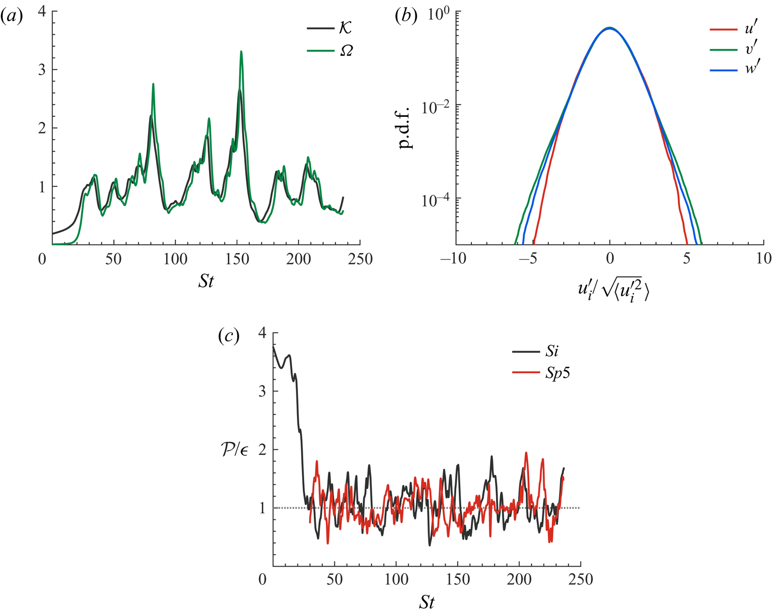
Figure 1. (a) Time history of the turbulent kinetic energy  $\mathcal {K} = \langle u_i^{\prime }u_i^{\prime }\rangle /2$ (black line) and enstrophy $\Omega$ (green line), normalised by their mean values. (b) Probability density function (p.d.f.) of the streamwise (blue), normal (red) and spanwise (green) components of the velocity, normalised by their r.m.s. values for the case $Si$. (c) Time history of the ratio between the turbulent production $\mathcal {P} = - S \langle u^{\prime } v^{\prime } \rangle$ and the turbulent dissipation rate $\epsilon = \mu \langle \partial u_i^{\prime } / \partial x_j \partial u_i^{\prime } / \partial x_j \rangle$ for the cases $Si$ (black) and $Sp5$ (red).
Figure 1(b) shows the normalised probability density function of the velocity components. The figure shows that the distributions of the normal and spanwise components have more extended tails than that of the streamwise component. This is in agreement with the results of Pumir (Reference Pumir1996), suggesting that the strong anistropy may arise from the anisotropic forcing of HST. In particular, we simulated Run No.  $2$ in Pumir (Reference Pumir1996) in a cubic box with $256$ grid points in each direction. The velocity anisotropy tensor components $b_{ij} = \langle u^{\prime }_i u^{\prime }_j / u^{\prime }_k u^{\prime }_k - \delta _{ij}/3\rangle$ in our simulation are $b_{11} = 0.231$, $b_{22} = 0.129$ and $b_{12}=0.147$, and have a maximum difference below $5\,\%$ from those reported in the cited reference.
When the single-phase case  $Si$ reaches the statistically stationary state, in which the production and the dissipation rates of the turbulent kinetic energy are statistically in balance $\mathcal {P} \approx \epsilon$ (see the black line in figure 1c), the flow field is used to initialise the multiphase cases. At this point, the turbulence flow parameters evolve from the initial values to $Re_{\lambda } = 103$ and $S^{\ast } = 2.4$. The rigid particles are introduced randomly with volume fraction ranging from $1\,\%$ to $20\,\%$. The time history of the ratio between the production and the dissipation rates of the turbulent kinetic energy for case $Sp5$ (the red line in figure 1c) confirms that the stationary state is not exclusive to the single-phase HST; after the introduction of the dispersed phase, the flow goes through a relatively short transient state and reaches a second steady state, in which the production and the dissipation rates of the turbulent energy are statistically in balance. In their recent study, Rosti etal. (Reference Rosti, Ge, Jain, Dodd and Brandt2019) documented the existence of a steady state in the presence of deformable droplets for a similar initial field and geometry.
3. Results
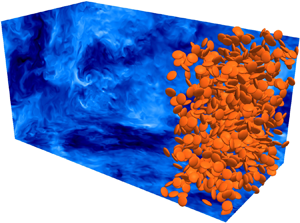
We start by showing snapshots of the flow field and particles. In figure 2 we show the two cases  $Sp10$ and $Ob10$, with the instantaneous streamwise velocity $u^{\prime }$ contours depicted on the vertical and horizontal planes. Only particles with streamwise centre coordinate larger than $0.75 L_x$ are shown in the figure for better clarity. We observe that the level of the streamwise fluctuations is higher for the case of oblates, suggesting higher turbulent activity and hence $Re_{\lambda }$. Also, more distinct patches of low-speed velocity fluctuations are present for the case $Ob10$ compared to $Sp10$.

Figure 2. Instantaneous contours of the streamwise velocity  $u^{\prime }$ on the orthogonal planes $xy$,
$xy$,  $xz$ and $yz$ for the cases $Sp10$ (a) and $Ob10$ (b); for clarity, only particles with streamwise location larger than $0.75 L_x$ are shown.
3.1. Turbulence modulation
In this first section, we quantify the turbulence modulation by the presence of the particles by discussing the statistically averaged flow parameters for all the cases. The averaged Eulerian fluid statistics reported here correspond to mean intrinsic averages. The intrinsic average of a quantity  $\xi$ is computed as
 \begin{equation} \langle \xi\rangle = \dfrac{\displaystyle\sum_{ijk,t}\xi_{ijk,t}\Psi_{ijk,t}}{\displaystyle\sum_{ijk,t}\Psi_{ijk,t}}, \end{equation}
where  $\Psi _{ijk,t}$ is the fluid volume fraction at the grid cell $ijk$ and instant $t$.
$t$.
Figure 3(a) depicts the Taylor microscale Reynolds number  $Re_{\lambda }=(2\mathcal {K}/3)^{1/2} \lambda / \nu$ as a function of the particle volume fraction $\phi$. The results show that increasing the volume fraction of spheres up to $\phi =10\,\%$ decreases $Re_{\lambda }$ with respect to the single-phase flow. However, at $\phi =20\,\%$ a considerable jump ( $\approx 17\,\%$) in $Re_{\lambda }$ is observed, indicating a non-monotonic effect of the volume fraction. The same behaviour can also be observed for the oblate particles, with the increase in $Re_{\lambda }$ happening at a lower volume fraction, i.e. $Re_{\lambda }$ is lower for $Ob5$ compared to $Sp5$, but attains a higher value than single phase ( $Si$) and $Sp10$ at a concentration of 10 % ( $Ob10$).
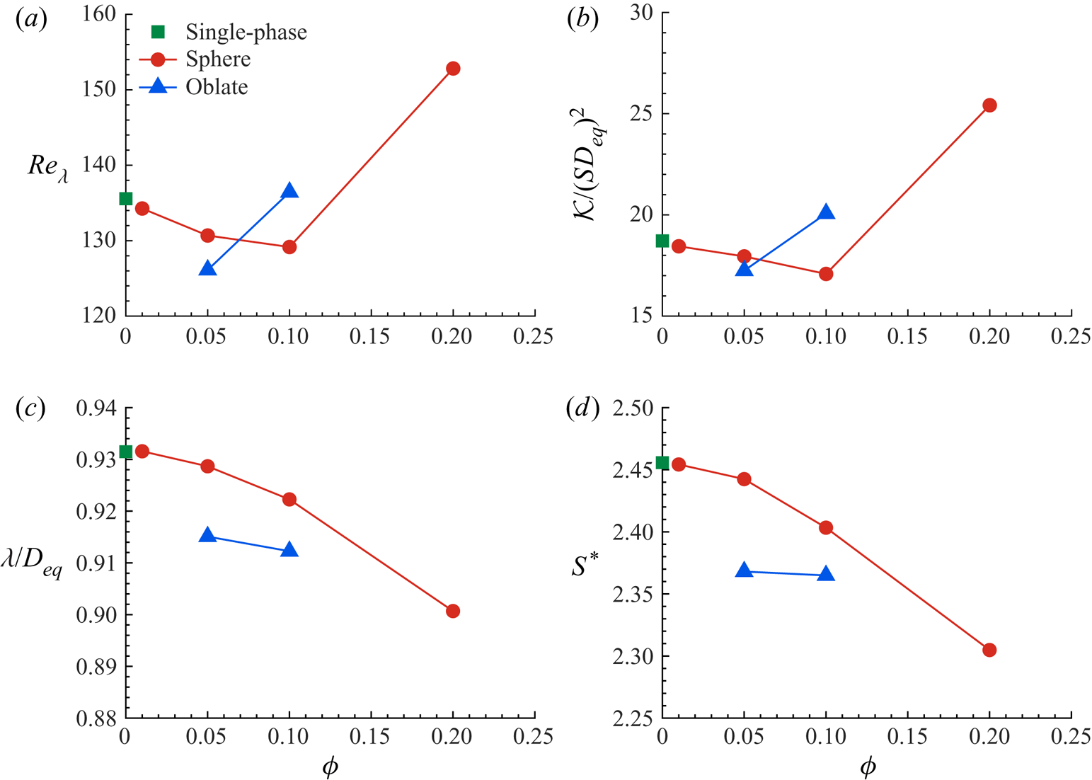
Figure 3. (a) Taylor microscale Reynolds number, (b) normalised turbulent kinetic energy  $\mathcal {K}$, (c) Taylor microscale $\lambda$ and (d) shear-rate parameter $S^{\ast }$ as a function of $\phi$.
Figure 3(b,c) displays the change of the turbulent kinetic energy  $\mathcal {K} = \langle u_i^{\prime }u_i^{\prime }\rangle /2$ and of the Taylor microscale $\lambda = \sqrt []{10 \nu \mathcal {K} / \epsilon }$, the two parameters defining $Re_{\lambda }$, as a function of the solid volume fraction. The data reveal that the variation of $Re_{\lambda }$ can be mainly attributed to the modulation of the turbulent energy by the particles, as $\mathcal {K}$ shows the same trend as $Re_{\lambda }$ (cf. figure 3a). The Taylor microscale $\lambda$, conversely, decreases monotonically with increasing volume fraction for all the cases; this variation, however, is only $\sim$3 %. Note that a reduction of the turbulent energy in a dilute suspension of rigid spheres ( $\phi = 0.5\,\%$) was also observed in the study by Tanaka & Teramoto (Reference Tanaka and Teramoto2015) in transient HST. Those authors show that the increase of the viscous dissipation is responsible for the decrease of the turbulent energy.
Finally, figure 3(d) shows the variation of the shear-rate parameter  $S^{\ast }= 2 S \mathcal {K} / 3 \epsilon$ as a function of the volume fraction for all cases under consideration. The trend is similar to that of the Taylor microscale that can be seen in figure 3(b). The shear-rate parameter is defined using the dissipation length $l_d = (2 \mathcal {K})^{3/2} / \epsilon$, the length scale associated with energy-containing eddies (Lee etal. Reference Lee, Kim and Moin1990). Therefore, we infer from figure 3(c,d) that the length and time scales of the energy-containing eddies are decreasing with increasing solid volume fraction.
The averaged spectra of the turbulent kinetic energy are reported in figure 4. As expected, we observe a range at intermediate wavenumbers where  $E \propto k^{-5/3}$, similar to that found in the logarithmic layer of wall-bounded flows (Sekimoto etal. Reference Sekimoto, Dong and Jiménez2016). Nonetheless, the presence of the solid particles has a significant effect on the energy spectrum; they increase the energy level at large wavenumbers (small scales), while they slightly reduce the energy of the low-wavenumber (large) structures. This effect is amplified by increasing the volume fraction of the solid phase, while the shape effects (spherical versus oblate particles) are observed to be rather negligible. The characteristics of the energy spectrum are similar to the observations of Lucci etal. (Reference Lucci, Ferrante and Elghobashi2010) for solid particles in decaying homogeneous isotropic turbulence and Rosti etal. (Reference Rosti, Ge, Jain, Dodd and Brandt2019) for droplets in HST; the spectrum modifications have been attributed to the breakup of the large eddies and to the increase of the frequency of the small eddies as a result of the presence of the dispersed phase.
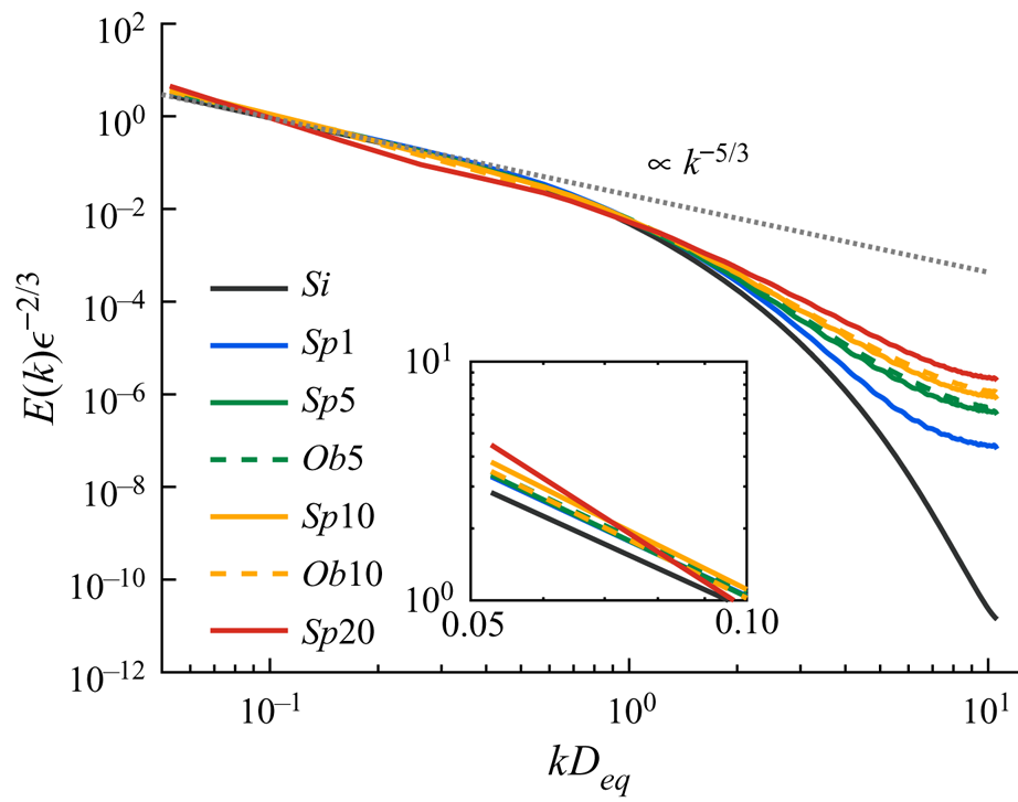
Figure 4. Spectra of the mean turbulent kinetic energy. The inset shows a magnified view of the smallest wavenumbers (largest structures).
The probability distributions of the fluctuating quantities are of obvious interest in the study of turbulent flows. Therefore, we compare the p.d.f. of the normalised velocity components for the different cases under investigation in figure 5. The values of the first four central moments of the p.d.f.s, shown in figure 5, are reported in table 2 in the appendix. First, it is worth noticing that all the multiphase cases show anisotropy in the fluid velocity fluctuations, similarly to the single-phase HST statistics reported in the literature (see e.g. Pumir Reference Pumir1996), i.e. the streamwise component has a higher root-mean-square (r.m.s.) value than the normal and spanwise ones. Interestingly, the difference between the spanwise and the normal components of the fluid velocity increases in the presence of the solid particles (cf. figure 1b).
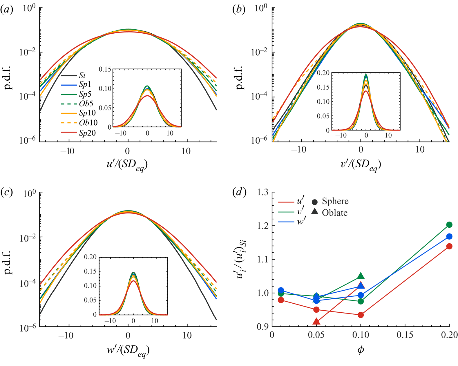
Figure 5. The p.d.f. of the normalised velocity components: (a) streamwise, (b) normal and (c) spanwise; the insets show the p.d.f.s in linear scale. (d) The averaged velocity components normalised by the single-phase value  $(u^{\prime }_i)_{Si}$.
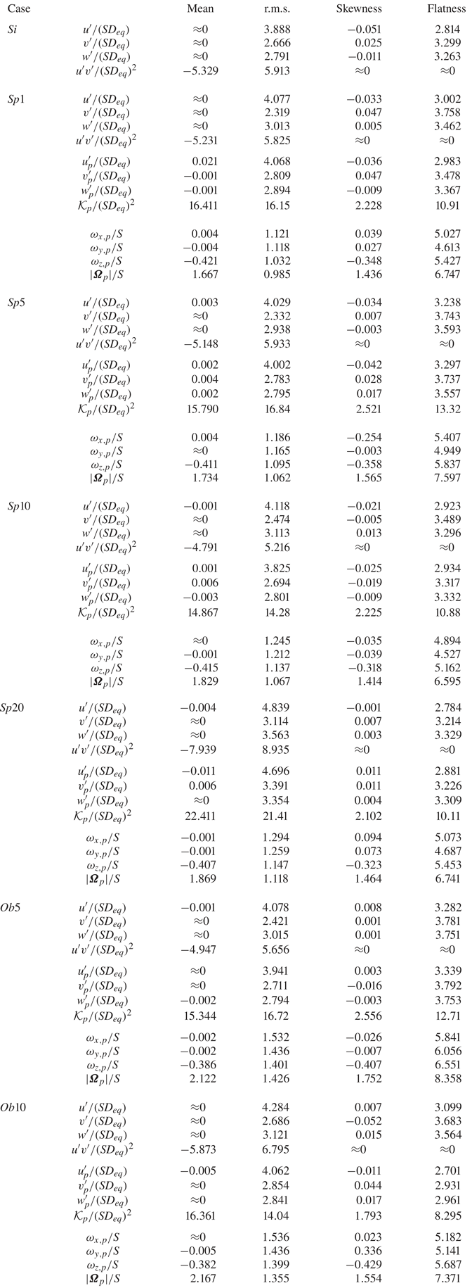
Table 2. First four central moments of the density probability functions of the fluid and particle velocity components, together with the Reynolds shear stress  $u^{\prime }v^{\prime }$, the particle kinetic energy and magnitude of the angular velocity vector for different cases. Values smaller than $10^{-3}$ in magnitude are set to zero.
To understand the role of particle volume fraction, we first compare the cases laden with spherical particles. Up to  $\phi =10\,\%$, the normal velocity has a similar distribution to the single-phase HST, whereas the streamwise and spanwise components have stronger tails. Increasing the volume fraction to $20\,\%$ leads to an increase in the probability of strong fluctuations in all velocity components, which consequently results in a higher magnitude of the turbulent kinetic energy and $Re_{\lambda }$. On the other hand, the main difference for oblate particles is in the distribution of the normal velocity for $\phi =10\,\%$, where the probability of extreme fluctuations has increased significantly. The higher value of the p.d.f. in the range $|v^{\prime }| / (SD_{eq}) > 5$ again results in the higher values of the turbulent energy and $Re_{\lambda }$ documented above for oblates when increasing the particle volume fraction.
This can also be observed in figure 5(d), where the r.m.s. velocity fluctuations are averaged and depicted for all the cases under investigation. Interestingly, the effect of the volume fraction is more pronounced on  $u^{\prime }$ than on the normal and spanwise components of the velocity fluctuations for spheres up to $\phi =10\,\%$ and for oblates at $\phi =5\,\%$, i.e. the reduction of the turbulent energy for these cases is associated with the reduction of $u^{\prime }$ rather than of the two cross-stream components. However, for cases $Sp20$ and $Ob10$ all the components experience a significant increase with respect to the single-phase case, owing to the long tails of the p.d.f.s. The relation between these results and the particle dynamics will be explained in § 3.2.
Thus far, we have discussed the modification of the fluctuating velocities and related parameters to quantify the turbulence modulation by the presence of the particles. To have a better picture of the events responsible for the modification of the turbulence, we present the weighted Reynolds shear stress contours, computed by multiplying the absolute value of the Reynolds shear stress by the joint probability density of its occurrence in the  $u^{\prime }\text {--}v^{\prime }$ plane (Zhou etal. Reference Zhou, Adrian, Balachandar and Kendall1999). This method considers the contribution of the different events to the total stress by locating them on the four quadrants of the $u^{\prime }\text {--}v^{\prime }$ plane, denoted $Q_{1\text {--}4}$. The events on the $Q_2$ ( $u^{\prime } < 0$, $v^{\prime } > 0$) and $Q_4$ ( $u^{\prime } > 0$, $v^{\prime } < 0$) quadrants result in production of turbulence, whereas $Q_1$ ( $u^{\prime } > 0$, $v^{\prime } > 0$) and $Q_3$ ( $u^{\prime } < 0$, $v^{\prime } < 0$) are responsible for attenuation.
The contours of the weighted Reynolds shear stress, statistically averaged in the fluid phase for all the cases, are displayed in figure 6. For all cases, the diagrams are symmetric with respect to the origin, which fulfils the symmetry of the HST under the transformation  $(x,y,z) \to (-x,-y,z)$, and, expectedly, confirms that the inhomogeneity observed in the quadrant analysis of the wall-bounded flows (see e.g. Wallace Reference Wallace2016) vanishes in unbounded ones. Figure 6(a–d) shows the results for the cases laden with spheres. For cases $Sp1$ (figure 6a), $Sp5$ (figure 6b) and $Sp10$ (figure 6c), the contribution of events $Q_2$ and $Q_4$ to the production and the quenching events $Q_1$ and $Q_3$ have not changed considerably (see iso-line of $0.6$ in figure 6a–c). The top contributor events of the $Q_2$ and $Q_4$ quadrants have higher magnitude of the streamwise component $u^{\prime }$ compared to the normal one $v^{\prime }$. Conversely, in case $Sp20$ (see figure 6d), the production associated with $Q_2$ and $Q_4$ events becomes more predominant as the magnitude of the velocity fluctuations for the top contributor events increases for both the streamwise and the normal components; at the same time, the attenuation induced by $Q_1$ and $Q_3$ events is much weaker than for the cases with lower volume fraction of spherical particles. Note also that the importance of the streamwise and normal components of the velocity vector in the production and damping mechanisms is more balanced in case $Sp20$.
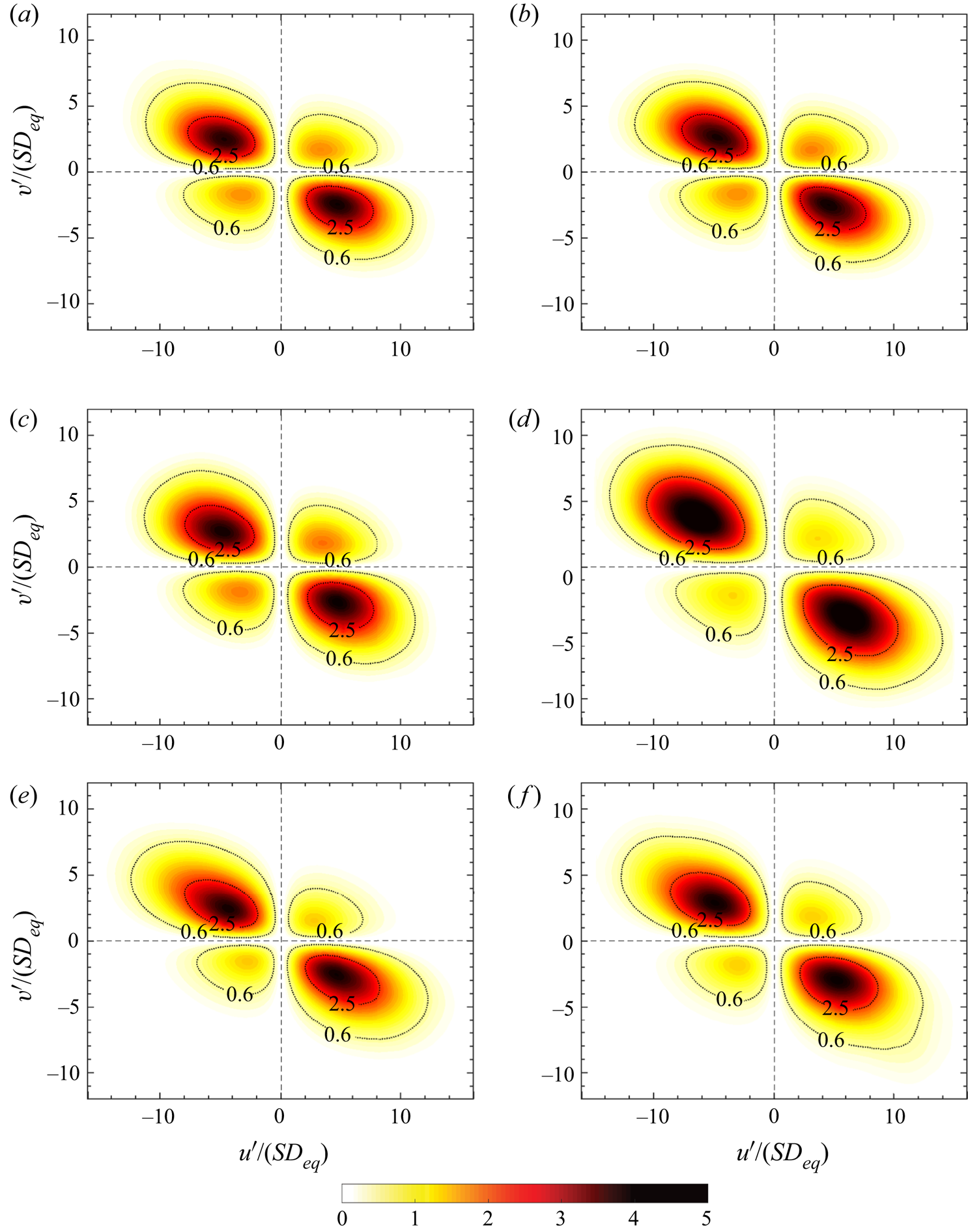
Figure 6. Contours of the weighted Reynolds shear stress, given by multiplying the absolute value of the Reynolds shear stress by the joint probability density of its occurrence in the  $u^{\prime }\text {--}v^{\prime }$ plane: (a) $Sp1$, (b) $Sp5$, (c) $Sp10$, (d) $Sp20$, (e) $Ob5$ and (f) $Ob10$.
To conclude this analysis, figure 6(e,f) displays the contours of the weighted Reynolds shear stress for cases  $Ob5$ and $Ob10$. Here, we see that the area of the contours contributing to both production and attenuation increases slightly when increasing the volume fraction, indicating the importance of the contribution from rare but highly energetic events. When comparing the flow laden with oblate particles with the case of spheres at the same volume fraction, we note that the contours are more skewed towards higher values of the velocity, which confirms the increased role of the higher-intensity events in the case of oblate particles.
3.1.1. Turbulent kinetic energy budget
To quantify the effect of the dispersed phase on the modulation of the turbulence, we look at the turbulent kinetic energy budget for the fluid phase. The governing equation for the evolution of the turbulent kinetic energy  $\mathcal {K}$ reads
 \begin{gather} \frac{ \textrm{d} \mathcal{K}}{ \textrm{d} t} = \mathcal{P} - \epsilon + \mathcal{I}, \end{gather}
 \begin{gather}\mathcal{P} = -S \langle u^{\prime} v^{\prime} \rangle, \end{gather}
 \begin{gather}\epsilon = \mu \left\langle \frac{\partial u_i^{\prime}}{\partial x_j} \frac{\partial u_i^{\prime}}{\partial x_j} \right\rangle, \end{gather}
 \begin{gather}\mathcal{I} = \langle u_i^{\prime}\, f_i \rangle, \end{gather}
where  $\mathcal {I}$ denotes the energy transfer through the interphase interaction (Tanaka & Teramoto Reference Tanaka and Teramoto2015), which can act as a source or a sink of turbulent energy (Ferrante & Elghobashi Reference Ferrante and Elghobashi2003). At the steady state, the rate of change of $\mathcal {K}$ is obviously zero and the remaining terms are in balance. For a more clear comparison, we normalise each term on the right-hand side of (3.2) by the product of the shear rate $S$ and the averaged turbulent kinetic energy of the singe-phase case $Si$:
$Si$:
 \begin{gather} \sigma_1 = \frac{\mathcal{P}}{S \mathcal{K}_{Si}} = -\frac{2 \langle u^{\prime} v^{\prime} \rangle}{\langle u_k^{\prime}u_k^{\prime}\rangle_{Si}}, \end{gather}
 \begin{gather}\sigma_2 = -\frac{\epsilon}{S \mathcal{K}_{Si}} =-\frac{2 \epsilon}{S \langle u_k^{\prime}u_k^{\prime} \rangle_{Si}}, \end{gather}
 \begin{gather}\sigma_3 = \frac{\mathcal{I}}{S \mathcal{K}_{Si}} =\frac{2 \langle u_k^{\prime} f_k \rangle}{S \langle u_k^{\prime}u_k^{\prime} \rangle_{Si}}. \end{gather}
The relative contribution of each term  $\sigma _{1\text {--}3}$ to the turbulent kinetic energy budget for all the cases under consideration is displayed in figure 7. The data reveal that the production and the dissipation rates are almost in perfect balance for all cases, and that the contribution of the interphase interaction term is less than $3.5\,\%$ of the total. Note that despite the very small contribution of $\sigma _3$, its presence is necessary to have a correct energy balance. Also, the presence of the solid phase affects the production and dissipation rates of the turbulent kinetic energy, i.e. the variations of $\sigma _1$ and $\sigma _2$ due to the presence of particles. Comparing to the single-phase case $Si$, the production and the dissipation rates decrease and the interphase interaction increases monotonically with the sphere volume fraction for $\phi \le 10\,\%$, whereas at $\phi \le 20\,\%$ the production and the dissipation rates are greater than in the single-phase flow and the interphase interaction contributes to the production of the kinetic energy, instead of being a sink of energy as at lower volume fractions.
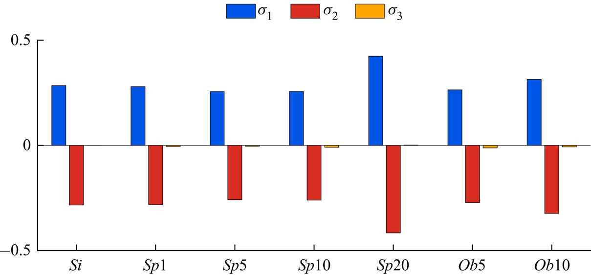
Figure 7. Contribution of turbulent production  $\mathcal {P}$, dissipation rate $\epsilon$ and the interphase interaction term $\mathcal {I}$ to the turbulent kinetic energy budget for the different cases under consideration. Each term is normalised by the product of the shear rate $S$ and the averaged turbulent kinetic energy of the single-phase case $Si$.
$Si$.
In the case of the oblate particles, the same trend is observed at lower volume fractions, i.e. case  $Ob10$ has greater production and dissipation rates than cases $Ob5$ and $Si$, and the contribution of the interphase interaction to the dissipation of the kinetic energy is lower.
3.2. Particle dynamics
In this section, we investigate the link between the dynamics of the particles and the modulation of the turbulence by examining the Lagrangian statistics of the solid particles. Figure 8(a) displays the normalised translational kinetic energy of the solid particles, defined as  $\mathcal {K}_p \equiv 0.5 (u_p^{\prime 2} + v_p^{\prime 2} + w_p^{\prime 2})$, as a function of the volume fraction $\phi$, whereas figure 8(b) depicts $\mathcal {K}_p$ normalised by the turbulent kinetic energy of the carrier fluid. The amplitude of the particle velocity fluctuations follows the same trend as that of the carrier fluid, displayed in figure 3(b). The kinetic energy of the spherical particles first decreases when increasing the solid volume fraction until $\phi =10\,\%$, and then increases significantly when the volume fraction is increased to $\phi =20\,\%$. In the case of oblate particles, the increase of the particle kinetic energy occurs at a lower volume fraction, and in fact we only observe an increase of $\mathcal {K}_p$ for the two volume fractions considered here, $\phi =5\,\%$ and $10\,\%$. Scaling the particle kinetic energy by the turbulent kinetic energy of the carrier fluid (cf. figure 8b), we see that rigid particles tend to fluctuate less than the fluid. This is similar to the results of Tanaka & Teramoto (Reference Tanaka and Teramoto2015), who show that the ratio between the magnitude of the fluctuating particle velocity and that of the fluid for dilute suspensions of spherical particles in transient HST is around $0.85$, and to the observations of Picano etal. (Reference Picano, Breugem and Brandt2015) for a channel flow laden with neutrally buoyant spherical particles for the region which lies in the near-wall range $30 < y^{+} < 70$ in inner units. By comparing figures 8(a) and 8(b), we infer that increasing the volume fraction of the solid particles, for spheres from $10\,\%$ to $20\,\%$ and for oblates from $5\,\%$ to $10\,\%$, has a larger impact on the increase of the fluid velocity fluctuations than on that of the particle velocity fluctuations.
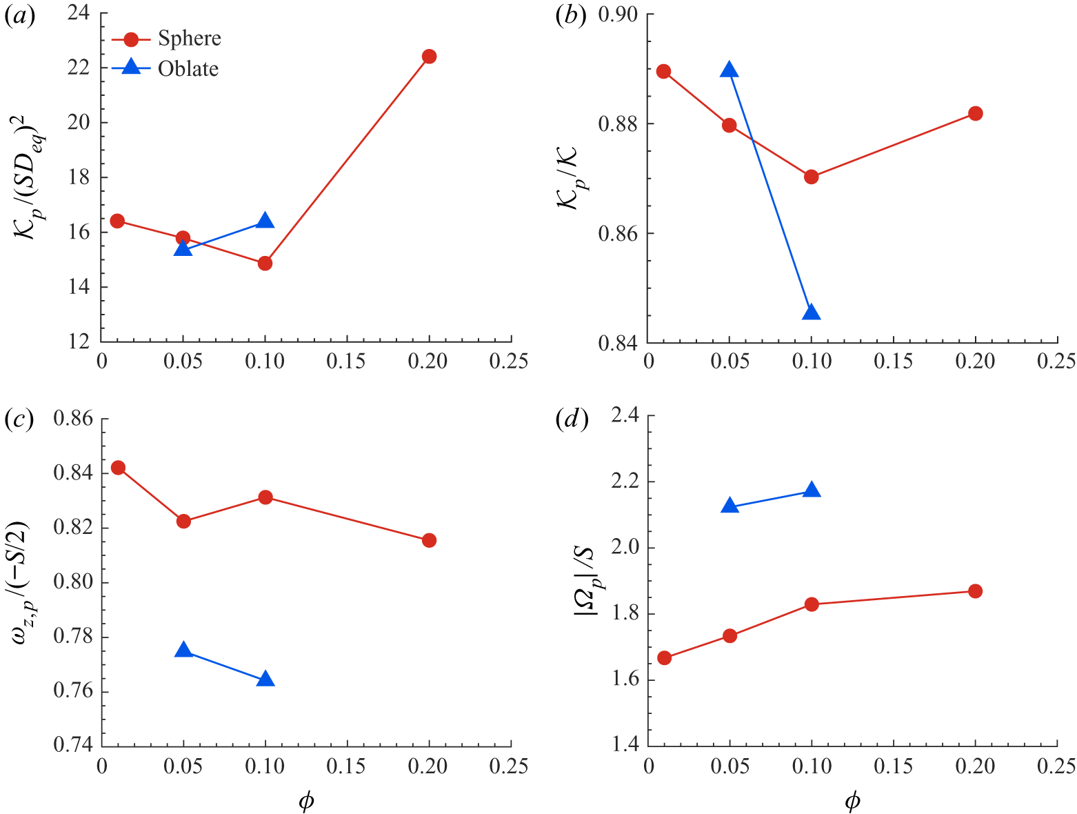
Figure 8. (a) Normalised translational kinetic energy of the particles  $\mathcal {K}_p = 0.5 (u_p^{\prime 2} + v_p^{\prime 2} + w_p^{\prime 2})$, (b) $\mathcal {K}_p$ normalised by the turbulent kinetic energy of the carrier fluid, (c) the spanwise angular velocity of the particles normalised by the angular velocity of the mean shear flow and (d) the magnitude of the average particle angular velocity vector $|\boldsymbol {\Omega }_p| = \sqrt {\omega _{x,p}^{2} + \omega _{y,p}^{2} + \omega _{z,p}^{2}}$ as a function of the volume fraction. Symbols and colour scheme as in figure 3.
The spanwise component of the particle mean angular velocity, normalised by the rotation associated with the mean shear flow  $-S/2$, is displayed in figure 8(c). First, note that the average spanwise rotation rates are around $8\,\%$ more for the spheres than for the oblates. Moreover, for both spheres and oblates, the changes of the averaged spanwise angular velocity by the increase of the volume fraction $\phi$ do not show a clear trend. The value obtained by Tanaka & Teramoto (Reference Tanaka and Teramoto2015) for spherical particles in the dilute regime in transient HST is around $0.9$, larger than those obtained here at higher $\phi$. Finally, the magnitude of the particle angular velocity vector $|\boldsymbol {\Omega }_p| = \sqrt {\omega _{x,p}^{2} + \omega _{y,p}^{2} + \omega _{z,p}^{2}}$ is shown in figure 8(d). The rotation rate $|\boldsymbol {\Omega }_p|$ is around $20\,\%$ larger for the oblates than for the spheres and an increase of the volume fraction of the solid particles only slightly increases its value. A comparison between figures 8(c) and 8(d) reveals that the oblate particles have larger angular momentum in the shear-plane directions than spherical particles and also have a clearer tendency to rotate opposite to the mean shear flow vorticity vector (see figure 10c).
Next, we wish to give further insight into the behaviour of the solid phase by examining the velocity probability functions. To this end, we display in figure 9 the p.d.f.s of the three particle velocities (figure 9a–c) together with that of the particle translational kinetic energy  $\mathcal {K}_p$ (figure 9d); see table 2 in the appendix for the values of the different statistical moments. Note that since particles have a considerable size with respect to the flow structures ( $D_{eq} \approx 25 \eta$) and follow a rigid-body motion, they are able to couple the fluctuations of the fluid velocity in the cross-flow directions, which therefore exhibit a more isotropic behaviour. This is evident in table 2 in the appendix, where the r.m.s. of the particle velocity fluctuations in the cross-flow directions are shown to assume values approximately equal to the average of the r.m.s. of the normal and spanwise fluid velocity fluctuations. Moreover, we observe no significant change in the distributions of the normal and spanwise components of the particle velocity when increasing the volume fraction of the spherical particles up to $\phi =10\,\%$, so that the decrease of the translational kinetic energy of the particles $\mathcal {K}_p$ (figure 9d) can be associated with the decrease of the streamwise component (figure 9a). At the highest volume fraction considered, $\phi =20\,\%$ (case $Sp20$), however, we observe an increase in all the p.d.f.s of the velocity components in the range $5 < |u_{p,i} / (SD_{eq})| < 10$. This isotropic increase in all components can be an indication that at this solid-phase concentration, particle–particle interactions become relevant. The effect of the shape of the particles is evident comparing the distributions for the cases $Sp10$ and $Ob10$. The data indicate a higher probability of larger values of the particle translational kinetic energy in the range $100 < \mathcal {K}_p / (SD_{eq})^{2} < 200$ in the flow laden with oblate particles, which relates to the higher probability of extreme fluctuations of the streamwise velocity component $u^{\prime }_p$.
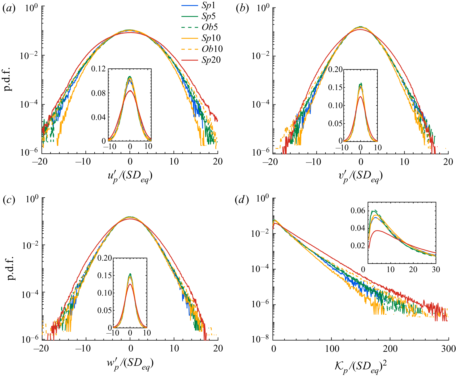
Figure 9. The p.d.f.s of the particle velocity: (a) streamwise, (b) normal and (c) spanwise components. (d) The p.d.f. of the particle translational kinetic energy  $\mathcal {K}_p$. The insets show the p.d.f.s in linear scale.
The p.d.f.s of the components of the particle angular velocity are displayed in figure 10(a–c), whereas that of the magnitude of the angular velocity vector  $|\boldsymbol {\Omega }_p|$ is shown in figure 10(d); the values of the statistical moments can be found in table 2 in the appendix. The data in the figure reveal that an increase of the volume fraction alone only extends the tails of the p.d.f.s slightly, while the shape of the particles has a more noticeable effect, i.e. the cases laden with oblate particles have significantly longer tails compared to the cases with spheres. The spanwise angular velocity of the particles is of particular interest, as this is driven by the imposed shear. The p.d.f.s are clearly skewed towards negative values, which indicates that particles, expectedly, rotate in the direction imposed by the mean shear for most of the instances; the mean values are reported in table2 in the appendix. One can also note that oblates happen to rotate opposite to the direction of the angular velocity of the mean shear more frequently and at higher rates; this explains why they have lower averaged values of $\omega _{z,p}$ than spheres, as shown in figure 8(c).

Figure 10. The p.d.f.s of the particle angular velocity: (a) streamwise, (b) normal and (c) spanwise components. (d) The p.d.f. of the magnitude of the particle angular velocity vector  $|\boldsymbol {\Omega }_p|$. The insets show the p.d.f.s in linear scale.
Next, we investigate possible particle clustering by computing the pair distribution function  $P(\boldsymbol {r})$, which denotes the conditional probability of finding a particle at distance $\boldsymbol {r}$ given one at the origin (see e.g. Kulkarni & Morris Reference Kulkarni and Morris2008):
 \begin{equation} P(\boldsymbol{r}) = P(r, \theta, \psi) = \frac{H(r, \theta, \psi)}{n t_s {\rm \Delta} V}, \end{equation}
where  $\theta$ is the polar angle measured from the positive $z$ axis, $\psi$ is the azimuthal angle measured counterclockwise from the positive $x$ axis, $n$ is the average particle number density, $t_s$ is the total number of sampling points, ${\rm \Delta} V = r^{2} \sin (\theta ) {\rm \Delta} \theta {\rm \Delta} \psi {\rm \Delta} r$ is the volume of the sampling bin and $H(r, \theta , \psi )$ is the histogram of particle pairs. More specifically, the particle-pair histogram $H(r, \theta , \psi )$ is progressively built by discretising the pair space in $r$,
$r$,  $\theta$ and $\psi$ and putting each separation vector $\boldsymbol {r}$ into the corresponding bin of size ${\rm \Delta} V$ at each sampling time.
The pair distribution function has been calculated in a spherical shell with diameter of  $5D_{eq}$ around the mass centre of the particles and displayed in figure 11, where the data are shown in the $x$–
$x$– $y$ plane ( $\theta ={\rm \pi} /2$) for the cases $Sp10$, $Sp20$ and $Ob10$. Note that in this figure and subsequent sections, the oblate particles are visualised by a sphere with a diameter equal to their minor axis. All panels show a relative accumulation of particles in the compressional quadrants and a depletion in the extensional quadrants, similar to results from previous experiments and simulations of suspensions in simple shear flow at low Reynolds number (Morris Reference Morris2009). On increasing the volume fraction, the narrow strips with high values of $P$ become more uniform around the surface of the particle (see figure 11b). This can be another indication that at $\phi =20\,\%$, particle–particle interactions significantly affect the particle dynamics. In the case of oblates, the contour levels are below unity around the reference particle and no clustering is observed (see figure 11c). Still, the contours of $P$ have lower values in the extensional quadrants compared to compressional ones. The absence of clustering together with the higher probability of extreme events observed in the p.d.f.s of the linear and angular velocities of the oblates can be indicative of strong collisions between them, as they depart rapidly after contact.

Figure 11. Pair distribution function  $P(r, \psi )$ in the plane normal to the spanwise direction $(\theta ={\rm \pi} /2)$ for the cases (a) $Sp10$, (b) $Sp20$ and (c) $Ob10$.
The dynamics of the particle pairs is not only determined by their relative position, i.e. by the pair distribution function, but also by their relative velocity (Lashgari etal. Reference Lashgari, Picano, Breugem and Brandt2016). Following the study by Sundaram & Collins (Reference Sundaram and Collins1997), we therefore compute the normal relative velocity of the particle pairs as a function of the separation distance  $r$ (the distance between the centres). Considering particles $p$ and $q$, the normal relative velocity of the particle pair is obtained as the inner product of their relative velocity and relative distance:
 \begin{equation} {\rm \Delta} v_n(r_{p,q}) = (\boldsymbol{u}_p - \boldsymbol{u}_q) \boldsymbol{\cdot} \frac{(\boldsymbol{r}_p - \boldsymbol{r}_q)}{|(\boldsymbol{r}_p - \boldsymbol{r}_q)|}. \end{equation}
 The normal relative velocity can be either negative,  ${\rm \Delta} v_n^{-}$, for approaching particles or positive, ${\rm \Delta} v_n^{+}$, when the two particles depart from each other. Figure 12 shows the magnitude of the negative relative velocity $| {\rm \Delta} v_n^{-} |$ as a function of the separation distance $r$ for some different cases. The relative velocity increases almost monotonically with $r$ as the pairs are more likely to approach with higher velocity when farther away. The approaching velocities are observed to increase slightly with increasing volume fraction, meaning that particles experience stronger pair interactions at higher volume fractions. Note that the abrupt decrease of the approaching velocity for separation distances close to $r/D_{eq} = 1$ shows the effect of the lubrication force on the dynamics of the spherical particles. In addition, oblate particles can get closer to each other ( $r/D_{eq} < 1$) due to their shape, while maintaining high relative velocities. This creates stronger pair interactions for oblate particles, resulting in higher turbulent kinetic energy when the number of pair interactions increases (high volume fractions).

Figure 12. Magnitude of relative (approaching) normal velocity  $| {\rm \Delta} v_n^{-} |$ as a function of the separation distance between particle pairs.
To better characterise the effect of the shape of the particles, we examine the orientation with respect to the underlying flow of the oblate particles. Figure 13(a) shows the p.d.f.s of the magnitude of the components of the unit vector associated with the particle symmetry axis  $\boldsymbol {\hat {o}} = (\hat {o}_x, \hat {o}_y, \hat {o}_z)$ for the cases $Ob5$ and $Ob10$. The data reveal that oblate particles have an almost random distribution of orientations, with a weak tendency to be aligned with the normal and the spanwise directions. Figure 13(b) shows the orientation correlation function $OCF(r)$, which quantifies the relative orientation of close particles:
 \begin{equation} OCF(r) = \langle 2 | \boldsymbol{\hat{O}}_p \boldsymbol{\cdot} \boldsymbol{\hat{O}}_q | - 1 \rangle, \end{equation}
where  $\boldsymbol {\hat {O}}_p$ and $\boldsymbol {\hat {O}}_q$ denote the orientation of particles $p$ and $q$ at distance $r$ between their centres. The value $OCF(r)=0$ indicates a suspension with random particle orientation, while $OCF(r) = 1$ means particle pairs at distance $r$ perfectly aligned. The results show that oblate particles tend to be more aligned with each other for separation distances in the range $0.5 < r/D_{eq} < 1.5$, i.e. as long as they are in contact with each other they move as a small cluster with similar alignment – something that, however, the data in figure 11(c) show to happen rarely. The correlation function vanishes very quickly when increasing the separation distance, showing decorrelation in the alignment of the particles for distances above $1.5D_{eq}$. Ardekani etal. (Reference Ardekani, Costa, Breugem, Picano and Brandt2017) performed the same analysis for oblate particles in a turbulent channel flow. Those authors showed that the correlation distance is significantly smaller in the core of the channel, compared to the near-wall particles experiencing strong shear. The data in figure 13(b) are comparable to the results of the wall-bounded flow for particles in the core region, indicating the negligible effect of the mean shear on the particle orientation.

Figure 13. (a) The p.d.f. of the magnitude of the components of the unit vector associated with the particle symmetry axis  $\boldsymbol {\hat {o}} = (\hat {o}_x, \hat {o}_y, \hat {o}_z)$. (b) Orientation correlation function $OCF(r)$ versus centre separation $r/D_{eq}$.
3.3. Flow statistics around particles
In this section, we focus on the conditionally averaged flow statistics around the surface of the particles. The ensemble averaging is carried out in a cubic box of side  $3D_{eq}$ around the mass centre of the particles with a frequency of $0.5 St$ (one sample every $0.5 St$) and a total duration of $\sim 150St$, after the statistically steady state has been reached. For normalisation, a space averaging has also been carried out in the cubic box of side $3D_{eq}$ around the particles in addition to the ensemble averaging, and the averaged quantities are denoted by $\langle \boldsymbol {\cdot } \rangle _{sur}$.
Figure 14 shows contours of the turbulent kinetic energy  $\mathcal {K}$ (figure 14a–c), the turbulent production $\mathcal {P}$ (figure 14d–f) and the dissipation rate $\epsilon$ (figure 14g–i) normalised by their conditional averaged values $\langle \mathcal {K} \rangle _{sur}$, $\langle \mathcal {P} \rangle _{sur}$ and $\langle \epsilon \rangle _{sur}$, for the cases $Sp5$, $Sp20$ and $Ob5$. Contours are plotted in the $x$–
$x$– $y$ plane passing through the centre of the reference particle. Figure 14(a–c) shows therefore the modulation of the turbulent kinetic energy around the surface of the particles. The iso-contours of $\mathcal {K} / \langle \mathcal {K} \rangle _{sur}$ form almost spherical shells around the surface of the particles and are slightly elongated towards the compressional quadrants. The value of $\mathcal {K} / \langle \mathcal {K} \rangle _{sur}$ is around $0.88$ close to the surface of the particles and goes asymptotically to $1$ over a distance of $\approx 0.45D_{eq}$.

Figure 14. Contours of the conditionally averaged statistics around the particles in the  $x$–
$x$– $y$ plane. (a–c) The turbulent kinetic energy $\mathcal {K}$, (d–f) the production $\mathcal {P}$ and (g–i) the dissipation rate $\epsilon$ for cases (a,d,g) $Sp5$, (b,e,h) $Sp20$ and (c,f,i) $Ob5$. The results are normalised by their conditionally averaged values for each case, denoted by $\langle \boldsymbol {\cdot } \rangle _{sur}$.
Figure 14(d–f) shows the contours of the production  $\mathcal {P}$ and figure 14(g–i) those of the dissipation rate $\epsilon$. The production is stronger in the extensional quadrants with a value of $\mathcal {P} / \langle \mathcal {P} \rangle _{sur} = 1.1$ for the spheres and $1.3$ for the oblates close to the surface of the particles. On the other hand, in the compressional quadrants the production is lower than the mean value and is reduced to $\mathcal {P} / \langle \mathcal {P} \rangle _{sur} = 0.85$ for the spheres and $0.7$ for the oblates.
As regards the dissipation, previous experimental and numerical studies have shown that the energy dissipation is locally enhanced near the surface of the particles (see e.g. Lucci etal. Reference Lucci, Ferrante and Elghobashi2010; Tanaka & Eaton Reference Tanaka and Eaton2010). Our results (see figure 14g–i) show the same trend. The dissipation rate  $\epsilon$ is enhanced near the surface of the particles and reaches values five times larger than the mean value in the compressional quadrants in the case of spherical particles. The enhancement of the dissipation rate is more uniform around the surface of the oblates with a value of $\epsilon / \langle \epsilon \rangle _{sur} \approx 2.3$ uniformly in all directions. Tanaka (Reference Tanaka2017) reported similar behaviour for the modulation of the production $\mathcal {P}$ and the dissipation rate $\epsilon$ in transient HST and dilute suspensions of spherical particles.
More details of the origins of flow modulation by the solid phase can be obtained by the flow structures conditionally averaged around the surface of the particles. Figure 15 shows the fluctuating velocity vectors in the  $x$–
$x$– $y$ plane, passing through the centre of the reference particle. In the plot, the velocity vectors are superposed onto the contours of the magnitude of the fluctuating velocity vector $|\boldsymbol {u}^{\prime }| = \sqrt {u^{\prime 2} + v^{\prime 2} + w^{\prime 2}}$; contours are normalised by the velocity vector magnitude, conditionally averaged in the cubic box of side $3D_{eq}$ around the particles, $\langle | \boldsymbol {u}^{\prime } | \rangle _{sur}$. Figure 15(a,b) reports the results for cases $Sp5$ and $Ob5$. For both particle shapes, four vortical structures are visible around the reference particle. To discuss these flow structures in relation to the compressional/extensional quadrants around the surface of the particle more easily, a schematic is presented in figure 15(c), where the compressional/extensional quadrants are denoted by $\chi _{1\text {--}4}$, while $\Gamma _{1\text {--}4}$ indicate the vortical structures.

Figure 15. Conditionally averaged velocity vectors in the  $x$–
$x$– $y$ plane, passing through the mass centre of the reference particles. The contours are the magnitude of the fluctuating velocity vector $|\boldsymbol {u}^{\prime }| = \sqrt {u^{\prime 2} + v^{\prime 2} + w^{\prime 2}}$, normalised by the mean value averaged in the cubic box used for the conditional averaging, showing the results for cases (a) $Sp5$ and (b) $Ob5$. (c) Schematic showing the resulting vortical structures formed from the interaction between a rotating particle and a linear shear flow; the compressional and extensional quadrants around the particle are marked by $\chi _{1\text {--}4}$ and the vortical structures by $\Gamma _{1\text {--}4}$.
Figure 15 reveals that the averaged flow field around the particle surface consists of two pairs of counter-rotating vortices, with the induced velocity field reminiscent of the one induced by the force dipole (stresslet) in the vanishing inertia regime (see e.g. Graham Reference Graham2018). As shown previously in figure 14(d–f), the production is highly modulated in all quadrants  $\chi _{1\text {--}4}$. Hence, any pair of adjacent counter-rotating spanwise vortices formed around the particle surface modulate the tangential Reynolds shear stress and the turbulence production in the area between them in all quadrants. In previous studies, Kida & Tanaka (Reference Kida and Tanaka1994) and Ahmed & Elghobashi (Reference Ahmed and Elghobashi2000) showed that in HST the regions of high energy production are mainly enclosed by quasi-streamwise counter-rotating vortices, whereas here the vortices are mainly parallel to the spanwise direction.
Further, Ahmed & Elghobashi (Reference Ahmed and Elghobashi2000) showed that particles increase the dissipation rate  $\epsilon$ by creating local velocity gradients which leads to an increase of the local strain and dissipation rates. In particular, the increase of the extensional strain has a prominent effect on the enhancement of the dissipation rate $\epsilon$, although compressive strain is also increased by the presence of the solid particles. Our results show an increase of the dissipation rate in all quadrants (see figure 14g–i), but mainly in $\chi _2$ and $\chi _4$ where the vortex pairs $\Gamma _{1\text {--}2}$ and $\Gamma _{3\text {--}4}$ are inducing extensional strain rate.
Note that for the oblate particles (figure 15b), the velocity magnitude in quadrants  $\chi _1$ and $\chi _3$ is slightly larger than that in the other quadrants. This difference appears because the dynamics of the oblate particles and the flow field around them reflect their anistropic shape; i.e. the particles sample different flow patterns based on their orientation. To demonstrate this, we display in figure 16 the joint probability density of the particle orientation and the spanwise angular velocity. Here, the horizontal axis indicates the streamwise component of the particle orientation vector multiplied by the sign function of the normal component, so that positive values correspond to instances when the oblate particles are perpendicular to the mean shear direction and negative values to instances when they are aligned with mean shear. The data in the figure reveal the higher probability of sampling particles that are inclined with the shear direction when they experience larger angular velocities. This creates a small asymmetry in the flow pattern that is superposed on top of the symmetric flow pattern that appears around the spherical particles (see figure 15a). This is consistent with the findings of Ardekani etal. (Reference Ardekani, Costa, Breugem, Picano and Brandt2017) for the force and torque experienced by oblate particles in the vicinity of a wall where the shear rate is strong.

Figure 16. Joint p.d.f. of the particle orientation (streamwise component of the particle orientation vector times the sign function of the normal one) and the particle spanwise angular velocity for the case  $Ob5$.
4. Final remarks
We have used interface-resolved simulations to study the turbulence modulation of particle-laden HST at statistically steady state. Neutrally buoyant spherical and oblate particles ( $\mathcal {AR}=1/3$) are investigated up to volume fractions of $20\,\%$ and $10\,\%$, respectively. A particle size of $\approx 20$ Kolmogorov length scales in the single-phase flow is considered, which is equal to $\lambda /D_{eq} \approx 0.9$ in terms of the Taylor microscale.
We show that a statistically steady state is not exclusive to single-phase HST as the production and dissipation rates of the turbulent kinetic energy are observed to be statistically in balance in the studied particle-laden cases. The simulations show a non-monotonic trend of the turbulent kinetic energy with increasing volume fraction. Both particle shapes decrease the turbulent kinetic energy with respect to the single phase up to a certain volume fraction before the turbulence activity enhances at higher volume fractions. This increase of the turbulent kinetic energy is observed for both spherical and oblate particles, starting, however, at a lower volume fraction for the latter ( $20\,\%$ for spheres and $10\,\%$ for oblate particles). Analysis of the turbulent kinetic energy budget shows a very similar attenuation and then an increase of the production and dissipation rates of the turbulent energy, while the contribution from the interphase interaction remains below $3\,\%$.
We have documented two main mechanisms for turbulence modulation in the presence of particles. First we show that the dissipation rate is significantly larger in the vicinity of solid particles (see figure 14) due to the enlargement of extensional strain rate in these regions (see also Ahmed & Elghobashi Reference Ahmed and Elghobashi2000). This leads to turbulence attenuation as observed in the results of this study for lower volume fractions. This is in line with the numerical study of Tanaka & Teramoto (Reference Tanaka and Teramoto2015) of transient HST, where the turbulence kinetic energy is attenuated in the dilute regime. In agreement, the additional reduction of the turbulence activity for oblate particles at lower volume fractions reported here can be related to the larger surface area of the oblate particles with respect to spheres at fixed volume. On the other hand, we also observe that two pairs of counter-rotating vortices form around the particle surface, thus increasing the production of turbulence kinetic energy, locally. Theses vortices, which have also been observed in the study by Tanaka & Teramoto (Reference Tanaka and Teramoto2015), increase the Reynolds shear stress in the region between them (Tanaka Reference Tanaka2017). When the volume fraction is large enough, this mechanism (see figure 15) and the particle–particle interactions (see figure 11b) generate strong velocity fluctuations (see figure 9) that overall enhance the turbulence activity. Oblate particles, on the other hand, have higher rotation rates compared to spheres and also a tendency to rotate more in the opposite direction to the mean shear flow, which increases mixing and the level of turbulent fluctuations more than in the case of spheres. Even though clustering is not observed for oblate particles, it should be interpreted as a sign of strong collisions between them as they depart from each other rapidly after a collision takes place. Also, due to their shape, oblate particle pairs can have interactions at smaller separation distance between their centres (see figure 12). The associated strong fluctuations can be observed in the tails of the p.d.f.s of particle linear and angular velocities (see figures 9 and 10).
As discussed in previous works on SS-HST, this configuration reproduces the dynamics of the equilibrium logarithmic layer in wall-bounded turbulence (Sekimoto etal. Reference Sekimoto, Dong and Jiménez2016). As a consequence, we can interpret the results presented here as indicative of the behaviour of small particles, smaller than the logarithmic layer in wall-bounded high-Reynolds turbulence, but still finite size in viscous units. We recall that the simulations of finite-size oblate particles, of size of the order of the streak spacing and logarithmic layer width, in turbulent channel flow show that oblate particles with small enough aspect ratio experience small rotational rates while aligning with the wall in its vicinity (Ardekani etal. Reference Ardekani, Costa, Breugem, Picano and Brandt2017; Ardekani & Brandt Reference Ardekani and Brandt2019). This shields the walls from the bulk region and thus induces turbulence attenuation by lowering the wall-normal velocity fluctuations. This decrease in the turbulence activity manifests itself as drag reduction in wall-bounded flows. We show in this study that oblates in HST do not show any noticeable clustering or preferential orientation and they instead increase the turbulence activity. Therefore we can speculate that as the size of oblate particles reduces with respect to the logarithmic-layer extension, the observed drag reduction would disappear. This is expected to occur when the Reynolds number is relatively large, so in a range not yet reachable by interface-resolved numerical simulations; nevertheless, this prediction is consistent with the recent experimental measurements of Zade (Reference Zade2019) in high-Reynolds pipe flow laden with oblate particles.
Acknowledgments
This work was supported by the European Research Council (grant no. ERC-2013- CoG-616186), TRITOS and by the Swedish Research Council (grant no. VR 2014-5001). The authors acknowledge computer time provided by SNIC (Swedish National Infrastructure for Computing). The authors acknowledge the anonymous referees for useful comments on an earlier version of the manuscript.
Declaration of interests
The authors report no conflict of interest.
Appendix. Statistics of p.d.f.s
In this appendix, we summarise the statistics of the different p.d.f.s discussed in the main text. In particular, we report the first four central moments, i.e. mean, r.m.s., skewness and flatness, of fluid and particle velocity fluctuations, together with the Reynolds shear stress  $u^{\prime }v^{\prime }$, the linear kinetic energy $\mathcal {K}_p$ and the magnitude of the angular velocity vector $|\boldsymbol {\Omega }_p|$ of the particles. The statistics are collected over a period of $S{\rm \Delta} t=170$.


 Open access