2.1. PSE

The methods of NPSE is suitable for investigating linear and weakly nonlinear evolution of disturbances. The detailed formulation of NPSE can be found in Bertolotti, Herbert & Spalart (Reference Bertolotti, Herbert and Spalart1992) and Chang & Malik (Reference Chang and Malik1994). The implementation of NPSE in the present work is the same as employed by Jiang et al. (Reference Jiang, Lee, Chen, Smith and Linden2020a). The code was verified in Chen, Zhu & Lee (Reference Chen, Zhu and Lee2017), and the details of the operators in the governing equations for the shape functions of each mode can be found in Zhu et al. (Reference Zhu, Lee, Chen, Wu, Chen and Gad-el Hak2018).

Here, NPSE was utilized to study the flow patterns for K-type transitions, for both a ZPG and an APG. In the language of frequency–wavenumber, the notion ($\omega ,\beta$) is used, where $\omega$ and $\beta$ denote the streamwise frequency and spanwise wavenumber, respectively. For simplicity, $\omega$ and $\beta$ are normalized on the corresponding primary waves. For K-regime transition with a ZPG, a two-dimensional (2-D) TS wave of normalized frequency $F = 106 \times 10^{-6}$ (corresponds to period $T = 148.2$) and a pair of oblique waves at the same frequency were introduced at the inlet ($x_0=400$) with a relatively smaller amplitude, i.e. modes $(1,0)$ and (1, ${\pm }1$).

For K-regime transition with an APG, a 2-D TS wave of normalized frequency $F = 435 \times 10^{-6}$ (corresponding to period $T = 56.0$) was forced at the inlet by a pair of oblique waves at the same frequency ($x_0 = 258$). The profile of an FS boundary layer is characterized by a power-law dependence on the free stream velocity $U_{\infty }$ in the streamwise coordinate direction, i.e. $U_{\infty }(x) = C x^{m}$. The Hartree parameter, related to $m$ by $\beta _H = {2m}/{(1+m)} \approx -0.062$, is a measure of the strength of the mean pressure gradient. The detailed information for the wave components forced at the inlet of the simulation for these transition scenarios is shown in table 1.

Table 1. Numerical settings for the two K-regime transition simulations. A normalized notation ($\omega ,\beta$) is used in mode description. The first digit indicates multiples of the fundamental streamwise frequency. The second digit refers to multiples of the fundamental spanwise wavenumber.

The neutral curves for both the ZPG and APG are shown in figure 1. The frequency and amplitude of disturbance input for the two cases are different, thus only a qualitative comparison is made, focusing on the development from 3-D waves to $\varLambda$-vortices. The corresponding data of Bertolotti et al. (Reference Bertolotti, Herbert and Spalart1992) are also represented by triangles and circles, respectively. In figure 1, $R=\sqrt {U_{\infty } x^{*}/\nu }$, where $\nu$ is the fluid kinematic viscosity, and $x^{*}$ is the physical streamwise distance. Note that $R_0=\sqrt {U_{\infty } x_0^{*}/\nu }$ is the value at the inlet position, which is 400 and 258 for ZPG and APG boundary layers, respectively. In parabolized stability equations (PSE), $x=x^{*}/\delta _0/(2-\beta _H)$, where $\delta _0 = \sqrt {(\nu x^{*}_0/U_{\infty })}$ is the initial thickness of the boundary layer.

Figure 1. Neutral stability curves for a Blasius boundary layer based on PSE (red line) and linear stability theory (LST) (blue line), and an FS boundary layer based on NPSE (green line). The input normalized frequency for the Blasius boundary layer is $F = 106 \times 10^{-6}$. The corresponding data of Bertolotti et al. (Reference Bertolotti, Herbert and Spalart1992) are represented by triangles and circles, respectively. The Hartree parameter for the FS boundary layer is $\beta _H = -0.062$, with an input normalized frequency of $F = 435 \times 10^{-6}$.

The development of the $y$-maxima of the selected Fourier amplitudes for both the transitions of ZPG and APG are shown in figure 2. For the ZPG boundary layer, after the initiation of a fundamental 2-D TS wave (1, 0) and oblique waves (1, 1), streak modes (0, 1) progressively develop downstream, exceeding the amplitude of the fundamental disturbance (1, 0) at approximately $R = 680$ ($x \approx$ 1156). A similar growth in the amplitude of the streak modes and oblique modes is observed for the APG case, the amplitude exceeding the initial characteristics at approximately $R = 345$ ($x \approx$ 224). The NPSE simulation for the ZPG case becomes invalid at $R = 728$ ($x = 1325$), while the APG simulation becomes invalid at $R = 377$ ($x = 267$).

Figure 2. Mode amplitude evolution for K-regime transitions with ZPG (dashed lines) and APG (solid lines).

2.2. DNS

The simulation of bypass transition in this paper is governed by the compressible Navier–Stokes equations, which are listed in appendix A. The code was developed and verified by Li, Fu & Ma (Reference Li, Fu and Ma2008). The calculations were performed on the TianHe2 at the GuangZhou Supercomputer Center.

A high-order finite-difference method was used in this case. The viscous terms were discretized using an eighth-order central finite-difference scheme. The convection terms were discretized using a seventh-order weighted, essentially non-oscillatory (known as WENO), scheme. For the time step, a third-order accurate Runge–Kutta method was used.

The mesh number (streamwise $\times$ wall normal $\times$ spanwise) is $1600\times 150\times 150$, and physical length of the computation zone is $400\ \textrm {mm}\times 40\ \textrm {mm}\times 120\ \textrm {mm}$, respectively. The mesh was refined near the wall surface in the wall normal direction and was kept uniform in the streamwise and spanwise directions. An example schematic of the mesh is shown in figure 3.

Figure 3. Schematic mesh of DNS.

The basic parameters in this case are shown in table 2, where $Re_0$ is the unit Reynolds number, $T_0$ is the stagnation temperature and $T_e$ is the static temperature. The velocity and temperature are normalized on the inlet free stream; lengths are normalized on 1 mm.

Table 2. The DNS parameters.

For boundary conditions, the inflow boundary is set as the laminar flow at $x=10\ \textrm {mm}$ to reduce the computational cost. Free stream parameters are applied at the upper boundary, and a non-reflecting boundary condition is used for the upper and outflow boundary. No-slip and isothermal conditions are specified at the wall surface, where $T_{wall} /T_e = 5$, and the localized disturbance generated by blowing and suction is added at $x\approx 20\ \textrm {mm}$. A periodic condition is applied in the spanwise direction.

An initial calculation of a laminar flow was specified as the initial flow. To generate a localized wave packet, a disturbance was initiated at $x=10\ \textrm {mm}$ from the inlet. The function for the disturbance is given by (2.1)

(2.1)\begin{gather} v_{bs} = A_0 \cos^{3}({\rm \pi} x_0)\cos^{3}({\rm \pi} z_0)\sin(-\omega(t-t_s)), \quad t_s < t < t_s + \frac{2{\rm \pi}}{\omega}, \end{gather}

(2.2a,b)\begin{gather} x_0 = \frac{x - (x_{b}+x_e)/2}{x_e-x_b},\quad z_0 =\frac{z-(z_b+z_e)/2}{z_e-z_b}, \end{gather}

(2.3)\begin{gather} \sqrt{\left(x-\frac{x_b+x_e}2\right)^{2}+\left(z-\frac{z_b+z_e}2\right)^{2}} < r_0. \end{gather}

Here, $v_{bs}$ is the blowing or suction velocity at the wall surface; $A_0$ denotes the amplitude of the disturbance, and is set to $0.05$ for this case; parameter $t_s$ represents the start time of the simulation, and is 0 for this case. The disturbance is only applied for a time of $2{\rm \pi} /\omega$, where $\omega$ is the disturbance frequency. The subscript ‘$b$’ denotes where the disturbance begins and ‘$e$’ denotes where the disturbance ends; $r_0$ is the radius of the circle where the disturbance was initiated, and is 2 mm in this case.

2.3. Method of Lagrangian tracking of marked particles

In this paper, results are primarily based on marked particles which are followed using Lagrangian tracking methods. Flow visualizations that are reconstructed from the NPSE velocity field data are termed ‘NPSE visualization’ (Jiang et al. Reference Jiang, Lee, Chen, Smith and Linden2020a). A brief introduction to the Lagrangian tracking method employed is given here.

The trajectory of a marked particle is also called a pathline, which is determined by integrating (2.4) over real time,

(2.4)\begin{equation} \boldsymbol{V}(\boldsymbol{X}(t),t) = \textrm{d}\kern0.05em {{\boldsymbol{X}}}(t)/\textrm{d}t. \end{equation}

A pathline provides information on the positional history of a specific particle, as shown in figure 4(a). If a grid of particles is traced, the evolution of a material surface that is comprised of the particles can be obtained, as shown in figure 4(b). A streakline provides a more intuitive physical view than a pathline, because it consists of a series of fluid particles that are repeatedly released from a fixed location. Figure 4(c) shows a streakline at $t=t_6$ which includes seven particles in succession. The position of each particle at $t_6$ is calculated from (2.4) over a time interval $[t_i,t_6]$, where the subscript $i$ indicates the release time of the particle. Timelines are lines connecting a series of particles released from adjacent locations at the same time. A timeline pattern, similar to a hydrogen bubble visualization, is shown in figure 4(d), which is generated by a series of periodically released timelines. Streaklines can also be illustrated by connecting sequential particles released from the same location, as illustrated by the dashed line in figure 4(d).

Figure 4. Lagrangian tracking of marked particles: (a) pathline; (b) tracking of a material surface consisting a grid of particles; (c) streakline; (d) timelines.

3.1. Numerical flow visualization

The typical pattern for the K-regime is characterized as peak and valley regions, with structures of 3-D waves and $\varLambda$-vortices aligning in the streamwise direction. In order to illustrate the structure development from a 2-D TS wave to a $\varLambda$-vortex, timelines were initiated at a near-wall position, $y$ = 1.71, with a spanwise range covering a whole peak region. Figure 5(a) shows the evolution of flow structures for K-regime transition with ZPG from $x = 1011.2$. The colour of the particles indicates the wall-normal distance from the wall. Figure 5(a) clearly shows that a $\varLambda$-vortex appears at $x\approx$ 1250, well downstream of a 3-D WWF. According to hydrogen bubble studies by Hama & Nutant (Reference Hama and Nutant1963), the deformation of the band of accumulated particles represents the deformation of the vorticity field. The concentration of particles occurs initially at the front of the 2-D TS wave, then deforms laterally, creating a 3-D WWF, and finally evolves into the legs of a $\varLambda$-vortex. Note that the tip of the $\varLambda$-vortex is observable in figure 5(a), rather than as an ‘open’ $\varLambda$-shaped vortex, as observed in some investigations (Hama & Nutant Reference Hama and Nutant1963; Wortmann Reference Wortmann1981; Lee & Wu Reference Lee and Wu2008). There are several regions where the timelines are strongly retarded, labelled with a K in figure 5(a), located near the bottom of the 3-D WWF and the $\varLambda$-vortex. These low-speed regions are considered to illustrate the formation of an incipient transition streak (Jiang et al. Reference Jiang, Lee, Chen, Smith and Linden2020a).

Figure 5. Timelines initiated at $y=1.71$ $(\approx 24\,\%\,\delta )$ for K-type transition with (a) ZPG, and (b) APG. Particles released at $x = 1011.2$ and 164.5 for ZPG and APG, respectively.

For K-regime transition with an APG, figure 5(b) shows a qualitatively similar timeline pattern (initiated at $x = 164.5$), including the development of a $\varLambda$-vortex, albeit much more intense and rapidly developing than the ZPG case. However, the back-swept HSL of the WWF is not observed, with the $\varLambda$-vortex appearing initially as a bow-shaped structure at $x\approx$ 235, which seems to originate from a tilted transverse vortex tube upstream. Farther downstream, the $\varLambda$-vortex develops into an $\varOmega$-shaped vortex, with its round tip moving rapidly away from the main body, creating a $\varLambda$-vortex with an open tip.

Figure 6 shows two stages of flow structure development for both the ZPG and APG cases illustrated by the deformation of a continuous timeline surface, similar to a continuous hydrogen bubble pattern obtained experimentally. The surface is displayed in greyscale, with the vertical location of the surface indicated by the scale to the right of the images. For the ZPG case in figure 6(a), it is observed that the surface appears to develop a new fold (labelled ‘2nd $F$’), which projects outward and above the portion of the surface marking the WWF (corresponds to the first fold, labelled ‘1st $F$’). This second fold corresponds to the HSL labelled in figure 5(a), where marked particles accumulate in a back-swept delta shape. Figure 6(b) shows that as time progresses, the second fold moves upward and develops into a $\varLambda$-shaped structure at $t = 7.1T$, corresponding to the $\varLambda$-vortex that was observed and labelled in figure 5(b). Figure 6(b) also shows the development of two streamwise vortices, labelled SV1 and SV2 near the legs of the $\varLambda$-vortices.

Figure 6. Evolution of timeline surfaces initiated at $y=1.71$ $(\approx 24\,\%\,\delta )$ for K-regime transition with ZPG at (a) $t = 6.1$ $T$, (b) $t= 7.1$ $T$, and for K-regime transition with APG at (c) $t= 3.2$ $T$, (d) $t= 4.2$ $T$. Here, $T$ is the period of corresponding primary waves, SV is a streamwise vortex and $F$ is a fold of the surface.

For K-regime transition with the APG, two stages of timeline surface development at $t = 3.2T$ and $t = 4.2T$ are shown in figures 6(c) and 6(d), respectively. The tilted transverse vortex tube mentioned above is more clearly observed in figure 6(c), and is actually the second fold of the surface wrapped by the first fold of a WWF, similar to the N-regime transition in Jiang et al. (Reference Jiang, Lee, Chen, Smith and Linden2020a). This second fold differs from that observed in the ZPG case, in that it does not project outward and above the surface of the WWF. By the $t = 4.2T$ stage, figure 6(d), the second fold develops into a $\varLambda$-shaped structure within the amplified and lifting WWF. The HSL for the APG case develops closer to the wall with a stronger transverse vorticity concentration ($\omega _z$). This is hypothesized as the effect of the APG creating a more inflectional $U(y)$ profile, and precipitating a stronger inviscid instability. Above the $\varLambda$-vortex, the delta-shaped topology of the WWF is discernable. Longitudinal rotation (labelled SV1 and SV2) and localized retardation (labelled LSS) of the timeline surface are similar for the two cases.

Figure 7 shows the deformation of an initially flat material surface initiated at $y$ = 3.83, for the two transition cases at $t = 1 T$. The black contour lines illustrate respective changes in $y$ height, and show the development and growth of 3-D waves. In figure 7(a), the K-regime transition with zero pressure gradient, an upstream 2-D TS wave progressively amplifies into an apparent 3-D wave, appearing at approximately $x\approx 1200$. This 3-D wave subsequently amplifies with its wave front (labelled P) lifting-up, accompanied by regions of depression along and in front of the wave (labelled $S1$ and $S2$). For the K-regime transition with APG, shown in figure 7(b), the deformation of the material surface is similar to the case of the ZPG. As the 3-D wave develops downstream, a region of depression (labelled $S1$) develops into a larger depression in front of the rising 3-D wave, labelled $S2$. These depressions appear to be caused by the downward sweep of fluid from the outer layer due to the lift-up of the 3-D waves.

Figure 7. Material surface initiated at $y=3.83$ $(\approx 53\,\%\,\delta )$ for K-type transition at $t=T$ with (a) ZPG (Jiang et al. Reference Jiang, Lee, Chen, Smith and Linden2020a) and (b) adverse pressure gradient.

3.2. LCS

Understanding the behaviour of marked particles relies on the assessment of such properties as vorticity distributions or detection of coherent vortices. In the present study, LAE is applied to numerical and experimental flow data, to provide a simplified understanding of the overall flow geometry, which can help assess the flow physics creating the visualized patterns shown in § 3.1.

3.2.1. LAE

In this work, the identification method used to extract vortical structures is based on the integral of enstrophy over a finite time interval of interest. We define the LAE as

(3.1)\begin{equation} \textrm{LAE}^{t_1}_{t_0}(\boldsymbol{x}_0) := \int_{t_0}^{t_1} |\boldsymbol{\omega}(\boldsymbol{x}(s;\boldsymbol{x}_0),s)|^{2} \,\textrm{d}s, \end{equation}

where $\boldsymbol {x}_0$ is the initial position of a specific fluid volume, which is subsequently tracked from $t_0$ to $t_1$; $\boldsymbol {x}(t,\boldsymbol {x}_0)$ denotes the fluid trajectory starting at $\boldsymbol {x}_0$ at time $t_0$; $\boldsymbol {\omega }$ is the vorticity along fluid trajectories defined as $\boldsymbol {\nabla } \times \boldsymbol {u}$ ($\boldsymbol {u}$ denotes the velocity); and ${|\boldsymbol {\omega }|}^{2}$ is termed the enstrophy.

According to Wu, Ma & Zhou (Reference Wu, Ma and Zhou2006), the time evolution of the enstrophy is

(3.2)\begin{equation} \frac{\textrm{D}}{\textrm{D}t}\left(\frac{1}{2}\omega^{2}\right)= -\boldsymbol{\omega}\boldsymbol{\cdot} \boldsymbol{\mathsf{B}}\boldsymbol{\cdot}\boldsymbol{\omega}+\boldsymbol{\omega}\boldsymbol{\cdot}(\boldsymbol{\nabla}\times\boldsymbol{a}), \end{equation}

where $\boldsymbol {a}=\textrm {D}\boldsymbol {u}/\textrm {D}t$; and $\boldsymbol{\mathsf{B}}$ is the surface deformation tensor. The first term of the right-hand side of (3.2) is the vortex stretching effect, which is a critical kinematic mechanism in the shearing process, and it is regarded as one of the most important keys to understanding vortical flows. Vortex stretching is responsible for the cascade process in turbulence, by which large-scale vortices become smaller and smaller with increasingly stronger enstrophy (Wu et al. Reference Wu, Ma and Zhou2006). The second term of the right-hand side of (3.2) contains the viscous effect. Thus, the LAE in (3.1) represents the combination of both inviscid stretching effects and viscous effects occurring between time $t_0$ and $t_1$.

3.2.2. LAE-based structures in transitional flows

Figure 8 shows 3-D structures and 2-D contours identified using the LAE method, based on the integral of the enstrophy (i.e. $|\boldsymbol {\omega }|^{2}$) along fluid trajectories in K-regime transition with ZPG. The fluid domain $\boldsymbol {x}_0$ is initiated at $1020 < x < 1270$, $75 < z < 175$ and $0 < y < 6$. To assure that the traced fluid domain $\boldsymbol {x}(t,\boldsymbol {x}_0)$ is within the geometry range of the PSE data sets, a tracking time interval of $[t_0, t_1]$ is set as $[0, 0.34T]$.

Figure 8. The LAE for K-type transition with a ZPG: (a) 3-D isosurfaces based on LAE detection ($\textrm {LAE}_{0}^{0.34T} = 1.56$), coloured by wall-normal position; (b) contours of $\textrm {LAE}$ in $x$–$y$ plane at $z$ = 114.7; (c) contours of $\textrm {LAE}$ in $z$–$y$ plane at $x = 1228$, using the same colourbar as panel (b).

Three-dimensional isosurfaces of LAE are extracted ($\textrm {LAE}_0^{0.34T} = 1.56 \ \textrm {s}^{-1}$), as shown in figure 8(a). The surface colours reflect the respective wall-normal position. The surfaces clearly show the development from a 3-D wave-like structure into a $\varLambda$-shaped structure. Prior to the appearance of a $\varLambda$-shaped structure, a tongue-shaped bulge appears (labelled $B$), which is analogous to the ’triangular bulge’ observed in the transitional channel flow investigated by Zhao et al. (Reference Zhao, Yang and Chen2016). Structure $B$ agrees with the back-swept HSL of the WWF in figure 5(a), which is responsible for the second fold behaviour of the timelines. Note that the tongue-shaped head (labelled $C$) of the $\varLambda$-vortex is different from a conventional one. This is because the LAE field for the boundary layer represents stretching caused by either a background field, or induced locally by the vortex itself. It is known that there already exists transverse vorticity ($\omega _z$) in a boundary layer, which cannot be distinguished in (3.1) from the transverse vorticity created by a developing vortex within the boundary layer. Thus, an increased concentration of LAE near the head of a $\varLambda$-vortex will be reflected by the isosurface of LAE initially manifesting as a tongue-shaped structure.

The contours of LAE in an $x$–$y$ plane at $z$ = 114.7 (near the centreplane) and a $z$–$y$ cross-section at $x$ = 1228 are shown in figures 8(b) and 8(c). The strongest stretching is observed to occur at two locations: one is in the region labelled $H$ in figure 8(b), representing strong transverse stretching; the other is in two near-wall regions labelled $L2$ and R2 in figure 8(c), representing strong streamwise stretching, which appears coincident with the regions labelled SV1 and SV2 in the timeline surface of figure 6(b). These patterns are considered to be quasi-streamwise vortices reflecting the legs of a previous hairpin (residing under the region labelled $D$ in figure 8a). As time progresses, these legs move toward the wall ($R1 \rightarrow D$), with their inclination angle decreasing, and the head of the $\varLambda$ vortex moving upward from the main body. The behaviour of the enstrophy distributions from the regions $E$–$F$ to $G$–$H$ agrees with the wave–vortex development of marked particles, as illustrated in figure 5(a).

For the APG transition, 3-D and 2-D contours identified using the LAE method are shown in figure 9. The fluid domain $\boldsymbol {x}_0$ was initiated at $170<x<250$, $12<z<36$ and $0<y<6$, focusing on the stage where the $\varLambda$-vortex develops from a 3-D wave structure. The time interval was set as $[0.3T, 0.7T]$ to assure the domain is within the geometry range of the data set during the period.

Figure 9. The LAE for K-type transition with an adverse pressure gradient: (a) 3-D isosurfaces of $\textrm {LAE}_{0.3T}^{0.7T} = 1.8$, coloured by wall-normal position; (b) contours of $\textrm {LAE}$ in $x$–$y$ plane at $z = 17$; (c) contours of $\textrm {LAE}$ in $z$–$y$ plane at $x = 243$, using the same colourbar as panel (b).

Figure 9(a) shows the isosurface of $\textrm {LAE}_{0.3T}^{0.7T} = 1.8$, again coloured by wall-normal position. Compared with the ZPG case, the structure development from a 3-D wave to a $\varLambda$-vortex is more rapid for the APG, with the $\varLambda$-vortex appearing to be inclined at a steeper angle. It is worth noting that the isosurface of LAE is not the boundary of vortices, but reflects the trajectory of the vorticity concentration over a specified period. The deformation of the isosurface appears coincident with the deformation of the timeline patterns ($\textrm {WWF} \rightarrow \varLambda$-vortex) in figure 5(b). The warped head of a $\varLambda$-vortex is observed in the $C$ region, which is different from the of ZPG case. Jiang et al. (Reference Jiang, Lee, Chen, Smith and Linden2020a) proposed that the vorticity concentration and HSL at the border of the WWF are the result of a lifting 3-D wave, which further develops into a $\varLambda$-vortex. The visualized structures may represent Lagrangian-averaged shear layers developing in front of the WWF, where high vorticity concentrations are present.

The feature of a warped head is also clearly shown in figure 9(b), which shows a stronger transverse shear layer in front of the head region, leading to a downward sweep of the outer flow. The multiple folding process of the timelines in figure 6 and the large depression ($S2$) in figure 7(b) can be explained by this enstrophy concentration. In the near-wall region, another concentration of LAE is observed, labelled K in figure 9(b), indicating high-shear layers evolving close to the wall at this location. The observation of the lower vortices agrees well with the study by Kloker & Fasel (Reference Kloker and Fasel1995), who pointed out the existence of a ‘lower inverted HSL’ in a decelerated flow with $\beta _H = -0.18$.

Figure 9(c) shows contours of $\textrm {LAE}$ in an end-view $z$–$y$ section at $x$ = 243, which shows the presence of a pair of primary vortices near the wall (one is labelled $E$), as well as small vortices above them (one is labelled $D$). The distribution of these vortices is similar to those shown in figure 8(c) for the ZPG case. There is also a concentration of LAE in the middle region, in accordance with the vortex head labelled $C$, indicating a stronger spanwise and streamwise stretching process occurring for the APG case, as compared with the ZPG case.

4.1. Development of the turbulent spot

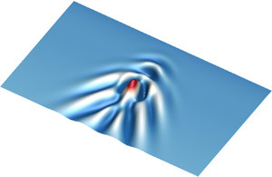
The DNS was performed on a flat plate at Ma 3. A turbulent spot was generated by introducing a localized disturbance on the wall surface near the leading edge. Figure 10 shows the development of a turbulent spot from a linear wave packet until nonlinear breakdown. Time has been normalized by length 1 mm and free stream velocity. At $t=180$, the wave packet transports within a linear region, which is initiated by a small point disturbance. Due to instability of the boundary layer, the wave packet becomes 3-D (labelled $A$). The first-mode wave transports fastest as an oblique wave, and the second-mode wave is not important in this case. By $t=270$, the wave packet has travelled farther downstream, is of a larger amplitude (labelled $B$), undergoes a nonlinear growth, and is close to breakdown. The wave packet propagates in both lateral and streamwise directions. As the wave packet becomes more unstable, the rear wave grows more 3-D, like a $\varLambda$ structure (see the stage at $x\approx 250$). By $t=360$, the wave packet amplitude has grown to a point of unstable breakdown (labelled $C$). Following the breakdown, a turbulent spot develops as an arrowhead-shaped structure. The shape of the spot is consistent with the typical structure described by Krishnan & Sandham (Reference Krishnan and Sandham2006) and others.

Figure 10. Turbulent spot development using isosurfaces of $\lambda _2$ criteria at non-dimensional times $t=180,270,360$ at Ma 3(from left to right), $\lambda _2 = -0.001$.

4.2. Timelines and material surfaces

To examine the details of the spot development, timelines are initiated in $x=182$ and $x=270$ to illustrate the timeline patterns within the linear and nonlinear regions. Figure 11(a) shows the evolution of the wave packet within an early linear region (see supplementary movie 1 available at https://doi.org/10.1017/jfm.2020.1023 for the complete evolution). The colour of the points indicates the wall-normal distance. There are two wave fold structures (labelled $B$ and $C$), with an HSL forming between the two waves. As a result, fewer particles are present in this position, e.g. at the centre of the wave packet $z=60$, a ‘bubble-free heart-shaped’ region (labelled $H$) appears at $x=220\text{--}235$ due to the HSL. The ‘heart-shaped’ region caused by a sequential wave folds is analogous to the hydrogen bubble visualizations shown in Acarlar & Smith (Reference Acarlar and Smith1987a) that are caused by the induced flow of two sequential hairpin heads. In the region between $x=202\text{--}214$, timelines show a high-speed streak (HSS) developing on the centreline, accompanied by two tilted LSS to either side of the centreline. The HSS just follows an LSS caused by the wave fold $B$, which creates a squeezing effect at position $x=216$. Another wave fold is generated at this location, which causes the wave packet to grow in the streamwise direction.

Figure 11. Timelines of wave packet development within the linear and nonlinear regions: (a) timelines initiated within the linear region at $x=182$, (b) timelines initiated within the nonlinear region at $x=270$. (See the supplementary movies 1 and 2 for the complete evolution.)

The nonlinear development of the wave packet is shown in figure 11(b), which is close to the breakdown region. Here, the timelines are initiated at $x=270$ and $z=42\text{--}74$. An apparent $\varLambda$-vortex is observed in the middle of the packet, which causes particles to roll up near the location of the hairpin legs. Two LSS appear at the rear of the wave packet, which looks markedly similar to conventional LSS observed in a turbulent boundary layer. However, these LSS are clearly observed to develop from a weak wave structure (region labelled $A$ in figure 11a), and not from the presence of vortices. The particles between the two wave folds move toward the edges between the LSS and HSS, where an HSL develops (see supplementary movie 2 for the complete evolution).

Figure 12 shows the evolution of material surfaces in proximity to the spot at different wall-normal distances, i.e. $y=2.4$ and $y=0.98$. The contour colours (with contour lines) show the distance from the wall surface. Within the upper material surface at $y=2.4$, the influence of the spot appears as a pair of oblique waves due to the 3-D instability. During the development, an apparent 3-D wave appears within the middle of the packet (labelled $A$). For the material surface initiated at $y=0.98$, 3-D waves also form close to the wall, labelled as $B$ in figure 12(b). By $t$ = 224, figure 12(c) shows that for the material sheet at $y=0.98$ three 3-D waves align into a streamwise pattern, which has the appearance of an LSS. This pattern is similar to the O-regime transition in Jiang et al. (Reference Jiang, Lee, Chen, Smith and Linden2020a).

Figure 12. The evolution of material surfaces initiated at $y = 0.98$ and 2.5: (a) $t = 194$; (b) $t = 209$; (c) $t = 224$. (See the supplementary movie 3 for the complete evolution.)

4.3. LAE contours within the turbulent spot

Figure 13 shows the LAE for the turbulent spot, integrated from time $t=180$ to $t=270$. Figure 13(a) shows an isosurface of $LAE_{180}^{270}=20 \ {\rm s}^{-1}$, coloured with wall-normal distance. The upper layer at $y\approx 1.8$ reveals a pattern of oblique waves, which is consistent with the upper material surface pattern of figure 12. Figure 13(b) shows an isosurface of $LAE_{180}^{270}=26\ {\rm s}^{-1}$, which appears as three parts. The first part (labelled $A$) is a near-wall structure. This part distributes laterally due to the transverse vorticity which is large near the wall surface. However, the head of structure $A$ shows a streamwise concentration of enstrophy, which is associated with LSS within the near-wall region, whose presence were shown previously in figure 12(c). The second part (labelled $B$) is a $\varLambda$-shaped structure, which is at a wall-normal distance $y\approx 1.5$. The nearby fluid particles rotate around the centreline of the legs of a $\varLambda$-vortex, which agrees with the behaviours of timeline particles in figure 11. The third part (labelled $C$) shows two streamwise vortices in front of the $\varLambda$-shaped structure, with the mechanism for their formation being unclear.

Figure 13. The LAE ($\textrm {LAE}_{180}^{270}$) for a turbulent spot: (a) 3-D isosurfaces of LAE ($\textrm {LAE} = 20$), coloured with wall-normal position; (b) 3-D isosurfaces of LAE ($\textrm {LAE} = 26$); (c) contours of LAE in $x$–$y$ plane at $z = 65$; (d) contours of LAE in $z$–$y$ plane at $x = 163$. The same colourbar applies for panels (c) and (d).

Figure 13(c) shows the contours of LAE in the $x$–$y$ plane at $z=65$, as there is no special structure on the centreline $z=60$. The main LAE contours concentrate at $y\approx 1.0\sim 1.5$ (labelled $D$), which is consistent with the $\varLambda$-vortex structure shown by figure 13(b). The contour lines are weakly inclined at a small angle in the streamwise direction, which means the $\varLambda$-vortex has a weak lift-up influence on the nearby fluid particles. An apparent interface is observed at $y\approx 1.7$, appearing as a wave-like undulation. This interface separates the strong mixing zone ($D$) from the non-mixing zone (N). Figure 13(d) shows the LAE contours in the $z$–$y$ plane at $x=163$. The structure labelled $E$ is one leg of a $\varLambda$-vortex, while the hump structure near the wall surface (labelled $F$) is an LSS formed by 3-D waves, as was also shown by figure 12(c).

5.1. Description of data set

The experimental data set used in this study was obtained using tomographic particle image velocimetry (Tomo-PIV), which is the same as Jiang et al. (Reference Jiang, Lee, Smith, Chen and Linden2020b). A brief introduction of the experiment is given here. The experiment was performed in the Peking University water tunnel (PUWT), which is an open-surface recirculating water channel with a cross-section of $0.4\ \textrm {m} \times 0.4\ \textrm {m}$ and length of 6 m. The tunnel free stream velocity range is from 0.1 to $1.3\ \textrm {m} \ \textrm {s}^{-1}$, with a turbulence level of $0.77\,\%$ for tunnel velocities of 0.1 to $0.3\ \textrm {m} \ \textrm {s}^{-1}$. The plate has a chord length of 1.8 m, a span of 0.8 m and a thickness of 15 mm. The flat plate was mounted vertically on the centreline of the tunnel at zero angle of attack. A trailing flap was mounted at the end of the plate to introduce circulation and thus adjust the stagnation point on the leading edge. There would be a separation bubble at the tip of leading edge without using a flap. Adjusting the trailing flap to a suitable angle caused early boundary layer transition to turbulence at $x\approx 400\ \textrm {mm}$. This is similar to using a trip wire to initiate transition. Hydrogen-bubble timelines visualization was used to monitor the flow state during the adjustment process, starting from a laminar flow. The angle of the flap was gradually reduced until intermittent flows with random LSS began to appear in the hydrogen bubble pattern.

The free stream velocity employed for Tomo-PIV was approximately $0.17\ \textrm {m} \ \textrm {s}^{-1}$, and the distance, $x_d$, from leading edge to the centre of the measurement region was 502 mm. The Tomo-PIV configuration is shown in figure 14. Four high-speed cameras (Photron FASTCAM SA4) with a resolution of 1024$\times$1024 pixels were used, in a cross-configuration arrangement. The cameras are fitted with Nikon lenses of 200 mm focal length. The Tomo-PIV sampling frequency was 500 Hz, i.e. time increments $\Delta t^{+}\approx$ 0.42 viscous time units. Illumination was provided by a high-speed laser generator from Beijing ZK Laser, DCQ-30Q, a single-cavity double-pulse laser system with a beam wavelength of 527 nm. The four camera/laser system was synchronized using a LaVision's PTU timing controller. The mean diameter of the tracing particles is $11\ \mathrm {\mu }\textrm {m}$. Experiments were conducted at a particle image density of 0.098 particles per pixel.

Figure 14. Experimental set-up for Tomo-PIV (Jiang et al. Reference Jiang, Lee, Smith, Chen and Linden2020b).

Volume self-calibration (Wieneke Reference Wieneke2008) was used on the preprocessed particle images. Volume reconstruction was achieved by sequential motion tracking enhancement (known as SMTE) (Lynch & Scarano Reference Lynch and Scarano2015). The reconstructed volume was $1041 \times 1048 \times 187$ voxels. A multipass approach of four steps was carried out for the volume correlation, and the interrogation volume size for the final pass was $16 \times 16 \times 16$ voxels with a $75 \%$ overlap. The spatial resolution was 12.52 wall units, with grid spacing of 3.13 wall units. As a final step, a Gaussian smoothing filter of $3 \times 3 \times 3$ subvolume (2.3 wall units) was applied to the velocity data. Proper orthogonal decomposition analysis was finally applied to the smoothed velocity data sets, and the first four leading-order proper orthogonal decomposition modes are extracted for noise removal and the extraction of higher modes (Wu Reference Wu2014; Deng et al. Reference Deng, Pan, Wang and He2018).

Based on 3400 frames of velocity field obtained from the Tomo-PIV data at a sampling rate of 500 Hz, the mean turbulent boundary layer velocity profile obtained from the Tomo-PIV data is shown in figure 15, compared with a universally fitted curve for turbulent boundary layers according to the model of Musker (Reference Musker1979). The friction velocity is obtained by fitting the curve of Musker (Reference Musker1979) to the experimental data. An iterative optimization procedure based on a gradient descent algorithm was used for the fitting process. The result gives an average of $u_{\tau } = 0.0104\ \textrm {m} \ \textrm {s}^{-1}$, with a root mean square variation of $1.77 \times 10^{-4}$, as shown in figure 15(b). The average friction velocity was used to normalize the coordinate and time parameters in this study.

Figure 15. (a) Turbulent boundary layer mean velocity profile plotted on log–linear coordinates (Jiang et al. Reference Jiang, Lee, Smith, Chen and Linden2020b). Fitting curves using model of Musker (Reference Musker1979): $\kappa = 0.41$; $B = 5.0$. (b) Variation of friction velocity calculated by fitting the mean velocity profile. Here $x^{*}$ is the physical streamwise distance relative to the calibration centre of the Tomo-PIV measurement.

5.2. Flow visualization

Figure 16 shows plan-view timeline patterns for LSS. The LSS were identified by tracing the peak of the timelines with a narrow or elongated retardation region, as was identified in the literature (Kline et al. Reference Kline, Reynolds, Schraub and Runstadler1967; Kim, Kline & Reynolds Reference Kim, Kline and Reynolds1971; Smith & Metzler Reference Smith and Metzler1983). The plan-view timelines were generated at $y^{+}$ = 27. The figure shows that the timelines, which flank the low-speed region, appear to temporally intersect and crimp, as shown in the regions labelled $A$ and $B$ in figure 16, which appear similar to the pattern labelled LSS1 in figure 11(b). Figure 16 also illustrates two phenomena: (i) the locations of the LSS are adjacent to the locations of higher wall-normal position; and (ii) the flank of the LSS is usually the most unstable region that initiates the breakdown of the LSS pattern, by attracting or repelling neighbour particles.

Figure 16. Timelines initiated at $y^{+} = 27$ at $t^{+} = 0$. The colour contours indicate the wall-normal position of the timeline surface.

In order to further assess 3-D behaviour of an LSS in a turbulent boundary layer and its relationship to a 3-D wave and hairpin vortices, the LSS in figure 16 was further examined. Figure 17 is an oblique view of the development of vertical material sheets initiated in the $z$–$y$ plane at $x^{+} = -416$ from $t^{+} = 0\text {--}32$ at time intervals of $t^{+}=8$. These 3-D representations of the material sheet evolution (within a cross-section) show clearly that near-wall fluid moves upward (labelled L) in a region of an LSS, flanked by the movement of outer region fluid downward at the sides of the streak (labelled S), as indicated by the yellow arrows. As shown in figure 17, as time progresses the fluid in the LSS regions (e.g. regions labelled $L1, L2, L3$) develops into bulge structures at a downstream position (labelled $A, B, C$), creating apparent inflectional profiles, which is analogous to the typical bursting behaviour observed by Kim et al. (Reference Kim, Kline and Reynolds1971). The inflectional region moves away from the wall, creating the same type of kinking behaviour observed in the hydrogen bubble visualizations of Hama & Nutant (Reference Hama and Nutant1963). According to simulations of early (Jiang et al. Reference Jiang, Lee, Chen, Smith and Linden2020a) and late (Zhao et al. Reference Zhao, Yang and Chen2016) transitional flow, a bulge is present before the development of hairpin-like structures, which indicates the bulges may be 3-D structures within the boundary layer. In the region labelled $C$ in figure 17 (corresponding to the $A$ region in figure 16), a bulge appears to rotate at the flanking boundaries (labelled R) and begins to roll up into what is interpreted as counter-rotating streamwise vortices.

Figure 17. Temporal evolution of vertical material sheets in $z$–$y$ plane initiated at $x^{+} = -416$ from $t^{+} = 0\text {--}32$. Vertical material sheets in the $z$–$y$ plane are released at time intervals of $t^{+}=8$.

The evolution of $x$–$z$ material surfaces, initiated at a series of $y$ locations, and spanning the region $-133 <z^{+}< 74$ where LSS appear, is shown in figure 18. As illustrated, these surfaces undergo significant transverse warping, revealing substantial spanwise variations. The evolution of the ‘peak-valley’ patterns reflected by the deformation of the initially planar material surfaces shows strong movement upward, away from the wall, revealing a lift-up behaviour (labelled $L1$ and $L2$), which is consistent with the behaviour of the vertical material surfaces shown in figure 17. The lift-up behaviour initiates near the wall, and progressively develops a 3-D wave-like pattern. Note that two new kinks appear to the sides of the two main peaks within the near-wall region (indicated by arrows labelled $L3$ and $L4$ on figure 18c), which destabilize the LSS, indicating the flank of LSS is most unstable.

Figure 18. Evolution of material surface initiated at $y^{+}$ = 22, 32, 42, 52 and 62: (a) $t^{+} = 0$; (b) $t^{+} = 20$; (c) end-view of panel (b). The initial range of the surfaces: $-133 <z^{+}< 74$; $-372 <x^{+}< -74$.

5.3. LAE contours within the turbulent boundary layer

Figure 19 shows $\textrm {LAE}$ contours in the $x$–$z$ and $z$–$y$ planes, and the identified Lagrangian vortex boundaries via isosurfaces of $\textrm {LAE}$, in the region adjacent to the location of LSS. Two integral intervals with the same time span were applied in computing LAE, i.e. $t^{+} = [0, 40]$ and $t^{+} = [10, 50]$. Figures 19(a) and 19(b) are contours of $\textrm {LAE}_{0}^{40}$ at $y^{+} = 17$ and $x^{+} = 104$, respectively, with isosurface of $\textrm {LAE}_0^{40}= 4500\ {\rm s}^{-1}$ being superimposed on figure 19(a). Two apparent vortices are detected at $z^{+}\approx 65$ and $z^{+}\approx 100$, which are located to either side of the $L2$ of figure 18. The vortex core to the right (marked $B$ in figure 19a) is almost twice the LAE value as that of vortex core $A$. This means that the vorticity is more concentrated on the right-hand side of the streak. Note that vorticity concentrations in regions labelled $C$ and $D$ in figure 19(b) are considered to be weak, which is closely related to the lift-up of streak $L1$ of figure 18(c).

Figure 19. Contour of LAE in a turbulent boundary layer: (a) contours of $\textrm {LAE}_0^{40}$ at $y^{+} = 17$, superimposed with an isosurface of $\textrm {LAE}_0^{40} = 4500\ {\rm s}^{-1}$; (b) end-view contours of $\textrm {LAE}_0^{40}$ at $x = 104$; (c) contours of $\textrm {LAE}_{10}^{50}$ at $y^{+} = 17$, superimposed with an isosurface of $\textrm {LAE}_0^{40} = 4500\ {\rm s}^{-1}$; (d) end-view contours of $LAE_{10}^{50}$ at $x^{+} = 104$.

Figures 19(c) and 19(d) show the contours of $\textrm {LAE}_{10}^{50}$ for the same planes as figures 19(a) and 19(b), taken $\Delta t^{+}$ =10 after figures 19(a) and 19(b). The streamwise structures shown in figure 19(c) are isosurfaces of $\textrm {LAE}_{10}^{50} = 4500\ {\rm s}^{-1}$, which evolve from the main structures shown in figure 19(a), though with some deviation from their previous locations. A comparison of figures 19(a) and 19(c) suggests a persistence and dominance of the right vortex $B$ after $\Delta t^{+}$ = 10, which may explain the new lift-up of $L4$ in figure 18(c) and the rotation $C$ in figure 17. Two LAE concentration regions in figure 19(c), labelled $C$ and $D$ at $z^{+}\approx -156$ and $z^{+}\approx -83$, seem to develop from the weaker regions within the dashed circles in figure 19(b). Note that regions $D$ and $E$ develop on the left and right flanks of the LSS labelled $L1$ in figures 17 and 18.

The 3-D evaluation of the tomographic timelines demonstrates that the LSS is closely associated with 3-D wave behaviour (figure 16), which is similar to the pattern shown for the transitional boundary layer (figure 5) and bypass transition (figure 11). The spatio-temporal deformation of an advected material surface (figure 18) also reveals a 3-D wave behaviour of the LSS, with the subsequent breakdown resulting in ejections and sweeps associated with the bursting process. The quasi-streamwise vortices detected using 3-D LAE criteria shown in figure 19, are identified as the roll up occurring at the high shear interface of 3-D waves on a streak, which are hypothesized to be generated by the amplification and breakdown of the 3-D wave behaviour of the LSS.