


1. Introduction
Since being proposed in 1940s, the scramjet has become the heart of the air breath propulsion system for the air breath hypersonic vehicle (Segal Reference Segal2009). In a scramjet, the hypersonic inlet is an important component that compresses the incoming flow and provides it to the combustion chamber with suitable pressure and velocity. However, due to the immature design technique, as well as the discrepancy between the ground experiment conditions and the actual flight conditions and inlet unstart is inevitable in an operating hypersonic inlet (Tan, Sun & Yin Reference Tan, Sun and Yin2009). The inlet unstart may not only bring structural damage to the inlet and the engine (Voland et al. Reference Voland, Auslender, Smart, Roudakov, Semenov and Kopchenov1999; Zheng, Yan & Zhao Reference Zheng, Yan and Zhao2020; Bagheri et al. Reference Bagheri, Mirjalily, Oloomi and Salimpour2021), but also make the combustion chamber work abnormally and even flameout (Zheng et al. Reference Zheng, Yan and Zhao2020; Sethuraman, Kim & Kim Reference Sethuraman, Kim and Kim2021). Over the past decades, many flight test failures were ascribed to the inlet unstart, including the NASA flight test (Rodriguez Reference Rodriguez2003) and the X-51A flight tests (Lewis Reference Lewis2010).
For this, the hypersonic inlet unstart has been widely investigated numerically and experimentally in the last decades, and there have been some detailed reviews on the characteristics and mechanisms of the unstart flow (Chang et al. Reference Chang, Li, Xu, Bao and Yu2017; Im & Do Reference Im and Do2018). In general, inlet unstart is considered to be the result of multiple factors including the internal contraction ratio (ICR) (Sakata et al. Reference Sakata, Yanagi, Murakami, Shindo, Honami, Shizawa, Sakamoto, Shiraishi and Omi1993; Devaraj et al. Reference Devaraj, Jutur, Rao, Jagadeesh and Anavardham2021), backpressure (Tan et al. Reference Tan, Li, Wen and Zhang2011; Chen & Tan Reference Chen and Tan2019) and the local Mach number (Yuan & Liang Reference Yuan and Liang2006; Hillier Reference Hillier2007). For ICR-induced inlet unstart, Devaraj et al. investigated the local unstart of a hypersonic inlet at Mach 6 using proper orthogonal decomposition and dynamic mode decomposition (DMD) for a better understanding of the unstart phenomenon (Devaraj et al. Reference Devaraj, Jutur, Rao, Jagadeesh and Anavardham2021). Another research about ICR-induced local unstart was carried out by Jin et al., they experimentally studied the high-frequency and broadband-frequency characteristics of the oscillation in unstart flow caused by a large ICR (Jin et al. Reference Jin, Zhang, Tan, Li, Sun and Wang2022). For the inlet of a turbine-based combined-cycle engine, Li et al. investigated its restart/unstart characteristics in detail and summarized the influences of the mode transition and backpressure on the hysteresis behaviour (Li et al. Reference Li, Chang, Jiang, Yu, Bao, Song and Jiao2018). Yu experimentally studied the inlet unstart under different Mach numbers and successfully captured the typical flow structures of inlet start/unstart flows (Yu et al. Reference Yu, Xu, Li, Liu and Zhang2018). Also, Tan et al. first discussed the oscillating flow caused by the downstream mass flow chocking by experiment at a Mach number of 5. The results indicated that unstart will make inlet performance reduce abruptly due to the shock wave system oscillations and the prominent pressure fluctuations. Further, they classified the oscillatory unstart flows into two types, which are ‘little buzz’ and ‘big buzz’ (Tan et al. Reference Tan, Sun and Yin2009). Owing to the researchers’ efforts, the unstart mechanism of a two-dimensional inlet and sidewall compression inlet is considered to be well understood. However, the three-dimensional inward-turning inlet, which consists of complex compression surfaces leading to more complex flow structures and phenomena, still poses great challenges for its application.
In comparison with the canonical hypersonic inlet, the three-dimensional inward-turning inlet with a cross-sectional shape transition to an elliptical throat is more feasible to be used in combination with an elliptical combustor. It is superior to a rectangular cross-section in terms of the structural weight required to support a specified pressure and the wetted area needed to enclose a specified flow area (Smart Reference Smart1999). Correspondingly, the rectangular-to-elliptical shape transition (REST) gives the inlet a large ICR and wetted area. In practice, the inlet in a combined-cycle engine should operate under the off-design condition before being accelerated to the cruise point. Operating at such a low Mach number, especially for the REST inlet with a large ICR, will lead to inlet unstart in all probability and even result in engine flameout (Tan et al. Reference Tan, Sun and Yin2009). More importantly, for an accelerating scramjet that must operate at high Mach numbers, the mode transitions must be accomplished smoothly, and the impacts on the overall acceleration of the engine should be minimized (Rohde Reference Rohde1992). However, most of the efforts for previous studies are concentrated on the mechanism under the design point of the inlet, only a few of them are put into the unstart flow under the off-design condition. Smart and Trexler investigated the start performance of a REST inlet under the off-design condition at a Mach number below its design point by experiment (Smart & Trexler Reference Smart and Trexler2004). Their study revealed that the REST inlet is a viable configuration for vehicles operating over a wide Mach number range, but the inlet will fall into unstart at off-design conditions without appropriate boundary-layer conditioning. Zveginstsev also proved that the flow in the engine duct becomes extremely complicated in off-design modes of inlet operation, which can lead to unpredictable consequences, in particular, to inlet unstart (Zvegintsev Reference Zvegintsev2017). Li et al. proposed a tomography-like flow visualization and realized the sliced visualization of the internal flow of the REST inlet (Yiming, Zhufei & Zhang Reference Yiming, Zhufei and Zhang2021). However, it is still unable to achieve experimental study well for the microscopic flow structure and the interferences between flow structures. Liu et al. and Yu et al., respectively, investigated the hypersonic internal flow under off-design conditions and the basic characteristics of the unstart flow are summarized (Liu, Liang & Wang Reference Liu, Liang and Wang2016; Yu et al. Reference Yu, Xu, Li, Liu and Zhang2018). Furthermore, Johnson et al. studied the inlet designed for Mach 5.5 based on the stream-tracing technology at the off-design condition at Mach 4 (Johnson et al. Reference Johnson, Jenquin, McCready, Narayanaswamy and Edwards2023). Their results are the same as those of Smart (Smart & Trexler Reference Smart and Trexler2004); the inlet could not start without any flow control strategies. Therefore, the inlet unstart phenomenon under off-design conditions should be considered and more efforts are required to understand the mechanism of the REST inlet unstart flow, especially the transitional condition.
From previous studies, the REST inlet unstart flow under the transitional condition, i.e. a specific off-design condition, is a typical self-sustained shock wave–boundary-layer interaction (SWBLI) system with significant low-frequency unsteady features (Li et al. Reference Li, Chang, Yu, Bao and Song2017). In terms of the low-frequency unsteady mechanisms of SWBLI systems, considerable studies were carried out in the canonical two-dimensional SWBLI configurations, including the incident (impinging–reflecting) shock (Ganapathisubramani, Clemens & Dolling Reference Ganapathisubramani, Clemens and Dolling2007), compression ramp (Grilli, Hickel & Adams Reference Grilli, Hickel and Adams2013; Pasquariello, Hickel & Adams Reference Pasquariello, Hickel and Adams2017) and backward-facing step (BFS) and forward-facing step (Hu, Hickel & Van Oudheusden Reference Hu, Hickel and Van Oudheusden2019, Reference Hu, Hickel and Van Oudheusden2020, Reference Hu, Hickel and Van Oudheusden2021). In all the cases, the SWBLI is accompanied by unsteady motions at frequencies that are one or two orders lower than the boundary-layer characteristic frequency (Touber & Sandham Reference Touber and Sandham2009, Reference Touber and Sandham2011). Therefore, tracing the source of this low-frequency unsteadiness is of particular interest. For the two-dimensional inlet and sidewall compression inlet, the SWBLI within these configurations can be simplified into canonical two-dimensional SWBLI cases and their unsteady mechanism is to be well understood. However, the complex flow structures, a series of shock waves, expansion and vortices within the internal flow of the REST inlet, still pose great challenges for the unsteady mechanism explosion of the REST inlet unstart flow. In the current study, we tend to investigate the low-frequency unsteady mechanism in the unstart flow on the REST inlet under its off-design condition. It is beneficial to the better understanding of the inlet unstart phenomenon and helps the design of flow control strategies and the development of an integrated design technology for the REST inlet with a forebody. Moreover, the investigation of the low-frequency unsteadiness mechanism of the REST inlet is also a good supplement to the current SWBLI theories. In this study, the unstart phenomenon of a hypersonic inlet with REST under the off-design operating condition is numerically studied by adopting delay detached eddy simulation (DDES). The unsteady dynamics, especially the low-frequency characteristic of the REST inlet unstart flow, as well as the self-sustaining mechanism of the unstart flow, are investigated. By comparing with the canonical SWBLI configurations, the differences and connections between the low-frequency unsteadiness characteristics in the REST inlet unstart flow and the canonical configurations, and the internal flow mechanism of the inlet unstart flow, are presented. The key conclusions of these unsteady flow phenomena are promising to help a better understanding of the REST inlet unstart and guide the design of effective unstart flow control methods.
The organization of the paper is as follows. The numerical method and detailed computational set-up are given in § 2. Thereafter, the flow patterns of the mean flow and instantaneous flow are summarized in § 3. Also, the characteristic frequencies of the significant unsteady motion are analysed using spectral analysis and the dominating modes in the unstart flow are extracted via three-dimensional DMD. Finally, to characterize the low-frequency evolution of the unstart flow, a physical mechanism of the unsteady REST inlet unstart flow is proposed in § 4. The conclusions of the main results are presented in § 5.
2. Methodology
2.1. Delay detached eddy simulation
The basic governing equations are the Reynolds-averaged Navier–Stokes (RANS) equations. For the additional Reynolds stress in the RANS equations, researchers have constructed many turbulence models to solve it. The shear-stress transport (SST) turbulence model proposed by Menter (Reference Menter1994) is adopted in the current study.
The two-equation SST DDES method is implemented by modifying the dissipation-rate term of the turbulent kinetic energy transport equation as follows:
 $$\begin{gather} \frac{\partial(\rho k)}{\partial t}+\frac{\partial\left(\rho U_i k\right)}{\partial x_i}=\tilde{P}_k-\frac{\rho k^{3 / 2}}{l_{{hybrid }}}+\frac{\partial}{\partial x_i}\left[\left(\mu+\sigma_k \mu_t\right) \frac{\partial k}{\partial x_i}\right], \end{gather}$$
 $$\begin{gather}\frac{\partial(\rho \omega)}{\partial t}+\frac{\partial\left(\rho U_i k\right)}{\partial x_i}=\frac{\gamma}{v_t} \tilde{P}_k-\beta \rho \omega^2+\frac{\partial}{\partial x_i}\left[\left(\mu+\sigma_\omega \mu_t\right) \frac{\partial \omega}{\partial x_i}\right] +2\left(1-F_1\right) \rho \frac{\sigma_{\omega 2}}{\omega} \frac{\partial k}{\partial x_i} \frac{\partial \omega}{\partial x_i}, \end{gather}$$
where  $\rho$ is the density, $\mu$ is the viscosity, $\gamma$ is the specific heat ratio, $\sigma _k$ and $\sigma _w$ are diffusion coefficients of $k$ and $\omega$, $P_k$ is the production term of turbulent kinetic energy, k and $\omega$ represent the turbulent kinetic energy and specific dissipation rate, respectively, $\beta$ is a constant and its value is recommended as 0.09 by Menter (Reference Menter1994). Additionally, $l_{hybrid}$ is the length scale and is defined as
 $$\begin{gather} l_{hybrid}=\min \left\{l_{RANS}, l_{LES}\right\}, \end{gather}$$
 $$\begin{gather}l_{R A N S}=\frac{k^{1 / 2}}{\beta \omega}, \quad l_{L E S}=C_{D E S} \varDelta=C_{D E S} \max \left\{\varDelta_x, \varDelta_y, \varDelta_z\right\}, \end{gather}$$
where  $l_{RANS}$ and $l_{LES}$ are the length scales of the RANS turbulence model and the large eddy simulation (LES) method. Here, $\delta$ is the grid scale, which is equal to the maximum grid spacing in the $x$,
$x$,  $y$ and $z$ directions for the structured grid and $C_{DES}$ is an empirical constant that needs to be calibrated and verified, reflecting the degree of dissipation in different computational fluid dynamics codes. For the SST turbulence model, $C_{DES} = (1-F_1)C^{outer}_{DES} + F_{1}C^{inner}_{DES}$, where $C^{outer}_{DES}=0.61$, $C^{inner}_{DES}=0.78$ and $F_1$ is the internal function in the SST turbulence model (Spalart et al. Reference Spalart, Deck, Shur, Squires, Strelets and Travin2006).
Furthermore, within the DES method exists modelled-stress depletion, which will produce the grid-induced separation. For this, Spalart et al. proposed a new method, named DDES, by constructing a delayed function (Spalart et al. Reference Spalart, Deck, Shur, Squires, Strelets and Travin2006). The length scale of DDES can be expressed as follows:
 \begin{equation} \left. \begin{gathered} \displaystyle l_{hybrid}=l_{R A N S}-f_d \max \left\{0, l_{R A N S}-l_{L E S}\right\} \\ \displaystyle f_d=1 - \tanh \left[\left(8 r_d\right)^3\right] \\ \displaystyle r_d=\frac{v+v_t}{\sqrt{u_{i, j} u_{i, j}} \kappa^2 d^2} \end{gathered}\right\}, \end{equation}
where  $f_d$ is the delayed function, $\mu _t$ is the kinematic eddy viscosity, $\mu$ is the molecular viscosity, $u_{i,j}$ are the velocity gradients, $\kappa$ is the Kármán constant of 0.41 and $d$ is the distance to the wall. A more detailed introduction of the delayed function and the meaning of the parameters can be found in Spalart et al. (Reference Spalart, Deck, Shur, Squires, Strelets and Travin2006).
2.2. Dynamic mode decomposition
We follow the method of Rowley et al. (Reference Rowley, Mezić, Bagheri, Schlatter and Henningson2009) and Schmid (Reference Schmid2010) to perform DMD (also referred to as Koopman mode decomposition) of the three-dimensional flow field. We take  $m+1$ snapshots of three velocity components at each spatial location and express the last snapshot as a linear combination of the previous snapshots. The size of each $x_i$ is the number of grid points multiplied by the number of velocity components. Let $K$ represent a matrix of the different snapshots from $x_0$ to $x_{m-1}$
 \begin{equation} K=\left[x_0, x_1, x_2, \ldots, x_{m-1}\right]. \end{equation}
 Suppose each snapshot  $(x_i)$ is obtained from the application of a linear matrix $A$ to the previous snapshot $(x_{i-1})$
 \begin{equation} K=\left[x_0, Ax_0, A^2x_0, \ldots, A^{n-1}x_0\right]. \end{equation}
 Now, expressing the last snapshot  $(x_m)$ as a linear combination of the previous snapshots
 \begin{equation} x_m=c_0 x_0+c_1 x_1+c_2 x_2+\cdots+c_{m-1} x_{m-1}+r=K c+r. \end{equation}
 In the above equation,  $r$ represents the residual of the linear combination. If the residual is zero, then the above representation would be exact. Here, $C$ is given by
 \begin{equation} c=\left(c_0, c_1, c_2, \ldots, c_{m-1}\right). \end{equation}
 The vector  $c$ is obtained by solving the least-squares problem in (2.6) using singular value decomposition. Based on the above definitions, we obtain
 \begin{equation} AK=K C+r e^t, \quad e^t=(0, 0, \ldots,1), \end{equation}
where  $C$ is a companion matrix whose eigenvalues approximate those of the matrix $A$, which represents the dynamics of the flow. The imaginary part of the eigenvalue gives the frequency while the real part gives the growth rate of the mode. The eigenvector $(\nu )$ or the spatial variation of the DMD mode is obtained from the eigenvector of the companion matrix $(C)$ and the matrix $(K)$. The energy of each DMD mode is the $L2-norm$ of the eigenvector $\nu$. Here, the vectors $x_i$ are obtained by the operation of the nonlinear Navier–Stokes operator and the eigenvalues and eigenvectors approximate the Koopman modes of the dynamical system. Further theoretical and implementation details can be obtained in Rowley et al. (Reference Rowley, Mezić, Bagheri, Schlatter and Henningson2009) and Schmid (Reference Schmid2010).
2.3. Model and grid
The inlet model adopted in the current study is a typical REST inlet designed by a streamline tracing technology for hypersonic flight at a Mach of 6. The free-stream flow parameters in the design condition are shown in table 1. The surface geometry and detailed measurements are provided in figure 1. Also, the definition of the coordinate origin and axis system is marked in figure 1, in which the location of the inlet leading edge is  $( 16\ \textrm {mm} , 0 )$. The model is a total of $1756\ \textrm {mm}$ in length, measured from the leading edge of the compression surfaces to the aft of the isolator. The capture width is $75\ \textrm {mm}$, measured between the leading edge of each sidewall, and the capture height is $306\ \textrm {mm}$ with a total geometric contraction ratio of 6.98 and an ICR of 1.25. The cowl closure occurs 876 mm downstream from the leading edge ( $80\,\%$ of compression surfaces’ length). In addition, REST inlets are usually designed for a specific flight Mach number with an assumed forebody precompression. The current inlet is assumed to be integrated into a vehicle with a planar forebody with $4^{\circ }$ of attack. Therefore, a planar forebody is located in front of the leading edge, which is 480 mm in length and with an angle of $4^{\circ }$.
Table 1. Flow conditions for the REST inlet at the design operating condition.


Figure 1. Side and front views of the REST inlet geometry.
Figure 2 displays the schematics of the computation domain and boundary conditions for the simulations, in which the grid is coarsened by a factor of 4 for clarity. A multi-block structured grid with  $1.3 \times 10^7$ cells is utilized and the grids are refined near the leading edge and body wall. To ensure that the boundary layers, shock interactions and separation zones are resolved properly, the grid is refined in the near-wall region along the normal direction. The first grid spacing from the wall is chosen to ensure that $y+ < 1$. The grid blends smoothly from very high grid density around the leading edge and wall surfaces to coarser grid space in the free-stream region where the flow is smooth. During the simulation, all the outer boundaries are set to be far field, except for the exit planes, which have applied supersonic outflow. All the wall surfaces are no slip and the wall is adiabatic.

Figure 2. Sketch of inlet computational grid. (a) Overview of the grid. (b) Zoom-in view near the cowl-closure leading edge. (c) Zoom-in view near the sidewall leading edge. (d) Zoom-in view near the throat.
2.4. Computational details
In this study, all the numerical simulations are performed by an in-house three-dimensional finite volume solver developed by the authors. This solver has been successfully applied to considerable numerical studies on both supersonic and hypersonic flows (Qu & Sun Reference Qu and Sun2017; Sun, Qu & Yan Reference Sun, Qu and Yan2018; Qu et al. Reference Qu, Chen, Sun, Bai and Zuo2019; Sun et al. Reference Sun, Qu, Liu, Yao and Bai2021; Wang et al. Reference Wang, Qu, Zhao and Bai2022, Reference Wang, Qu, Sun and Bai2023), in which it reasonably captured the complex shock structures and vortical flows. The code solves the three-dimensional compressible Navier–Stokes equations using the detached eddy simulation method coupled with the two-equation SST turbulence model. A Roe flux-difference upwind scheme with a fifth-order weighted essentially non-oscillatory scheme (Liu, Osher & Chan Reference Liu, Osher and Chan1994) flux limiter is employed because of their low numerical dissipation and advantage in flow structure capturing, such as supersonic mixing layer flow, SWBLI region and so on. The state equation for an ideal gas is used, the molecular viscosity is assumed to obey Sutherland's law and the ratio of specific heat  $\gamma$ is 1.4. Detailed free-stream flow parameters at the transitional operating condition are provided in table 2.
Table 2. Flow conditions for the REST inlet at the off-design operating condition.

In order to accelerate the evolution of the unsteady motions for unstart flow, all the DDES simulations are carried out based on the converged steady RANS solutions. Thereafter, the unsteady DDES simulations are performed and a fixed physical time step of  $3\times 10^{-4}\ \textrm {s}$ is employed. In order to ensure the residual at each physical time step is reduced by at least 2–3 orders, 50 subiterations are used for each physical time step. The first 100 000 time steps (corresponding to a physical time period of 30 s) are used to obtain a basic unsteady flow. The subsequent 50 000 time steps (corresponding to a physical time period of 15 s), which contain roughly 16 cycles of the global motion, are employed to obtain the averaged flow and the instantaneous flows used in the following analyses. Figure 3 presents the time-averaged results of the root mean square of the $U$ velocity fluctuation for specific probe positions obtained by different averaging periods (0–4, 0–8, 0–16). From figure 3, the time-averaged results obtained from 8 cycles and 16 cycles show excellent consistency, which is the same for the other parameters of the present simulation. Therefore, it can be considered that the simulation time for the current case is long enough and the effects of initial conditions are negligible.

Figure 3. Root mean square of  $U$ velocity fluctuations in time-averaged flow obtained by different averaging periods.
2.5. Code validation and grid sensitivity
2.5.1. Code validation
In an operating hypersonic inlet, there are always intense SWBLIs and interactions between shock waves. Further, when the engine is operating over a wide range of conditions, the flow inside the inlet changes drastically, which makes the flow patterns more complex (Tan, Sun & Huang Reference Tan, Sun and Huang2012; Qin et al. Reference Qin, Chang, Jiao and Bao2015; Xu et al. Reference Xu, Chang, Zhou and Yu2016; Li et al. Reference Li, Chang, Yu, Bao and Song2017; Huang et al. Reference Huang, Tan, Sun and Wang2018). Therefore, the solver is required to simulate the inlet flow with high accuracy around the SWBLI region.
To check the validity of the numerical method adopted in the current study, the solver is validated by comparing the numerical solution with the experimental result of a typical three-dimensional crossing shock interaction model in Kussoy & Horstman (Reference Kussoy and Horstman1992). The validation model consists of two sharp fins fastened to a flat plate. The oblique shock waves, generated by the fins, intersect each other and interact with the flat plate turbulent boundary layer. Figures 4 and 5 display the geometric parameters, grid distribution and numerical set-up of the validation model. In the experiment, a weak oblique shock wave is induced by the boundary layer at the flat plate leading edge, causing a slight increase in the downstream wall pressure. To eliminate its effect, the free-stream parameters are diagnosed at  $3\ \textrm {cm}$ ahead of the double fins, which has a Mach number $Ma_{\infty }=8.23$ and Reynolds number $Re_{\delta 0}=1.7 \times 10^5$ based on the local boundary-layer thickness $\delta _0=3.25\ \textrm {cm}$. The other free-stream flow parameters are the same as the experimental set-up, as shown in table 3, and the numerical strategy is the same as that in § 2.4.

Figure 4. Geometric parameters and coordinate system of the validation model. The wedge angle for the double fins is  $\alpha = 15^{\circ }$. The arrow indicates the free-stream flows from the leading of the flat plate toward the double fins. The leading edges of the flat plate and the double fins are sharp, and the model is symmetric to the plane $z=0\ \textrm {mm}$ (Kussoy & Horstman Reference Kussoy and Horstman1992).

Figure 5. Sketch of the computational geometry and grid for the double-fin simulation. (a) Overview of the computational geometry. (b–d) Zoom-in views of the grid distributions.
Table 3. Free-stream flow parameters for double-fin simulation.

From all the computational results shown in figures 6 and 7, the comparison between the computed and experimental wall pressure distributions shows good agreement, indicating that the location and strength of the shock interactions and shock wave–boundary-layer interactions are well captured. Furthermore, the yaw angle is exported from the results, which is defined by  $\tan ^{-1}(w/u)$, where $w$ and $u$ are the velocities in the $z$ (spanwise) and $x$ (streamwise) directions, respectively, as shown in figure 8. The yaw angle represents the local direction of the velocity vector in a plane parallel to the flat plate. From figure 8, the computed yaw angle results show good agreement with the experimental values, indicating that the Flow structures are captured with high accuracy by the solver.

Figure 6. Experimental and computed wall pressure at the centre line of the double-fin configuration.

Figure 7. Experimental and computed wall pressure at (a)  $x/\delta _{\infty } = 5.6$, (b) $x / \delta _{\infty } = 6.92$, (c) $x / \delta _{\infty } = 8.31$.

Figure 8. Experimental and computed yaw angle profiles at (a)  $x / \delta _{\infty } = 5.6$, (b) $x / \delta _{\infty } = 6.92$, (c) $x / \delta _{\infty } = 8.31$.
In addition to the double-fin configuration, another configuration with strong unsteady characteristics is adopted to verify the numerical method adopted in the current study. The configuration is an open backward-facing step (BFS) with a supersonic inflow (Hu et al. Reference Hu, Hickel and Van Oudheusden2019, Reference Hu, Hickel and Van Oudheusden2020, Reference Hu, Hickel and Van Oudheusden2021), a sketch of which is shown in figure 9. The supersonic inflow is characterized by the free-stream Mach number  $Ma_{\infty }=1.7$ and the Reynolds number $Re_{\delta _0}=13 718$ based on the inlet boundary-layer thickness $\delta _0$ and the free-stream values for velocity $u_{\infty }$ and viscosity $\mu _{\infty }$. The detailed free-stream flow parameters are shown in table 4. The size of the computational domain corresponds to $[Lx, Ly, Lz]=[110\delta _0, 33\delta _0, 16\delta _0]$, including a length of $40\delta _0$ upstream of the step. The DDES simulation is conducted based on the converged steady RANS solution. Thereafter, a fixed time step of $3\times 10^{-7}\ \textrm {s}$ is used for the calculation, and $20$ subiterations are required to ensure the residual at each physical time step reduces by at least two orders of magnitude. The first 40 000 time steps are employed to establish a statistically stationary state, and then statistics are gathered for the additional 10 000 time steps.

Figure 9. Sketch of the computational domains and grid for backward-facing step simulation.
Table 4. Free-stream flow parameters for backward-facing step simulation.

Figure 10 presents the comparison of the computed distribution and the reference values of the typical parameters along the centre line including the skin friction, the wall pressure and the root mean square of the wall pressure fluctuation. In addition, the  $U$ velocity profile of several positions is provided in figure 11. The results are in good agreement with the reference results. In the separated region and the shear layer, the solver utilized in the current study keeps high solution accuracy.

Figure 10. Experimental and computed results for BFS configuration of (a) skin friction, (b) wall pressure distribution and (c) root mean square of wall pressure fluctuation.

Figure 11. Experimental and computed  $U$ velocity profiles at (a) $x / \delta _0 = 5$, (b) $x / \delta _0 = 10$, (c) $x / \delta _0 = 15$, (d) $x / \delta _0 = 20$.
In summary of the validation cases, the numerical approach adopted in the present study appropriately describes the flow field including the incident shock, the reflected shock and the SWBLI region as well as the separation bubble.
2.5.2. Grid sensitivity
In the current study, two different mesh sizes were adopted to validate the grid independence of the solution. The coarse mesh contains a total of  $9.6 \ million$ grids, and the fine mesh contains a total of $13.2 \ million$ grids. The diagrams of the computational meshes of the whole computational domain are provided in figure 2. To ensure an accurate solution in the boundary layer, SWBLI region and the separated region, the grids are refined near the wall and the region where complex flow structures are generated. The first grid spacing from the wall is set to ensure that $y+ < 1$.
Figure 12(a) displays the time-averaged flows for the slice at the throat for both the fine and coarse grids. Also, the  $U$ velocity profiles of specific probe points obtained by both two grids are provided in figure 12(b). From the results, the $U$ velocity profiles and the flow fields obtained by the two meshes show good agreement and the two meshes demonstrate good grid independence. Furthermore, to obtain more convincing DDES results, the grid size should be small enough to resolve the desired turbulent structures. In the current study, the smallest Kolmogorov scale $\eta = (\nu ^3 / \epsilon )^{1/4}$ is estimated to be approximately $0.08\ \textrm {mm}$ in the SWBLI region and the shear layer. Here, $\nu$ and $\epsilon$ are the kinematic viscosity, obtained according to Sutherland's law, and the turbulent kinetic energy dissipation rate, estimated by the re-normalization group (RNG) $k-\epsilon$ model. In the fine grid used in this study, the grid spacing around the SWBLI regions and the shear layer in $(x, y, z)$ directions are specified to be $(1.0, 0.6, 0.5)\ \textrm {mm}$, which are $(12.5, 7.5, 6.25)$ times the smallest Kolmogorov scale. In summary, the fine grid is considered to be fine enough to resolve the desired flow structures and will be adopted in the present investigations.

Figure 12. Time-averaged results obtained by coarse grid and fine grid; (a)  $U$ velocity contours at the throat, (b) $U$ velocity profiles at probe the points; $x=100\ \textrm {mm}$, $x=300\ \textrm {mm}$, $x=500\ \textrm {mm}$, $x=700\ \textrm {mm}$, $x=800\ \textrm {mm}$.
3. Results and discussion
3.1. Mean flow features
Figures 13 and 14 provide the overall view of the main flow topology of the averaged flow. With the free-stream flow passing the inlet leading edge, a ramp shock is generated by the planar forebody. After the planar forebody, a large-scale separation bubble is located on the compression wall. The overall profile of the bubble is visualized in figure 14 by the iso-surface of  $u=0$ and the maximum thickness of the bubble is $\delta _{max}=46.5\ \textrm {mm}$ observed at $x=736.5\ \textrm {mm}$. The separation point is located at $x=11.1\ \textrm {mm} \sim 30.0\ \textrm {mm}$ and the separation shock wave is oriented at an angle of $\eta =19.3^{\circ } \sim 20.2^{\circ }$. In other words, the separation point is more forward at the further spanwise position and the shock angle is smaller.

Figure 13. Density contours of the time- and spanwise-averaged flow field for slice  $z=0$. The white dashed and solid lines denote the isolines of $Ma=1.0$ and $\partial P / \partial X = 25$. The black dashed and solid lines signify isolines of $u=0$ and $u/u_{\infty } = 0.99$.

Figure 14. Separation bubble of time-averaged flow filed visualized by iso-surfaces of  $u=0$, coloured by the separation bubble thickness. A numerical schlieren at $z=0$ slice is also included.
Figures 15 and 16 display the wall pressure distribution of the inlet model and specific sampling lines with different spanwise positions. Also, the selection of sampling lines is shown in figure 15. From the results, the pressure on the compression wall of different sampling lines shows more similarity compared with the lower wall. To ensure high-efficiency flow compression, the curvature of the compression wall is smaller, leading to a similar wall pressure distribution. At  $x=11.1\ \textrm {mm} \sim 30.0\ \textrm {mm}$, the flow experiences a slight pressure increase on passing through the separation shock. At $x=1105.1\ \textrm {mm}$, an obvious pressure drop can be observed due to the expansive fan induced by the shape transition near the throat. Because of the expansive fan, the skin friction is lower near the throat compared with that of the region beside the throat.

Figure 15. Wall pressure distribution and sampling lines of the time-averaged flow field on the upper (marked by  $\# u$) and bottom (marked by $\# b$) walls. Pressure is normalized by the free-stream static pressure. The position of wall pressure probe points is indicated by the red dots.

Figure 16. Time-averaged wall pressure distribution of sampling lines of the time-averaged flow field (a) on the upper and (b) bottom walls and (c) Mach number contours of the time-averaged flow field for slice  $z=0$. Pressure is normalized by the free-stream static pressure.
After the throat, the pressure continuously increases under the influence of serious reflected shock waves. In contrast, the pressure distributions on the lower wall at different spanwise positions show clear differences because of the cowl leading edge with a large swept-back angle and the profile with large curvature. As shown in figure 16(b), a sharp pressure drop and increase appear at  $x=1032.4\ \textrm {mm}$ and $x=1105.1\ \textrm {mm}$, which are caused by the shape trimming to ensure the smooth transition of the three-dimensional compression surface between the internal compression section and isolator. Furthermore, the bump causing a local pressure drop can reduce the pressure increase and thus inhibit the flow separation, which is beneficial for the overall performance of the REST inlet.
3.2. Instantaneous flow organization
From the results, the REST inlet unstart flow is highly unsteady and has significant characteristics of up–downstream coupling. The flow is affected by both the turbulence disturbance of the upstream boundary layer and backpressure caused by the downstream SWBLI simultaneously (Fu, Bose & Moin Reference Fu, Bose and Moin2022). For a better understanding of the flow patterns, the  $Q$ criterion is selected for vortex visualization. The $Q$ criterion is defined as
 \begin{equation} Q=\tfrac{1}{2}\left(\tilde{\varOmega}_{i j i j} \tilde{\varOmega}_{i j}-\tilde{S}_{i j} \tilde{S}_{i j}\right), \end{equation}
where  $\tilde {S}_{i j}=\frac {1}{2}({\partial \tilde {u}_i}/{\partial \tilde {x}_j}+{\partial \tilde {u}_j}/{\partial \tilde {x}_i})$ represents the symmetric part of the velocity gradient tensor while $\tilde {\varOmega }_{i j}=\frac {1}{2}({\partial \tilde {u}_i}/{\partial \tilde {x}_j}-{\partial \tilde {u}_j}/{\partial \tilde {x}_i})$ is the antisymmetric part. In the region where $Q>0$, the rotational rate of fluid is greater than the strain rate, and the flow is dominated by vortex structures.
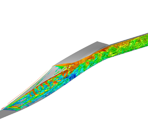
Figure 17 displays the instantaneous flow organization of the computational domains visualized by the iso-surface of  $Q=100$ at $\langle t\rangle =tu_{\infty }/L=8542.1$, time is normalized by the time that the fluid element takes to flow over the whole model with the free-stream velocity. From the results, there is no obvious vortex before the separation point. In contrast, vortical structures are generated over the bubble region. The typical Kelvin–Helmholtz (K–H) vortex structure can be observed near the shear layer and spanwise vortices are generated inside the separation bubble. After the separated region, the vortex structures perform as small-scale arc-shaped vortices affected by the shear layer instability and series of shock interactions. In addition, the arc-shaped vortices of the internal flow are not uniformly distributed but show a cyclical distribution trend along with the reflection of the shock wave in the isolator.

Figure 17. Instantaneous vortical structures at  $tu_{\infty } / L = 8542.1$ visualized by iso-surfaces of $Q=100$, coloured by the streamwise velocity.
Except for the vortex structure, the separation shear layer is another important feature to scrutinize the dynamic motions of the instantaneous flow. Figures 18 and 19 display the streamwise velocity distribution for slice  $z=0$ and the velocity profile at different positions of the symmetry plane. When we take a closer look at the shear layer, there are negative and positive streamwise velocity fluctuations alternating along the shear layer, which is the most typical characteristic of the shear layer.

Figure 18. Contours of the instantaneous streamwise velocity for slice  $z=0$ at $tu_{\infty } / L = 8542.1$. The black arrow lines indicate the streamlines.

Figure 19. Streamwise velocity profile at probe points for slice  $z=0$ at $tu_{\infty } / L = 8542.1$. Streamwise velocity is normalized by the free-stream speed of sound.
In order to illustrate the influence of the compressibility of the fluid on the shear layer, the convective Mach number is proposed and improved by Bogdanoff (Reference Bogdanoff1983) and Papamoschou & Roshko (Reference Papamoschou and Roshko1988). For a mixing layer where two gases on both sides have the same specific heat ratio, the convective Mach number  $M_c$ is defined as
 \begin{equation} M_c=\frac{u_1-u_2}{a_1+a_2}, \end{equation}
where  $u_1$, $u_2$ and $a_1$, $a_2$ represent the flow velocities and local sound speeds for the two streams, respectively. For the supersonic flow, the flow structure of the shear layer is associated with the convective motion of the large-scale structure with the free-stream flow (Papamoschou & Roshko Reference Papamoschou and Roshko1988). Sandham & Reynolds (Reference Sandham and Reynolds1990) proved that the flow structure shows clearly two-dimensional characteristics when $M_c < 0.6$, which is similar to the incompressible flow. In contrast, the shear layer has highly three-dimensional characteristics when $M_c > 0.6$ because of the three-dimensional instability and spanwise unstable waves. Figure 20 shows the vorticity thickness $\delta _w$ and convective Mach number $M_c$ at probe points for slice $z=0$ of the time-averaged flow and the instantaneous flow at $t u_{\infty }/L=8542.1$. The vorticity thickness can be expressed by $\delta _w=\Delta U /|\textrm {d} u / \textrm {d} n|_{max }$, where $\Delta U$ is the difference in velocity of the shear layer and $|\textrm {d} u / \textrm {d} n|_{max }$ is the maximum velocity gradient. From the results, $M_c$ is higher than 0.6 at all the probe points in the separated region. As indicated by Sandham & Reynolds, the compressible shear layer exhibits three-dimensional instabilities at this convective Mach number, which explains the emergence of oblique waves in the shear layer before the impinging point of the cowl-closure leading edge (CLE) shock and shear layer in figure 17. Also, because of the three-dimensional instability, an oblique wave as well as a spanwise flow structure is generated near $x=500\ \textrm {mm}$, causing $\delta _w$ and $M_c$ to decrease, as shown in figure 20. In addition, after the formation of the K–H vortex, $\delta _w$ continuously increases while $M_c$ decreases again at $x=800\ \textrm {mm}$. In the region near the impinging point, the interaction between the shear layer and the shock wave occurs, causing the shear layer instability accompanied by the large-scale vortices being broken into small-scale vortices. As a result, the shear layer after the impinging point seems better mixed and the velocity gradient decreases, causing the increase of vorticity thickness, which is more significant in the instantaneous flow. Alternatively, due to the deceleration after the CLE shock, $u_1-u_2$ decreases after the impinging point, leading to the decrease of convective Mach number at $x=800\ \textrm {mm}$ in figure 20.

Figure 20. Vorticity thickness  $\delta _w$ and convective Mach number $M_c$ at probe points for slice $z=0$ of time-averaged flow and instantaneous flow at $tu_{\infty } / L = 8542.1$.
3.3. Unsteady flow characteristics
As described in the previous subsection, the unstart flow of the REST inlet is highly unsteady. To characterize the regions of most prominent unsteadiness, the variance of the velocity components is provided in figure 21. From the results, taking streamwise Reynolds stress  $\langle u'u'\rangle$ for example, the most active region can be observed along the separated shear layer and after the impinging point, especially in the proximity of the impinging point with a maximum of approximately $1.74u_{\infty }$ at $x=700.9\ \textrm {mm}$, $y=55.5\ \textrm {mm}$, $z=12.5\ \textrm {mm}$. For the other normal Reynolds stress components $\langle v'v'\rangle$ and $\langle w'w'\rangle$, the high-level fluctuation is converged near the aft of the separation bubble, and the maximum of these two components is found further downstream than that of $\langle u'u'\rangle$. These major fluctuations are caused by the instability of the shear layer and separation bubble. The induced shock system and vortex structures enhanced the fluctuations of local flow, leading to the higher normal Reynolds stress. Additionally, relatively weak fluctuations are found along the separation shock, reflecting its unsteady position.

Figure 21. Contours of time-averaged variance of (a) plane at  $z=10\ \textrm {mm}$ and (b) plane at $z=30\ \textrm {mm}$. The black dashed and solid lines denote the isoline of $Ma=1.0$ and $\partial P / \partial X =25$.
Except for these local flow phenomena, large-scale unsteady motion is identified in the unstart flow system. Figure 22 provides the instantaneous velocity field at two instants within a single cycle of the separation bubble motion, which also presents different states, i.e. expansion and shrinking of the bubble. Also, the position of the separation shock (marked as white iso-lines of  $\partial P / \partial X$ ) moves, most notably in the shock foot region. At $t u_{\infty }/L=3006.8$, the separation shock foot is located in the range $x=101.7 \sim 140.8\ \textrm {mm}$ and the shock angle is $\eta =22.9^{\circ } \sim 23.1^{\circ }$. At $t u_{\infty }/L=3228.9$, the separation shock foot is located in the range $x=-0.5 \sim 17.8 \textrm { mm}$, and the shock angle decreases to $\eta =21.1^{\circ } \sim 21.2^{\circ }$. It is clear from this comparison that the recirculation area and separation shock location vary in time. Moreover, the separation bubble thickness at $t u_{\infty }/L=3228.9$ is smaller compared with that at $t u_{\infty }/L=3006.8$. This is because of the increasing interaction between the CLE shock and shear layer as the bubble moves upstream, which accelerates the instability of the shear layer and finally leads to the breaking of the bubble and reduction in the thickness (Zhong et al. Reference Zhong, Qu, Sun, Fu, Wang, Wang and Bai2023).

Figure 22. Contours of the instantaneous streamwise velocity for slice  $z=0\ \textrm {mm}$ and $z=30 \textrm { mm}$ at (a) $tu_{\infty }/L = 3006.8$ and (b) $tu_{\infty }/L = 3228.9$. The black solid line denotes the isoline of $u=0$ and the white solid line signifies the isoline of $\partial P / \partial X =25$.
Figure 23 shows the contours of the instantaneous skin friction coefficient on the compression surfaces at  $t u_{\infty }/L=3006.8$ and $t u_{\infty }/L=3228.9$, corresponding to the instants when the separation point is located at the forefront and rearward position within a single cycle motion, respectively. Also, the outline of the separation bubble is provided by the iso-line of $\langle C_f = 0\rangle$ in figure 23. From the results, distinctly different features can be observed in different regions of the unstart flow. In the upstream region of the flow separation, $\langle C_f = 0\rangle$ is homogeneously distributed. By contrast, clear evidence of the spanwise preferential orientation of the near-wall coherent structures can be observed within the separation bubble. Downstream of the reattachment, streamwise-oriented features can be found, which indicate large-scale streaks with a spanwise alternation of high and low velocity.

Figure 23. Contours of instantaneous skin friction on the compression surfaces at (a)  $tu_{\infty }/L = 3006.8$ and (b) $t u_{\infty }/L = 3228.9$. The solid red line indicates the throat location and the dashed white line indicates the boundary of the separation region ( $\langle C_f \rangle$).
The spanwise alternatively distributed low and high skin friction streaks after the reattachment are believed to be induced by the up-wash and down-wash effects of the streamwise vortices. Figure 24(a) provides the contours of skin friction on the compression surfaces and  $X$-vorticity of specific slices at $t u_{\infty }/L=3228.9$. It should be clarified that the slices in figure 24(a) are converted into rectangular format for a better understanding of the up- and down-wash effects of the streamwise vortices. As shown in figure 24(a) and described in the previous subsection, the near-wall flow after the reattachment is dominated by the streamwise structures with the breaking of the separation bubble. As a result, the wall skin friction between two adjacent streamwise vortices would be enhanced or weakened affected by the down-wash or up-wash effects, as illustrated in figure 24(b). Also, figure 24(c) provides the power spectral density (PSD) of averaged $\langle C_f = 0\rangle$ at three stations at $x=135\ \textrm {mm}$, $x=900\ \textrm {mm}$ and $x=950\ \textrm {mm}$. Downstream of the separation point, i.e. $x=135\ \textrm {mm}$, broadband low-frequency content can be observed, corresponding to the unsteady breathing of the separation bubble. However, the amplitude of this low frequency is very small at the aft of the bubble. Along the streamwise distance, two significant medium frequencies can be identified, of which the higher one is around $St = fd/u_{\infty } = 0.00116$ and the lower one is around $St = fd/u_{\infty } = 0.00084$. The amplitude of these two characteristic medium frequencies increases gradually along the streamwise distance, especially downstream of the attachment.

Figure 24. (a) Contours of instantaneous skin friction on the compression surfaces and  $X$-vorticity of specific slices at $t u_{\infty }/L=3228.9$. The solid white line indicates the boundary of the separation region. (b) Schematic diagram for the up- and down-wash effects of the alternating distributed streamwise vortices. The positive and negative symbols indicate that the region is affected by down-wash and up-wash effects, respectively. (c) Power spectral density of averaged $\langle C_f\rangle$ at $x=135\ \textrm {mm}$, $x=900\ \textrm {mm}$ and $x=950\ \textrm {mm}$.
Moreover, streamwise alternatively distributed low and high skin friction streaks can be found before the reattachment from figure 23, although this pattern is indistinct. It seems to suggest that the flow structures dominating the local flow field are the spanwise flow structures upstream of the reattachment, whereas streamwise flow structures are dominating the local flow field downstream of the reattachment. The dominant spanwise wavelength is  $\lambda _z \approx 0.5h_t$ ( $h_t$ donates the diameter of the throat), which is very close to the dominant streamwise wavelength. From the results, the transition of the characteristic flow structure seems to be an important issue for the REST inlet to maintain a self-sustaining unstart flow. Detailed mechanisms for it will be investigated in the following subsection.
3.4. Spectral analysis
For the further analysis of the unsteady characteristics of the REST inlet under the off-design operating condition, an overview of frequency characteristics for the separated region and the downstream flow structures is provided by the PSD of the wall pressure at selected probe points on the sampling lines in figure 25. Notably, the unsteady characteristics are quantified by the non-dimensional Strouhal number  $St = fd/u_{\infty }$ based on the inlet length and free-stream velocity. The locations of the probe points and the sampling lines have already been introduced in § 3.1. The further downstream in the station, the more high-frequency signals there are and the difference between the upper and the lower walls is gradually decreasing. In the aft of the isolator, the PSDs of the upper and the lower wall are even identical, which is consistent with our previous study (Zhong et al. Reference Zhong, Qu, Sun, Fu, Wang, Wang and Bai2023). The instability of the shear layer and the separation bubble accelerates the averaging process of the downstream flow, leading to the high level similar PSDs at the aft of the isolator.

Figure 25. The PSDs of the wall pressure with the streamwise distance on the upper and lower walls.
When we take a closer look at the upstream stations, the high-frequency characteristics are not obvious, indicating that the flow is dominated by large-scale flow structures including the breathing of the separation bubble and the unsteady movement of the separation shock wave. With the flow developing downstream, a significant increase in the medium-frequency fraction can be observed, where instability of the separated shear layer occurs and the shedding vortices are formed. In a SWBLI system, these medium-frequency motions are proved to be associated with relatively small-scale flow structures, such as the shedding of the shear layer vortices, compared with the low-frequency motions (Hu et al. Reference Hu, Hickel and Van Oudheusden2021). In the current study, the enhanced medium-frequency motions are caused by the instability of the separated shear layer and the induced shedding vortices. After the impinging point of the CLE shock and the shear layer, the shear layer and the separation bubble rapidly becomes unstable and the shedding vortices break into small-scale vortices. As a result, the flow further downstream is dominated by high-frequency motions.
Except for the wall pressure signals, the temporal evolution and corresponding PSD of streamwise velocity within the shear layer at several prove points are shown in figure 26. At the upstream stations, the regularity of streamwise velocity is more obvious. In contrast, a sharp decrease and sharp increase of the streamwise velocity can be observed at downstream stations, and the decrease process takes more time while the increase occurs in a very short time. This phenomenon is corresponding to the formation of the shedding vortices. The instability of the shear layer and the vortex shedding cause the increase and decrease of the separation bubble thickness, causing the decrease and increase of the streamwise velocity, respectively.

Figure 26. Temporal evolution and corresponding PSDs of streamwise velocity within the shear layer at (a)  $x=300\ \textrm {mm}, y=-64\ \textrm {mm}$, (b) $x=700\ \textrm {mm}, y=-201\ \textrm {mm}$, (c) $x=900\ \textrm {mm}, y=-229\ \textrm {mm}$.
In terms of spectral characteristics, the upstream flow is dominated by low-frequency motions. A low-frequency peak in PSD can be observed at  $St = 4.8 \times 10^{-4}$, which is basically fixed at each station. Alternatively, another higher-frequency peak can be observed at $St = 7.6 \sim 8.6 \times 10^{-4}$ and it increases at the downstream locations affected by the instability of the shear layer.
With regard to the global dynamics, the temporal variation of the separation shock angle and the volume of the separation bubble are shown in figure 27. Notably, the shock angle is obtained according to the slope of a segment. The two endpoints of this segment are the mid-point of the intersections between two fixed sampling lines and the isoline of  $\partial {P} / \partial {X}$. As a result, the value of the shock angle is a series of discrete points, causing the values to converge around several certain values, as shown in figure 27(a). However, this approach will affect more the high-frequency characteristics of the data but have less impact on the low-frequency characteristics, which is what we are concentrating on. The same approach is also adopted in Hu et al. (Reference Hu, Hickel and Van Oudheusden2021) when obtaining the shock angle. Therefore, this approach to obtaining the shock angle is considered to be feasible. Another value, the volume of the separation bubble, is defined as the volume of the region within the iso-surface of $u=0$ and the wall. From the results, two frequency peaks, $St = 4.8 \times 10^{-4}$ and $St = 8.4 \times 10^{-4}$, can be identified from the PSD of the separation shock angle. These two characteristic frequencies are the same as those in the previous analysis. Except for these two frequency peaks, a third medium frequency peak $St = 6.7 \times 10^{-4}$ can be observed. In the same way, three frequency peaks, $St = 3.7 \times 10^{-4}$, $St = 6.2 \times 10^{-4}$ and $St = 12.8 \times 10^{-4}$ can be identified from the PSD results of the separation bubble volume. For both the shock angle and the volume of the separation bubble, some extra characteristic frequencies, $St = 6.2 \times 10^{-4}$, $St = 6.7 \times 10^{-4}$ and $St = 12.8 \times 10^{-4}$, can be observed compared with the results shown in figure 26, which seem to be dominated by the instability of the shear layer and the shedding vortices. As explained previously, the subsonic region in the whole computational domain consists of the separation region and the shedding vortices. Moreover, the formation of shedding vortices is usually accompanied by variations in the separation thickness and the separation shock angle. Therefore, these medium-frequency peaks can be considered to be dominated by the instability of the shear layer and shedding vortices. Furthermore, this explained why the second frequency peak in figure 26 increases at downstream stations.

Figure 27. Temporal evolution and corresponding PSD of (a) separation shock angle  $\eta$, (b) volume of separation bubble, (c) mass flow through isolator, (d) total captured mass flow.
Furthermore, the temporal variations of the mass flow through the isolator and the captured mass flow of the inlet are also provided in figure 27. Among them, the captured mass flow can be categorized into two components, one of which is used to sustain the scale of the separation bubble and another goes directly through the isolator. From the results, both the mass flow and the captured mass flow share identical periodicity and mean value, while the captured flow exhibits more periodic and regular fluctuations. This is because the captured mass flow is influenced only by the separation point location and the separation shock angle. Consequently, two frequency peaks,  $St = 6.7 \times 10^{-4}$ and $St = 8.4 \times 10^{-4}$, can be observed in figures 27(c) and 27(d), which are the same as those of the shock angle. In addition to this, $St = 3.7 \times 10^{-4}$, $St = 5.8 \times 10^{-4}$ and two frequency peaks around $St = 12.8 \times 10^{-4}$ can be identified, which are close to the dominant frequency of the separation bubble volume. This finding demonstrates that the mass flow is influenced not only by the movement of the separation point and the flapping motion of the separation shock, but also by the vortex shedding. Furthermore, it explained why the mass flow exhibits higher-frequency characteristics compared with the captured flow, as depicted in figure 27(d). It can be also evidenced by the following coherence analysis of figure 29, where the mass flow and the separation bubble volume demonstrate high coherence in the above frequencies. Upon comparing the mass flow and the total captured mass flow, it is observed that up to $24.18\,\%$ of the captured flow is prevented from entering the isolator because of the maintenance of the separation bubble. For this, the effects of the separation bubble and shear layer instabilities on the flow capture characteristic of the inlet in an unstart flow cannot be disregarded in practical applications.
To confirm the connection between the low- and medium-frequency motions and the flow patterns, several flow parameters are extracted from the current result and statistical analysis is carried out via the coherence  $C_{xy}$ and phase $\theta _{xy}$
 $$\begin{gather} C_{x y}(f)=\left|P_{x y}(f)\right|^2 /\left(P_{x x}(f) P_{y y}(f)\right), \quad 0 \leqslant C_{x y} \leqslant 1, \end{gather}$$
 $$\begin{gather}\theta_{x y}(f)=\operatorname{Im}\left\{P_{x y}(f)\right\} / \operatorname{Re}\left\{P_{x y}(f)\right\}, \quad -{\rm \pi} \leqslant \theta_{x y} \leqslant {\rm \pi}. \end{gather}$$
 In which  $P_{xx}$ is the PSD of $x(t)$, and $P_{xy}$ indicates the cross-PSD between $x(t)$ and $y(t)$. For a certain frequency, the relation between two signals is not linear or there is noise in the datasets if $0 < C_{xy} < 1$. When $C_{xy} = 1$, $x(t)$ and $y(t)$ are linearly related. Conversely, $C_{xy} = 0$ signifies that these two signals are completely unrelated.
The coherences and phases between the separation shock angle and several parameters extracted from the computational domains are provided in figure 28. The definitions of the separation shock angle and the volume of the separation bubble are the same as before. In figure 28(a), two high values of coherence ( $C_{xy} = 0.82$ and $C_{xy} = 0.83$) are observed at the frequencies $St = 7.3 \times 10^{-4}$ and $St = 15.9 \times 10^{-4}$ with large phases of $\theta = 0.679 {\rm \pi}$ and $\theta = 0.798 {\rm \pi}$, which signifies that the shock angle and the separation point are highly related to each other around the dominant low and medium frequencies in figure 27. This is predictable since the shock angle and the separation point are both related to the scale and location of the separation bubble. With the separation bubble moving downstream, the thickness of the separation bubble increases, accompanied by the increases in the shock angle. Also, figures 28(b) and 28(c) indicate that the streamwise velocity within the shear layer and the volume of the bubble are nonlinearly related to the shock angle around the dominant low and medium frequencies. In the same way, the formation of shedding vortices can be reflected by the volume of the separation bubble and the velocity within the shear layer at downstream stations, which has been proven in the previous analysis. Another study of our previous work about the unsteady mechanism for inlet unstart flow at the off-design condition also indicates that the influence of the shedding vortices can propagate upstream within the subsonic region and influence the scale and location of the separation bubble, which will further affect the separation point and shock angle (Zhong et al. Reference Zhong, Qu, Sun, Fu, Wang, Wang and Bai2023). The above observations demonstrate that the unsteady low-frequency behaviour is related to the breathing of the separation bubble and the flapping motion of the separation shock wave, while the medium-frequency motions are associated with the shedding vortices of the shear layer. For this, a decoupling of the frequency scales is required to further trace the sustained source of the intrinsic unsteadiness of inlet unstart flow, which is the objective of the next subsection.

Figure 28. Coherence and phase between separation shock angle  $\eta$ and (a) separation point, (b) streamwise velocity at $x=300\ \textrm {mm}, y=-64\ \textrm {mm}$, (c) volume of the separation bubble.

Figure 29. Coherence and phase between the volume of the separation bubble and mass flow through the isolator.
3.5. Dynamic mode decomposition analysis of the three-dimensional flow field
To better investigate the low-frequency dynamics of the REST inlet unstart flow from the coupled broadband-frequency spectrum, a modal decomposition of the three-dimensional flow field is performed based on DMD. Figure 30(a) displays the eigenvalue spectrum of DMD. From figure 30(a), all the eigenvalues for both pressure fluctuation and  $X$-velocity fluctuation results are distributed near the unit circle, indicating that all the modes decoupled from the unstart flow are quasi-stable modes. This is predictable from the temporal results in §§ 3.3 and 3.4 since each parameter is quasi-periodically distributed in a fully evolved unstart flow.

Figure 30. (a) Eigenvalue spectrum from DMD and (b) mode amplitudes at different frequencies.
From the frequency-magnitude spectrum, a main mode and three characteristic modes are selected from the frequency spectrum based on the analysis above, as shown in table 5. The dominant frequency of the main mode  $\phi _1$ is basically coincident with the dominant frequency of the unstart flow of Trapier's studies (Trapier, Deck & Duveau Reference Trapier, Deck and Duveau2008). Figure 31 displays the real part of the main mode $\phi _1$ with iso-surfaces of the pressure fluctuation at two different phase angles. At these two instants, the prime feature of the modal fluctuation is the structure along the compression waves, including the separation shock, CLE shock and the shock series within the internal flow. Comparing the modal fluctuations at these phase angles, the separation shock continuously exists while the shock series within the internal flow exists intermittently since the internal flow is influenced by the flow structures around the reattachment. As a result, the shock strings make a large contribution to the overall flow only at certain phases. Figure 32(a) gives the modal of pressure fluctuation on the slice $z=0$ in which the effect of shocks and compression waves in mode $\phi _1$ is more clear.
Table 5. Information of the selected modes.


Figure 31. Isosurfaces of the pressure fluctuations from DMD mode  $\phi _1$ with phase angle (a) $\theta = {\rm \pi}/ 2$ and (b) $\theta = 3{\rm \pi} / 4$, only including the real part (red: $p' / p = 0.0003$, blue: $p' / p = -0.0003$).

Figure 32. Real part of DMD mode  $\phi _1$ indicating contours of modal (a) pressure fluctuations and (b) streamwise velocity fluctuations on the slice $z=0$. The black solid line indicates the location of shock wave visualized by isoline of $\partial P / \partial X$ from the mean flow.
Figure 33 gives the modal fluctuation of the streamwise velocity of the main mode  $\phi _1$ at two different phase angles similar to figure 31. Compared with the modal fluctuation of pressure, the key features are centralized around the shear layer and the downstream flow, where active vortices occur. Large fluctuations are streamwise distributed and are mainly distributed around the shear layer and near-wall region, as shown in figure 32(b). Other modes with similar frequency to $\phi _1$ are also examined, the large fluctuations can be observed around the compression waves from DMD of the pressure fluctuation. In the same way, the motion of the shear layer can be observed in the results of streamwise velocity fluctuation, indicating that the separation bubble and separation shock are the most significant flow patterns for the REST inlet unstart flow, as can be seen in figure 21. In addition, an obvious structure can be observed outside the cowl lip, which is caused by the streamwise vertices induced by the spillage around the cowl-closure leading edge. In an experimental study of the inward-turning inlet by Li et al., the same flow structure is also observed by schlieren and this flow structure is proved to have a significant influence on the downstream flow (Yiming et al. Reference Yiming, Zhufei and Zhang2021). However, the spillage and streamwise vertices within the outflow are out of the scope of the current study. Detailed information about it can be found in Yiming et al. (Reference Yiming, Zhufei and Zhang2021), Zhang, Li & Yang (Reference Zhang, Li and Yang2021) and Wang et al. (Reference Wang, Li, Zhang, Liu, Yang and Lu2018).

Figure 33. Isosurfaces of the streamwise velocity fluctuations from DMD mode  $\phi _1$ with phase angle (a) $\theta = {\rm \pi}/ 2$ and (b) $\theta = 3{\rm \pi} / 4$, only including the real part (red: $p' / p = 0.0003$, blue: $p' / p = -0.0003$).
For mode  $\phi _2$, the pressure fluctuations visualized by the isosurfaces are shown in figure 34, in which the fluctuations with high levels are mainly distributed along the CLE shock and shock series around the reattachment. Compared with mode $\phi _1$, the periodicity of the fluctuation is more obvious downstream of the reattachment, indicating that the three-dimensional feature in $\phi _2$ is also stronger than that in $\phi _1$. Large and small fluctuations are alternately distributed in the streamwise direction, revealing a propagation of waves from the impinging point of the shear layer and CLE shock and outwards along the shock waves. From the pressure fluctuations distribution of symmetry in figure 35(a), the radiation of waves along the streamwise and shock can be observed more obviously.

Figure 34. Isosurfaces of the pressure fluctuations from DMD mode  $\phi _2$ with phase angle (a) $\theta = {\rm \pi}/ 2$ and (b) $\theta = {\rm \pi}$, only including the real part (red: $p' / p = 0.0003$, blue: $p' / p = -0.0003$).

Figure 35. Real part of DMD mode  $\phi _2$ indicating contours of modal (a) pressure fluctuations and (b) streamwise velocity fluctuations on the slice $z=0$. The black solid line indicates the location of shock wave visualized by isoline of $\partial P / \partial X$ from the mean flow.
In comparison, the streamwise velocity fluctuations are displayed in figure 36. Smaller-scale vortical structures can be observed compared with  $\phi _1$. These vortical structures are mainly distributed along the streamwise direction and show small periodicity in the spanwise direction. This is because the evolution of the streamwise vortices is limited by the side-wall and compression surfaces, causing the small periodicity in the spanwise direction. Furthermore, the distribution of the streamwise velocity fluctuations shows high similarity to the skin friction distribution on the compression surfaces in figure 24. From the motion of reconstructed flow based on $\phi _2$, the propagation of the disturbance starting from the reattachment of the bubble and the shedding vortices is obvious, indicating that this mode, as well as the low-frequency motion, are associated with the breathing of shock waves and motion of the shear layer.

Figure 36. Isosurfaces of the streamwise velocity fluctuations from DMD mode  $\phi _2$ with phase angle (a) $\theta = {\rm \pi}/ 2$ and (b) $\theta = {\rm \pi}$, only including the real part (red: $p' / p = 0.0003$, blue: $p' / p = -0.0003$).
For the mode  $\phi _3$ with higher dominant frequency, which is associated with the motion of shedding vortices, the pressure fluctuations and streamwise velocity fluctuations are shown in figures 37 and 38. From the results, the pressure fluctuations are centred around the CLE shock wave and the reattachment, indicating that mode $\phi _3$ with higher frequency is related to the motion of shedding vortices. At the same time, the streamwise velocity fluctuations are elongated and distributed in the streamwise direction, which reveals that the motion of shedding vortices is associated with the generation of streamwise structures around the reattachment. Furthermore, the results illustrate that the effect of the CLE shock on the shear layer is to accelerate the instability of the shear layer and thus the shedding vortices are formed. In other words, the CLE shock plays an important role during the dominant flow structure converting from spanwise backflow within the separated region to streamwise vortices around the reattachment, as shown in figures 23 and 24.

Figure 37. Isosurfaces of the streamwise velocity fluctuations from DMD mode  $\phi _3$ with phase angle (a) $\theta = {\rm \pi}/ 2$ and (b) $\theta = {\rm \pi}$, only including the real part (red: $p' / p = 0.0003$, blue: $p' / p = -0.0003$).

Figure 38. Isosurfaces of the streamwise velocity fluctuations from DMD mode  $\phi _4$ with phase angle (a) $\theta = {\rm \pi}/ 2$ and (b) $\theta = {\rm \pi}$, only including the real part (red: $p' / p = 0.0003$, blue: $p' / p = -0.0003$).
4. Physical mechanism of REST inlet unstart flow
In comparison with the traditional two-dimensional or quasi-two-dimensional SWBLI configurations, the flow topology of the REST inlet unstart flow shows significantly different features. In the canonical impinging shock, ramp shock, forward- and backward-facing step cases, the geometry and flow topology are relatively simpler and the separation bubble is induced by only a single oblique shock or the step. Alternatively, the REST inlet consists of irregular compression surfaces generated by a comprehensive consideration of streamline tracking and shape transition rather than the multiple ramps in the two-dimensional case, leading to significant differences in the flow structure in the unstart flow. In REST inlet unstart flow, a large-scale separation bubble is located on the compression surfaces with a separation shock in front of the bubble. Near the maximum thickness of the bubble, a CLE shock induced by the CLE interacts with the shear layer and accelerate the instability of the shear layer. Downstream of the separated region, the flow performs as small-scale arc-shaped vortices affected by the shear layer instability and series of shock interactions.
The instantaneous flow visualized in 3.3 illustrates the localized and global unsteady motion of the REST inlet unstart flow under the off-design condition, which involves the oscillation of separation shock, breathing of the separation bubble, the interaction between the CLE shock and shear layer, instability of the shear layer and the formation of the shedding vortices. Also, the result indicates that the most unstable global mode is mainly distributed around the shear layer and the region where the shedding vortex occurs. The spectral analysis in 3.4 reveals that there are two types of low frequencies around  $St = 4 \times 10^{-4}$ and $St = 7 \times 10^{-4}$, corresponding to the coupling of the breathing bubble and the oscillation of the separation shock. A higher medium frequency is associated with the shedding vortices. These can be also visualized by the streamwise velocity and pressure fluctuation from three-dimensional DMD analysis and the contribution of each selected characteristic mode reveals the contribution of a specific flow structure to the low- and medium-frequency interaction. Apart from the unsteady separation bubble and shedding vortices, the DMD mode also reveals the transition from spanwise-dominated flow to streamwise-dominated flow motion downstream of the separation. In both instantaneous flow and DMD mode, ‘Görtler-like vortices’ are observed. However, the formation and evolution of the Görtler vortices are limited due to the large contraction ratio in the spanwise direction of the REST inlet, thus only a counter-rotating vortex pair (CVP) and seldom small-scale streamwise vortices are formed, as shown in figures 36 and 37. However, the CVP produces a similar effect on the unstart flow. During the whole process when the flow undergoes the localized and global unsteady motions, the separation bubble is required to remain within a certain scale and location. In other words, the shear layer instability and shedding vortices will strip mass from the separation bubble. Therefore, another way in the flow field exists to replenish the mass of the separation bubble opposite to the shedding vortices. From the flow structure and unsteady motion on the unstart flow, it seems that the flow is injected into the separation bubble and becomes part of the backflow inside the bubble affected by the flow structures around the reattachment. Thus, the scale and location of the separation bubble maintain dynamic equilibrium.
We believe that the low- and medium-frequency mode transition is associated with the self-sustaining of the separation bubble. Around the reattachment, the main flow structure converts from spanwise backflow into streamwise vortices, as shown in figures 23 and 24. Affected by the up- and down-wash effects of the CVP, low and high skin friction streaks are formed downstream of the reattachment. Further, the streamwise vortices accelerate the process of downstream flow averaging, causing similar spectral characteristics at downstream stations in figure 25. For the CVP, the mechanism of their generation is displayed in figure 39. As shown in figures 39(b) and 39(c), the shedding vortices are formed and developed centred on symmetry. As a result, the backflow of the shedding vortex produces an up-wash effect on the flow near the wall around the reattachment. Affected by the up-wash effect and spanwise instability of the shear layer, the CVP is formed.

Figure 39. Sketch of the entrainment–injection model sustained by the CVP: (a) contraction process, (b) dilatation process and (c) schematic diagram for up-wash effect of the shedding vortex. The black dashed and blue solid lines signify the flow structure in the averaged flow field and instantaneous flow field.
Estruch-Samper and Chandola proposed an entrainment–recharge mechanism to associate low-frequency unsteadiness with the shedding effects (Estruch-Samper & Chandola Reference Estruch-Samper and Chandola2018). In this theory, the bubble's decay–growth dynamics is associated with the low-frequency mechanism by the shear layer's motion and the Strouhal number of the low-frequency breathing can be related to the entrainment frequency as
 \begin{equation} S t_r^{{low }}={\rm \pi} \alpha_{\varepsilon} \xi_B \delta^{\prime 2} \frac{L_r}{h}\left(X_r^{e n t}\right)^2 S t_r^{e n t} \approx C_{\varepsilon} \frac{L_r}{h}\left(X_r^{e n t}\right)^2 S t_r^{e n t}, \end{equation}
where  $\alpha _{\varepsilon }$ is the length-to-thickness ratio of the shedding coherent structures, $\xi _B$ signifies the percentage of the entrainment mass and $\delta ^{\prime }$ is the spreading rate of the mixing layer. Huang et al. have proved that the difference between these three variables in different cases is small, thus the multiplication of these three parameters can be considered as a constant $C_{\varepsilon } = \alpha _{\varepsilon } \xi _B \delta ^{\prime 2}$. Also, $L_r / h$ is the ratio of the bubble length to bubble height and $X^{ent}_r$ is the non-dimensional entrainment length which depends on the specific geometry and flow pattern. In canonical cases including impinging shock and ramp cases, the entrainment usually only occurs in the rear half of the separation bubble, leading to a non-dimensional entrainment length $X^{ent}_r \approx 0.5$ (Piponniau et al. Reference Piponniau, Dussauge, Debieve and Dupont2009). For the unstart flow of the REST inlet, the instability is affected by the CLE shock at the maximum thickness of the separation bubble. Therefore, the entrainment only occurs after the impinging point of the CLE shock, resulting in an approximate non-dimensional entrainment length $X^{ent}_r \approx 0.15$ and the geometry-dependent transformation factor is $C^{ent}=(X^{ent}_r)^2 {L_r} / {h} \approx 7.7$. The entrainment frequencies $St^{ent}_r$ of these cases are similar, thus the REST inlet unstart flow yields an approximately 5 times larger $St^{ent}_r$ than the impinging shock and ramp cases, and 2.5 times larger $St^{ent}_r$ than the forward- and backward-facing step cases under the same free-stream condition. However, this model only provides an estimate of the low frequency, and an accurate value is not expected to be obtained.
Based on the discussion above, the following physical mechanism is proposed for the low-frequency unsteadiness in the REST inlet unstart flow. The incoming flow undergoes a strong adverse pressure gradient and shear upon separation, leading to large coherent vortical structures along the shear layer. Near the maximum thickness location of the bubble, the shear layer rapidly becomes unstable, which is affected by the CLE shock. correspondingly, the shedding vortices are formed and the mass is entrained as displayed in figure 39(a). Moreover, the streamwise vortices are generated around the reattachment driven by the shedding vortices and centrifugal instability. Under the joint effect of shedding vortices and large-scale streamwise vortices, the mass is injected into the separation bubble, thus the scale and the location of the separation bubble are sustained. Additionally, the consecutive entrainment recharge leads to the breathing of the separation bubble as well as the flapping of the separation shock, as observed from the streamwise velocity fluctuations of the DMD mode in figures 33–37. Therefore, the large-scale vortices and the shedding vortices are the main driving force of the global low-frequency unsteadiness of the REST inlet unstart flow under the off-design condition.
5. Conclusions
Numerical simulation was carried out by DDES to study the unsteady mechanism of the REST inlet unstart flow under the off-design condition at a Mach of 4. With the help of highly accurate numerical simulations, the mechanism of unsteadiness, especially the low-frequency characteristics, is investigated. Compared with the canonical SWBLI cases, the flow topology of the REST inlet unstart flow shows significantly different features since the REST inlet consists of irregular compression surfaces generated by a comprehensive consideration of streamline tracking and shape transition rather than the multiple ramps in the two-dimensional inlet. In the REST inlet unstart flow under the off-design condition, a large-scale separation bubble is located on the compression surfaces with a separation shock in front of the bubble. Near the maximum thickness of the bubble, a CLE shock induced by the CLE interacts with the shear layer and accelerates the instability of the shear layer. Moreover, strong unsteady motion can be observed in the unstart flow, including the breathing of the separation bubble, flapping of the separation shock, interaction between the CLE shock and shear layer, instability of the shear layer and the generation of the shedding vortices. Among them, the most unstable global motion is distributed around the shear layer and the region where the shedding vortex forms.
From the spectral analysis, there is a broad band of low-frequency oscillations in the REST inlet unstart flow. The lower-frequency dynamics is associated with the breathing of the separation bubble and the flapping motion of the separation shock wave, while the higher frequency is related to the instability of the shear layer affected by the CLE shock and the formation of shedding vortices. The phenomena mentioned below have a significant influence on the flow capture characteristic of the unstart inlets. Further, coherence analysis shows that the contributions of these flow structures dominating the low-frequency dynamics are coupling with each other. For this, three-dimensional DMD analysis is carried out to reveal the characteristics that contribute to the observed unsteady behaviour. The large fluctuations observed in mode  $\phi _1$ illustrate that the separation bubble and separation shock are the most significant flow patterns for the REST inlet unstart flow, as can be seen in figure 21. Mode $\phi _2$ provides evidence that low-frequency motion is associated with the breathing of the shock waves and shear layer. Mode $\phi _3$ with higher dominant frequency is related to the motion of shedding vortices. At the same time, the elongated distributed streamwise velocity fluctuations indicate that the generation of the streamwise structures around the reattachment is coupled with the motion of shedding vortices. The streamwise vortices and the shedding vortices are the main driving force of the global low-frequency unsteadiness of the REST inlet unstart flow under the off-design condition. Moreover, the CLE shock plays an important role in the process during the dominant flow structure conversion from the backflow within the separated region into the elongated streamwise structure.
Funding
This study was co-supported by National Natural Science Foundation of China (no. 11902265, no. 11972308) and Natural Science Foundation of Shaanxi Province (no. 2019JQ-376) and the Fundamental Research Funds for the Central Universities (no. G2018KY0304, no. G2018KY0308).
Declaration of interests
The authors report no conflict of interest.
Data availability statement
The data that support the findings of this study are available from the corresponding author upon reasonable request.


