


1. Introduction
The prediction of preferential orientation of anisotropic particles in turbulent flows is of importance because of the many implications it can have for industrial and environmental applications (Voth & Soldati Reference Voth and Soldati2017). Anisotropic particles have applications in industrially relevant flows, such as in pulp and papermaking (Lundell, Söderberg & Alfredsson Reference Lundell, Söderberg and Alfredsson2011) and environmental problems, like modelling of phytoplankton (Guasto, Rusconi & Stocker Reference Guasto, Rusconi and Stocker2012; Basterretxea, Font-Munoz & Tuval Reference Basterretxea, Font-Munoz and Tuval2020), sedimentation (Meiburg & Kneller Reference Meiburg and Kneller2010), aerosols (Kleinstreuer & Feng Reference Kleinstreuer and Feng2013), ice crystals in clouds (Kristjànsson, Edwards & Mitchell Reference Kristjànsson, Edwards and Mitchell2000; Shultz Reference Shultz2018; Jiang et al. Reference Jiang, Verlinde, Clothiaux, Aydin and Schmitt2019) and micro-fibre pollution in oceans (Ross et al. Reference Ross2021). In recent years, significant effort has been devoted to investigating numerically the dynamics of rigid and axisymmetric ellipsoids in homogeneous and isotropic turbulence (HIT) (Shin & Koch Reference Shin and Koch2005; Ni, Ouellette & Voth Reference Ni, Ouellette and Voth2014; Byron et al. Reference Byron, Einarsson, Gustavsson, Voth, Mehlig and Variano2015; Pujara, Voth & Variano Reference Pujara, Voth and Variano2019) and in turbulent channel flow (Mortensen et al. Reference Mortensen, Andersson, Gillissen and Boersma2008; Marchioli, Fantoni & Soldati Reference Marchioli, Fantoni and Soldati2010; Zhao, Marchioli & Andersson Reference Zhao, Marchioli and Andersson2014; Zhao et al. Reference Zhao, Challabotla, Andersson and Variano2015; Challabotla, Zhao & Andersson Reference Challabotla, Zhao and Andersson2015a,Reference Challabotla, Zhao and Anderssonb; Marchioli, Zhao & Andersson Reference Marchioli, Zhao and Andersson2016; Zhao & Andersson Reference Zhao and Andersson2016; Dotto & Marchioli Reference Dotto and Marchioli2019; Dotto, Soldati & Marchioli Reference Dotto, Soldati and Marchioli2020). Natural fibres can have complex and non-regular shapes, difficult to systematically characterise. Therefore, many theoretical and numerical investigations have been focused on axisymmetric ellipsoids: in this case fluid torques are mathematically trackable, and this shape has the advantage that the torques on small particles with many other shapes are the same as their equivalent ellipsoids (Bretherton Reference Bretherton1962; Brenner Reference Brenner1963). Many analyses of axisymmetric ellipsoids in turbulence have been conducted via numerical simulations, but the high computational costs limiting the applications to moderate Reynolds numbers, an exception being the recent numerical simulation of Jie et al. (Reference Jie, Xu, Dawson, Andersson and Zhao2019). The common assumption of these works is that the particle size is set to be smaller than the smallest length scale of the flow, a condition that might not be satisfied in practical applications. Recent numerical investigations of finite-size ellipsoid in turbulent channel flow (Do-Quang et al. Reference Do-Quang, Amberg, Brethouwer and Johansson2014; Eshghinejadfard, Hosseini & Thevenin Reference Eshghinejadfard, Hosseini and Thevenin2017; Wang et al. Reference Wang, Abbas, Yu, Pedrono and Climent2018; Zhu, Yu & Shao Reference Zhu, Yu and Shao2018; Ardekani & Brandt Reference Ardekani and Brandt2019; Zhu et al. Reference Zhu, Yu, Pan and Shao2020) overcame this small-size assumption, but they are limited to even lower flow Reynolds numbers, small overall number of particles and small fibre aspect ratio.
In parallel with numerical works, experimental investigations have also been considered. However, much fewer studies have been provided experimentally. A brief review of experimental works on anisotropic particles is presented in table 1. All investigations consider rigid, anisotropic particles with three planes of symmetry, e.g. rod- and disk-like particles. From table 1, it clearly emerges that a major proportion of the experimental studies in this field is limited to two-dimensional visualisation, and such studies focused mainly on orientation and concentration analysis (Bernstein & Shapiro Reference Bernstein and Shapiro1994; Parsheh, Brown & Aidun Reference Parsheh, Brown and Aidun2005; Dearing et al. Reference Dearing, Campolo, Capone and Soldati2012; Håkansson et al. Reference Håkansson, Kvick, Lundell, Prahl Wittberg and Söderberg2013; Abbasi Hoseini, Lundell & Andersson Reference Abbasi Hoseini, Lundell and Andersson2015; Yang et al. Reference Yang, Francois, Punzmann, Shats and Xia2019). In this context, Capone, Miozzi & Romano (Reference Capone, Miozzi and Romano2017) studied the dynamics of rigid, rod-like particles in turbulent channel flow. They showed that, with respect to the channel centre, the relative fibre concentration decreases linearly within the buffer layer and towards the channel wall without any sign of accumulation in the near-wall region. Di Benedetto, Koseff & Ouellette (Reference Di Benedetto, Koseff and Ouellette2019) investigated the preferential orientation of rod and disk-like particles in a free surface gravity wave flow. Using planar image analysis, the orientation of the particles as a function of the wave strength was studied. They showed that the probability density function (p.d.f.) of the orientation angles has a bimodal distribution due to the opposing forces of wave and settling, and a portion of the particles has the tendency to orient perpendicularly with respect to the wave plane. Recently, Bakhuis et al. (Reference Bakhuis, Mathai, Verschoof, Ezeta, Lohse, Huisman and Sun2019) performed a series of experiments using straight cylinders inside a Taylor–Couette facility in the ultimate turbulence regime. The particle diameter and length were both larger than the Kolmogorov length scale of the flow. Interestingly, they showed that the particle preferential orientation with respect to the inner wall of the Taylor–Couette cell is independent of Reynolds number and particle concentration. Both concentration and orientation can give important insights about the dynamics of the fibres. However, to look at the full rotational dynamics, three-dimensional measurements are required.
Table 1. Summary of experimental investigations of anisotropic particle-laden flows available in the literature. Apparatuses and techniques are reported and abbreviated as follows: pipe flow (PF), orientation density function (ODF), close water loop (CWL), two-dimensional image processing (2D-IP), shallow electrolytic fluid layer (SEFL), two-dimensional phase discrimination (2D-DS), two-dimensional tracking (2D-T), homogeneous isotropic turbulence (HIT), three-dimensional tracking (3D-T), two-dimensional particle image velocimetry (2D-PIV), water table (WT), turbulent pipe jet (TPJ), von Kàrmàn flow (VKF), two-dimensional particle tracking velocimetry (2D-PTV), stereoscopic particle image velocimetry (S-PIV), wall-bounded channel flow (WBCF), cube tank turbulence (CTT), vertical wall-bounded channel flow (VWBCF), Taylor–Couette (TC), surface gravity wave flow (SGWF), Rayleigh–Bénard cell (RBC) and three-dimensional phase discrimination (3D-DS). Here  $\textit {Re}$ is the Reynolds number and [1], [2], [3] and [4] refer to bulk, integral, wall shear and particle Reynolds numbers, respectively. The $\textit {Re}$ in [5] is calculated based on root mean square of velocity. Ratio $\lambda$ refers to aspect ratio of the objects and in [1] and [2] $\lambda$ is measured by considering the arm of the objects. Parameter ${\textit {St}}_{\eta }$ is the particle translational Stokes number, but in works marked as [1] and [2], authors introduced a tumbling Stokes number to evaluate their data. Ratio $L_{f}/l_{{flow}}$ stands for the ratio of the length of the objects to the flow length scale. In the works marked with [1] and [2], $L_{f}$ is calculated by taking to account one arm of the objects, whereas in that marked with [3], equivalent diameter is used.

Volumetric experimental studies of anisotropic particles focused mainly on the rotational dynamics of particles in HIT, as listed in table 1. Parsa et al. (Reference Parsa, Calzavarini, Toschi and Voth2012), for the first time, performed series of experiments in HIT and tracked slender rods with various aspect ratios using a three-dimensional tracking technique. They showed that the orientation of anisotropic and inertialess particles is correlated with the velocity gradient tensor. This behaviour could be different in the presence of a shear flow, where fibres can either align with the vorticity vector or be parallel to the wall, as a result of the balance between mean velocity gradient and fluctuating velocity gradient (Voth & Soldati Reference Voth and Soldati2017). The aim of the present work is to capture the fibre dynamics in conditions of high shear, in the vicinity of the channel wall, and in quasi-shear-free conditions, in the core of the domain, to try to compare our results with those of previous works on HIT. Parsa & Voth (Reference Parsa and Voth2014) reported a scaling law for the mean square rotation rate of rods as a function of the length of fibres in the inertial range, i.e. with particle size larger than the smallest scale of the flow. Following the same approach, a modified scaling for the tumbling rate of rod-like particles was provided in subsequent works by Bordoloi & Variano (Reference Bordoloi and Variano2017), Bounoua, Bouchet & Verhille (Reference Bounoua, Bouchet and Verhille2018), Kuperman, Sabban & van Hout (Reference Kuperman, Sabban and van Hout2019) and Bordoloi, Variano & Verhille (Reference Bordoloi, Variano and Verhille2020). Recently, Jiang, Calzavarini & Sun (Reference Jiang, Calzavarini and Sun2020) investigated the rotation of oblate and prolate spheroids in a Rayleigh–Bénard flow. They showed that the trend of the tumbling rate as a function of the aspect ratio, due to shear, has a peak for weakly oblate spheroids, in contrast with the monotonic universal trend previously reported for HIT configuration. All these works significantly improved the understanding of the dynamics of axisymmetric fibres in turbulent flow. However, in most industrial and environmental applications, rod-like particles are not axisymmetric; they have an asymmetry in their shape or mass distribution. Experimental results for the settling behaviour of inertial rods (Roy et al. Reference Roy, Hamati, Tierney, Koch and Voth2019) showed that rods undergo a critical change in orientation due to asymmetry in their mass distribution, and it was shown theoretically (Hinch & Leal Reference Hinch and Leal1979) and numerically (Wang et al. Reference Wang, Tozzi, Graham and Klingenberg2012; Crowdy Reference Crowdy2016; Thorp & Lister Reference Thorp and Lister2019) that even small deviations from an axisymmetric shape can produce a significant change of the rotational dynamics. To the best of our knowledge, neither experimental nor numerical works on non-axisymmetric shape particles in turbulent flows are currently available, and we aim precisely at filling this gap. Using a novel experimental methodology, we are able to evaluate the effect of curvature on the dynamics of the fibres.
In this study, we investigate the dynamics of long, non-axisymmetric fibres in a turbulent channel flow. Experiments are carried out in the TU Wien Turbulent Water Channel, which is a gravity-driven, large-aspect-ratio facility. Turbulence is naturally generated by a long hydrodynamic developing length. Fibres used in this study are neutrally buoyant, have various curvatures and all are dispersed in the flow simultaneously. Three-dimensional imaging of the fibres is carried out to reconstruct their shape and spatial orientation and to track their motion. The database produced consists of concentration, orientation and rotation rates of fibres that are classified according to their curvature. The measurements cover more than half of the channel height, to capture both the centre of the channel (HIT-like motion) and the near-wall region (inner and buffer layers, controlled by shear and viscous forces). The fibres used in this study can be considered as slender bodies with high length-to-diameter ratio,  $\lambda =120$, and very small Stokes number, ${\textit {St}}=0.003$.
The paper is organised as follows: In § 2, the experimental facility, particle parameters and recording settings are described. The methodology used to reconstruct and track the fibres is presented in § 3. Finally, distribution, orientation and rotation rates of the fibres classified according to their curvature are discussed in §§ 4 and 5.
2. Experimental set-up
We measure experimentally the three-dimensional distribution, orientation and rotation rate of long fibres in a fully developed, turbulent channel flow. In this section, we describe the experimental apparatus, flow parameters, fibre properties and three-dimensional fibre detection technique used in this study.
2.1. Flow apparatus
The experimental facility is the TU Wien Turbulent Water Channel, consisting of a 10 m long water channel, constructed by combining five sections of 2 m each, with cross-sectional dimensions of  $80\ \textrm {cm}\times 8\ \textrm {cm}$ ( $w\times 2h$, where $h$ is half-channel height). Each section of the channel is equipped with de-airing valves, which allows the removal of bubbles trapped close to the top wall of the channel. The channel is manufactured using poly(methyl methacrylate) with a thickness of 1.5 cm, which is fully transparent. The experimental set-up is sketched in figure 1(a). The upper cover of the channel is removable in all sections, and both open- and closed-channel experiments can be performed. In this study, we only consider the closed-channel configuration with no free surface. The fluid is circulated from the downstream to the upstream reservoir by a pump, and the flow is subsequently driven by gravity. A centrifugal volute pump (maximum flow rate of $147\ \textrm {m}^{3}\ \textrm {h}^{-1}$) and a Proline Promag 10D electromagnetic flowmeter are used. Average temperature of the water is kept at $15\,^{\circ }\textrm {C}$, which results in a dynamic viscosity equal to $\mu =1.138\times 10^{-3}\ \textrm {Pa}\ \textrm {s}$ (Korson, Drost-Hansen & Millero Reference Korson, Drost-Hansen and Millero1969). In order to eliminate all vibrations, possibly created by either the pump or the chiller of the laser, both equipments are placed on vibration isolators.

Figure 1. Schematic of the TU Wien Turbulent Water Channel and test section. (a) The system consists of two reservoirs at ambient pressure, a centrifugal pump and a rectangular channel (aspect ratio of 10). The test section is located 8.5 m downstream of the channel entrance, to ensure a fully developed turbulent flow. (b) Close-up view of the test section, where an array of four cameras is used to record the three-dimensional motion of the particles. The laser volume, indicated by the green region, is located at the channel mid-span. To reduce the optical image distortion due to astigmatism, cameras look through prisms filled with water. The laboratory reference frame ( $x,y,z$, respectively streamwise, wall-normal and spanwise directions) is also shown. (c) Field of view of the cameras and illumination volume.
2.2. Flow and fibre properties
In all experiments, a constant flow rate of  $39.6\ \textrm {m}^3\ \textrm {h}^{-1}$ has been chosen, corresponding to a bulk velocity of $0.172\ \textrm {m}\ \textrm {s}^{-1}$ and a bulk Reynolds number based on channel full height ( $2h$) of $\textit {Re}_{b}=12\,500$. The shear velocity of the unladen flow is $u_{\tau }=10.2\ \textrm {mm}\ \textrm {s}^{-1}$, which gives a friction Reynolds number $\textit {Re}_{\tau }=u_{\tau }h/\nu =360$, where $\nu$ is the kinematic viscosity of water at $15\,^{\circ }\textrm {C}$. Viscous time and length scales of the flow are $\tau =\nu$/ $u_{\tau }^2\approx 11$ ms and $\delta =h/\textit {Re}_{\tau }\approx 110\ \mathrm {\mu }\textrm {m}$, respectively. Kolmogorov time and length scales of the flow at the centre of the channel are computed as $t_{\eta }=(\tau ^{2}/\epsilon _{d}^+)^{0.5}\approx 220$ ms and $l_{\eta }=(\delta ^{4}/\epsilon _{d}^+)^{0.25}\approx 500\ \mathrm {\mu }\textrm {m}$, where $\epsilon _{d}^+$ is the turbulent dissipation in wall units obtained from the DNS database.
In this study, the fibres consist of Polyamide 6.6 Precision Cut Flock (Flockan) with linear density of  $\rho _{l}=9\times 10^{-8}\ \textrm {kg}\ \textrm {m}^{-1}$ (0.9 dtex). The density and cutting length are $\rho =1.15\times 10^{3}\ \textrm {kg}\ \textrm {m}^{-3}$ and $L_{f}=1.2$ mm, respectively, corresponding to a diameter $d_{f}=\sqrt {4 \rho _{l}/(\rho {\rm \pi})} \approx 10\ \mathrm {\mu }\text {m}$. In figure 2, we present a microscopic view of the fibres considered in this study. This observation is important because we used this initially qualitative view to categorise the shape of the fibres in a systematic way. In figure 2(a), we show a raw image of a large quantity of the fibres in dry condition. Fibres are very elongated and characterised by a large value of anisotropy ratio $\lambda =L_{f}/d_{f}\approx 120$ and in addition they are characterised by a small curvature. In figure 2(b), we show a limited number of fibres on a white horizontal background. In this view, we can better appreciate the curvature and also, more importantly, we can appreciate that all fibres are planar. Finally, from the close-up view of figure 2(c), fibres seem to present no inflection point. Observing many samples like the ones presented in figure 2 led us to hypothesise that fibres can be described by a second-order polynomial curve. This point together with the methodology used to detect and model the fibres are further discussed in § 3.2. Relative length and diameter of the fibres to the length scales of the flow, $L_{f}/l_{\eta }$, $L_{f}/\delta$, $d_{f}/l_{\eta }$ and $d_{f}/\delta$, are equal to 2.38, 10.58, 0.02 and 0.09, respectively.
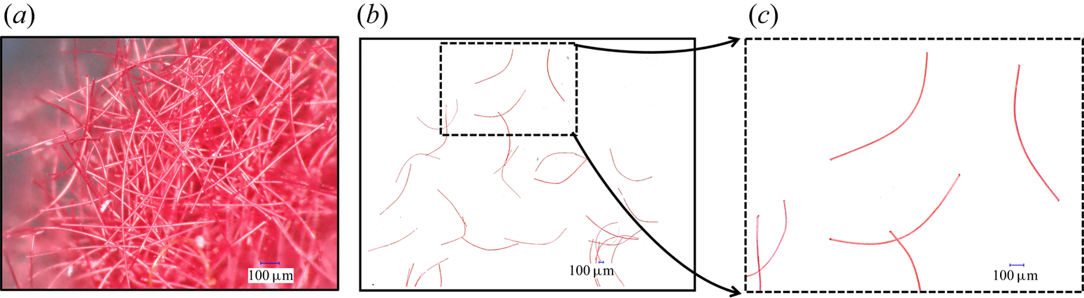
Figure 2. Fibre samples. (a) Raw image of a cluster of fibres (microscope view). (b,c) Close-up view of fibres characterised by different shapes, mainly non-axisymmetric.
The dimensionless parameter used to characterise the behaviour of particles transported by the flow is the particle Stokes number,  ${\textit {St}}$, which quantifies the ratio between the particle relaxation time, $\tau _{f}$, and the viscous time scale, $\tau$. To estimate the translational relaxation time of the fibres, we use the relaxation time of randomly oriented prolate spheroids. We considered the relation proposed by Bernstein & Shapiro (Reference Bernstein and Shapiro1994), which gives
 \begin{equation} \tau_f=\frac{\rho d^{2}}{18\mu}\frac{\lambda \ln \left(\lambda +\sqrt{\lambda^{2}-1}\right)}{\sqrt{\lambda^{2}-1}} { ,} \end{equation}
where  $d$, in the case of anisotropic and axisymmetric particles, is the diameter perpendicular to the symmetry axis. Although fibres used in the present study are not exactly prolate spheroids, (2.1) can provide a good approximation of their relaxation time. The $\tau _{f}$ computed as in (2.1) is based on the relaxation time of a spherical particle $(\rho d^{2}/18\mu )$, and corrected for prolate spheroids as function of the fibre aspect ratio, $\lambda =L_{f}/d_{f}$. In the present study, the relaxation time of the fibres is $\tau _{f}=3.5\ \mathrm {\mu }\textrm {s}$, corresponding to ${\textit {St}}=0.003$. In the centre of channel, the Kolmogorov time scale should be used to estimate the Stokes number rather than viscous time scale. As a result, the particle Stokes number based on the Kolmogorov time scale at the channel centre is $1.54\times 10^{-4}$. We observe that in both cases the Stokes number is small enough to neglect any possible inertial effect.
In the following, we provide an estimate of the maximum deformation that fibres can experience. To this aim, we assume a simplified flow configuration in which a straight fibre is cylindrical, blocked at one end and free to move at the other end (cantilever beam). For simplicity, we consider the flow as uniform, perpendicular to the fibre axis and characterised by a velocity  $u_\tau$. We choose this penalising configuration to show that, also in the presence of critical conditions, the deformation experienced by the fibre is negligible, and that fibres can be considered as rigid objects. We assume that the fibre Young's modulus is $E=2.5$ GPa (i.e. half of that measured for fibres having a diameter of $20\ \mathrm {\mu }\textrm {m}$; Bunsell (Reference Bunsell2001)). The Reynolds number of the fibre $Re_f=u_\tau d_f/\nu \approx 0.09$ gives a drag coefficient $C_D=66.1$ (Tang et al. Reference Tang, Tian, Yan and Yuan2014). As a result, the force acting on the fibre is $F_D=C_D\rho u^2_\tau L_f d_f /2=4.1\times 10^{-8}$ N. The maximum fibre deformation is computed with the Euler–Bernoulli theory for beams as
 \begin{equation} w_M=\frac{qL_f^4}{8EI}=7.2\times10^{{-}3}\ \mathrm{mm}, \end{equation}
where  $I={\rm \pi} d_f^4/64$ and $q=F_D/L_f$ is the hydrodynamic force per unit of fibre length, which we assume to be uniformly distributed along the fibre. The maximum value of deformation obtained is sufficiently small ( $w_M/L_f=0.6\,\%$) to consider fibres as rigid bodies. However, longer and more flexible fibres can exhibit large deformations, potentially producing flow modifications due to an intermittent storage/exchange of energy with the fluid (Allende, Henry & Bec Reference Allende, Henry and Bec2018).
2.3. Three-dimensional imaging
The measurement is carried out in correspondence with the test section, located 8.5 m ( ${\approx }200h$) downstream of the channel entrance, to ensure the fully developed flow condition. The measurement volume (
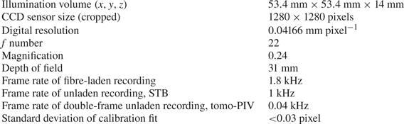
 $53.4\ \textrm {mm}\times 53.4\ \textrm {mm}\times 14\ \textrm {mm}$) is located at the mid-span of the channel. A close-up view of the test section is provided in figure 1(b). Illumination comes from the bottom and consists of a thick laser sheet (527 nm, double cavity, 25 mJ per pulse, Litron LD60-532 PIV). The images are recorded using four Phantom VEO 340 L cameras with sensor size of $2560\times 1600$ pixels at 0.8 kHz and each pixel size is $10\times 10\ \mathrm {\mu }\textrm {m}^2$. The cameras are located on both sides of the channel and in linear configuration. Side and front views of the measurement volume are depicted in figure 1(c). Camera holders are equipped with dampers to remove any possible vibration coming from the channel frame. In order to increase the accuracy of the three-dimensional reconstruction process, we placed the cameras with angles of $35^\circ$ and $30^\circ$ with respect to the spanwise axis of the channel. To minimise the optical astigmatism, we used four prisms filled with water at the side walls of the channel. Finally, the cameras are equipped with Scheimpflug adapters and objective lenses with focal length $f = 100$ mm.
Data acquisition has been performed using three different recording settings for unladen and fibre-laden experiments. The reason behind this choice is the high temporal resolution that fibre-laden experiments require to accurately measure the rotation rate. We used double-frame mode with 3.5 ms time delay for laser pulses for the image acquisition of tomographic particle image velocimetry (tomo-PIV) in the unladen flow. In addition to double-frame recording, to perform 3D-PTV velocimetry in the unladen flow, we recorded single-frame images at 1 kHz acquisition rate. Flow was seeded with tracers, with a diameter of  $20\ \mathrm {\mu }\textrm {m}$, by providing particle-per-pixel concentrations of 0.035 and 0.02 for tomo-PIV and 3D-PTV recordings, respectively (see § 2.4 for further details). Source density number of the recordings, $N_{s}$, which quantifies the total number of pixels occupied by the tracers (for further details, see Scarano (Reference Scarano2012)), is equal to 0.44 for tomo-PIV and 0.25 for 3D-PTV, which fall within the limits recommended by Novara & Scarano (Reference Novara and Scarano2012). In the case of fibre-laden experiments, images have been recorded at 1.8 kHz in single-frame mode, to ensure that the displacement of fibres in the centre of the channel cannot exceed 2 pixels. In this way, the measurements are well resolved in time and the accuracy of the tracking process is higher. Source density number $N_{s}$ in this case is equal to 0.1. Focal length, aperture size and depth of focus were the same for both unladen and fibre-laden recordings and were 100 mm, $f/22$ and 31 mm, respectively (table 2). As a result, the digital resolution of the images is $24.1\ \textrm {pixels}\ \textrm {mm}^{-1}$. The camera sensor size was cropped down to $1280\times 1280$ pixels. Illumination was obtained with the simultaneous emission of both laser cavities.
Table 2. Summary of the camera and laser recording parameters adopted.
Prior to reconstruction of the measurement volume, raw images were preprocessed using time and spatial filters. The first step of image preprocessing consists of removing the background noise by subtracting the minimum intensity value of the dataset from each image. Afterwards, a spatial filter is applied to the images by subtracting the minimum intensity within a kernel of five pixels from each pixel. Finally, the intensities were normalised by the average intensity within a kernel of 300 pixels. These steps were essential for increasing the signal-to-noise ratio of the images and for improving the quality of the reconstruction process. A three-dimensional calibration target with size of  $58\ \textrm {mm}\times 58\ \textrm {mm}$ was used to map the coordinate system of the illuminated volume on the image. Afterwards, a third-order polynomial function was used for the mapping process. Initial standard deviation of the calibration fit was in the scale of 0.3 pixels, which eventually reduced to values smaller than 0.03 pixels (averaged on all camera views) by applying the volume self-calibration (VSC) algorithm (Wieneke Reference Wieneke2008). The VSC was done by assuming $8\times 8\times 5$ ( $x,y,z$) subvolumes and resulted in an average disparity error of approximately 0.02 pixels, which is five times smaller than the recommended threshold for VSC accuracy (Wieneke Reference Wieneke2008). In order to implement the VSC, flow must be seeded with spherical tracers. The multiplicative algebraic reconstruction technique (MART) (Elsinga et al. Reference Elsinga, Scarano, Wieneke and van Oudheusden2006) was used to reconstruct the three-dimensional distribution of light intensity from two-dimensional images of tracer particles and fibres. Since in this study we used MART to reconstruct both unladen and fibre-laden flows and the VSC process was a main step of the calibration to be done before MART, we seeded the water with tracers prior to dispersing the fibres into the water. An example of a raw image of fibre-laden flow containing both fibres and tracer is shown in figure 3. Each snapshot of fibre-laden recording contains, on average, approximately 1000 fibres and the corresponding volume fraction and concentration are $O(10^{-6})$ and $0.025\ \textrm {mm}^{-3}$, respectively. Therefore, it is reasonable to consider that the one-way coupling assumption holds. All processes of image acquisition and single-phase velocimetry have been carried out using Davis (LaVision GmbH).

Figure 3. (a) Example of raw image referring to a portion of the domain. Curved fibres as well as tracer particles can be identified. (b) Close-up view of a group of fibres. The resolution adopted is sufficient to properly characterise the fibres, which consist of tens of pixels.
2.4. Unladen flow velocimetry
The velocimetry of the unladen flow is carried out using both tomo-PIV (Elsinga et al. Reference Elsinga, Scarano, Wieneke and van Oudheusden2006) and shake-the-box (STB) algorithms (Schanz, Gesemann & Schröder Reference Schanz, Gesemann and Schröder2016). The cross-correlation process was applied to interrogation volumes of  $48\times 48\times 48$ voxels. Prior to using the STB method, optical transfer function was applied to correct the shape of particles by fitting an elliptical Gaussian model to each subvolume of the VSC. In total, $3\times 10^4$ tracks in each snapshot were detected by the STB process. To evaluate the properties of the fluid flow considered, we compared single-phase measurements with direct numerical simulations of channel flow at $\textit {Re}_{\tau }=350$. Simulations are based on an in-house pseudo-spectral solver (Fourier–Chebyshev discretisation) (Zonta, Marchioli & Soldati Reference Zonta, Marchioli and Soldati2012). The size of the channel is $4{\rm \pi} h \times 2 h \times 2{\rm \pi} h$ and the domain is discretised with $512\times 513\times 512$ collocation points, in directions $x$,
$x$,  $y$ and $z$, respectively, with the lower wall located at $y=0$. Statistics are computed over a time window of $1500\tau ^{+}$. The mean velocity profile (streamwise) obtained from 3D-PTV (STB) and tomo-PIV is compared with direct numerical simulation results at $\textit {Re}_{\tau }=350$ in figure 4.

Figure 4. Mean velocity profile obtained from 3D-PTV (STB; circles) and tomo-PIV (triangles) compared with direct numerical simulation (DNS) at  $\textit {Re}_{\tau }=350$ (solid line).
3. Fibre detection and tracking
In this study, we use MART to reconstruct the three-dimensional light intensity distribution of both unladen and fibre-laden flows. To discriminate the fibres, we developed a MATLAB-based in-house code, which is described in § 3.1. Fibre modelling is discussed in §§ 3.2 and 3.3. Finally, fibre tracking and calculation of rotation rates are analysed in §§ 3.4 and 3.5, respectively.
3.1. Phase discrimination
The process of fibre discrimination is used to distinguish the fibres from the tracers and other spurious, reconstructed objects, and consists of a combination MART and volumetric masking. An example of the discrimination process is shown in figure 5. First, the three-dimensional light intensity distribution, consisting of normalised intensities (i.e. intensity has values from 0 to 1), is obtained from the MART reconstruction process. The three-dimensional matrix of light intensities is binarised (figure 5a), according to a threshold value set to 0.05. All the groups of contiguous voxels with unitary value are identified as a cluster. Then, an effective length of the cluster  $L_{eff}$, defined in Appendix A, is computed. Finally, clusters with effective length in the range $20<L_{eff}<40$ voxels (red voxels in figure 5(a)) are identified as fibres, and all remaining clusters (blue voxels in figure 5(a)) are removed. The above-mentioned range for the effective length is set by considering the fibre size. By this masking, the majority of the tracers are removed and only large clusters of voxels remain (figure 5b), which mostly represent the real fibres. In some unlikely cases, these clusters may still consist of spurious objects. However, they do not persist over long time periods and can be eliminated by removing the clusters tracked over a short number of snapshots.

Figure 5. (a) Three-dimensional light intensity distribution is obtained using MART (Elsinga et al. Reference Elsinga, Scarano, Wieneke and van Oudheusden2006), and corresponding voxels are shown. (b) After masking, fibres (red voxels) are discriminated from the other objects, e.g. tracers, noise and ghost particles (blue voxels). (c) Close-up view of a small portion of the domain (size is reported). We observe that, although fibres are characterised by a complex shape, they are well captured by the reconstruction and discrimination processes proposed here.
3.2. Fibre modelling
To quantify the fibre concentration, orientation and rotation rate, after discrimination, each fibre has to be associated with the representing coordinates in the three-dimensional space. To this aim, we developed a physically grounded geometrical model for the fibres. We consider a rigid and non-axisymmetric fibre of length  $L_{f}$ and we assume that the fibres are bent but not twisted. This hypothesis is motivated by observations, and represents the ground of the modelling process proposed. As a consequence, one can show that the fibre lies on a plane, i.e. it can always exist in at least one plane, $\varPi$, in the three-dimensional space, $(x,y,z)$, that contains the fibre. An example of voxel distribution, discriminated as in § 3.1, is sketched in figure 6(a), where the colour of the voxels refers to the reconstructed light intensity. The geometrical description of the fibre (red line in figure 6a) is obtained through a process of modelling, consisting of three main steps:
(i) Preliminary determination of the fibre orientation: we consider the cluster of voxels identified as a fibre in the discrimination process. We consider the coordinates of the voxels located at two ends of the fibres and then find the distance between these two points. The direction of the laboratory reference frame $(x,y$ or $z)$ along which this difference is maximum is preliminarily considered as the orientation of the fibre. In figure 6(a), the fibre orientation is $x$, and we define $x$ as the preliminary ‘fibre direction’.
(ii) Identification of the fibre cross-section centres: we consider the light intensities of the voxels defining the fibre. We group the voxels according to the planes perpendicular to the fibre direction. Therefore, each plane represents (approximately) a cross-section of the fibre. We determine the centre of each cross-section as the averaged voxel coordinate (
$x,y,z$) weighted on the light intensity of the voxels. In the fibre shown in figure 6(a), the centres of the cross-sections, $(y,z)$ planes, are found. These centres are explicitly indicated as red stars (figure 6a).(iii) Definition of the fibre major axis: finally, the fibre axis is defined as the best fit of the centres defined above. To this aim, we define the arc length coordinate
$s$, with origin and end in the first and last cross-sectional centres, so that $0\leqslant s \leqslant L_{f}$. To identify the fibre position in space, for each direction $x_{i}$ (where $x_{i}$ stands for $x$, $y$ or $z$), we find the function $f_{x_{i}}$ that best fits in a least-square sense the coordinates of the centres. In this way, the functions $f_{x_{i}}$ required to approximate the fibre coordinate $x_{i}$ as a function of the arc length coordinate $s$ are obtained (figure 6b–d).


Figure 6. (a) Example of fibre reconstruction (red curve) obtained from light intensity distribution. Voxels, here represented as cubes, are coloured according to their light intensity, from lower (white) to higher (black). The laboratory reference frame ( $x,y,z$, blue vectors) is shown, as well as the origin and direction of the arc length coordinate $s$ (green vector), which is used to perform the reconstruction. (b–d) Coordinates of the voxels belonging to the fibres are approximated by three functions ( $\,f_{x},\,f_{y},\,f_{z}$) obtained by fitting the coordinates of the centres, as defined in § 3.2 (red stars in a), as a function of the curvilinear coordinate $s$.
$s$.
In particular, for the present case we set the functions  $f_{x_{i}}$ to be second-order polynomials, so that
 \begin{equation} f_{x_{i}}=a_{i}s^{2}+b_{i}s+c_{i} { .} \end{equation}
One can show analytically that this assumption is consistent with the initial hypothesis that the fibre is contained on a plane. This assumption is also consistent with direct observations of the fibres (see § 2). Indeed, in figure 2(b,c) fibres seem planar and without any inflection point.
The fibre coordinates  $f_{x_{i}}$ can be written in matrix form as
 \begin{equation} {\boldsymbol{x}}_{f}= \left[\begin{array}{@{}c@{}} f_{x} \\ f_{y} \\ f_{z} \end{array} \right] = \left[\begin{array}{@{}ccc@{}} a_{1} & b_{1} & c_{1} \\ a_{2} & b_{2} & c_{2} \\ a_{3} & b_{3} & c_{3} \end{array} \right]\left[ \begin{array}{@{}c@{}} s^{2} \\ s \\ 1 \end{array} \right]= {\boldsymbol{As}} { ,} \end{equation}
where  ${\boldsymbol {x}}_{f}$ is the approximated fibre coordinate vector, ${\boldsymbol {A}}$ is the matrix of the coefficients ( $a_{i}, b_{i}, c_{i}$) and ${\boldsymbol {s}}$ contains the arc length coordinate vector. Therefore, the modelled fibre is fully defined by the matrix ${\boldsymbol {A}}$ and the length $L_f$. An example of the reconstruction process performed for fibres of different shape is shown in figure 7. In particular, we observe in figure 7(a,b) that the fibres (left, red objects taken from microscope images) are well fitted by second-order polynomials (right, black objects obtained from fitting).

Figure 7. Fibre samples. (a–c) Three different classes of fibres, classified according to their curvature, are shown. The fibres (left, red objects taken from microscope images) are well fitted by the second-order polynomials (right, black objects obtained from fitting). This assumption is required to employ the method proposed here.
The proposed fitting method is based on the assumption that the fibre is a parabolic segment. However, even in cases for which fibres are not precisely parabolic segments, like the case shown in figure 7(c), in which fibre curvature exhibits strong gradients, the proposed fitting method supplies a reasonably accurate approximation for the shape of the real fibre.
The next step required for fibre tracking consists of identifying the fibre centre of mass and orientation. We consider now the fibre sketched in red in figure 8(a). The projection of the fibre on the reference planes is shown (blue lines) as well as the centre of mass of the fibre  ${\boldsymbol { G}}=(x_{G},y_{G},z_{G})$, where
 \begin{equation} x_{i,G}=\frac{1}{L_{f}}\int_{0}^{L_{f}}x_{i}(s)\,\text{d}s { ,} \end{equation}
where  $x_{i}$ stands for $x$,
$x$,  $y$ or $z$. The plane $\varPi$ containing the fibre is defined by the equation
 \begin{equation} {\boldsymbol{n}}\boldsymbol{\cdot}\left[{\boldsymbol{e}_{\boldsymbol{1}}}(x-x_{G}) + {\boldsymbol{e}_{\boldsymbol{2}}}(y-y_{G}) + {\boldsymbol{e}_{\boldsymbol{3}}}(z-z_{G})\right] = 0 { ,} \end{equation}
where  ${\boldsymbol {e}_{\boldsymbol {i}}}$ are the unit vectors of the laboratory reference frame and ${\boldsymbol {n}}$ is the unit vector perpendicular to $\varPi$. Given three points of the fibre ( ${\boldsymbol {A}}$, ${\boldsymbol {B}}$ and ${\boldsymbol {C}}$), ${\boldsymbol {n}}$ is determined as
 \begin{equation} {\boldsymbol{ n}}=\left[\begin{array}{@{}c@{}} (y_{B} -y_{A})(z_{C} -z_{A}) - (z_{B} -z_{A})(y_{C} -y_{A})\\ (x_{C} -x_{A})(z_{B} -z_{A}) - (x_{B} -x_{A})(z_{C} -z_{A})\\ (x_{B} -x_{A})(y_{C} -y_{A}) - (y_{B} -y_{A})(x_{C} -x_{A}) \end{array} \right]. \end{equation}
Following Voth & Soldati (Reference Voth and Soldati2017), we define the fibre reference frame using the inertia tensor
 \begin{equation} {\boldsymbol{I}}_{ij}=\rho_{l}\int_{0}^{L_{f}}\left[ (\,f_{x_{i}}-x_{i,G})^{2}\delta_{ij}-(\,f_{x_{i}}-x_{i,G})(\,f_{x_{j}}-x_{j,G}) \right] \text{d}s, \end{equation}
with  $\rho _{l}\ (\textrm {kg}\ \textrm {m}^{-1})$ the linear density of the fibres and $\delta _{ij}$ the Kronecker delta. Therefore, we align the reference frame of the fibre ( $O'x'y'z'$) with the normalised eigenvectors of ${\boldsymbol { I}}$. Note that the eigenvalues of ${\boldsymbol { I}}$ are real and positive and correspond to the principal inertia moments of the fibre, $I_{1}$, $I_{2}$ and $I_{3}$. In the present case, one eigenvalue is much smaller than the other two and we align $x'$ with the corresponding eigenvector. Similarly, $y'$ and $z'$ are aligned with the second and third eigenvector, respectively. When the fibre is curved, $x'$ and $z'$ belong to $\varPi$ whereas $y'$ is aligned with $\boldsymbol {n}$.

Figure 8. (a) Non-axisymmetric fibre (red line) lying on the plane  $\varPi$. The inertial frame of reference, with axes labelled as $x$,
$x$,  $y$ and $z$, remains fixed in space and time. The fibre frame of reference, centred in the fibre midpoint located at $s=L_{f}/2$ ( $O'$, red bullet), has axes ( $x',y',z'$) aligned with the principal directions of the inertia tensor. The projection of the fibre on the three planes is also shown (blue lines). Note that, in general, the centre of mass of the fibre ( $G$, cyan bullet) may be external to the fibre. (b) Angles defined between the reference frame of the fibre ( $O'x'y'z'$) and the reference frame of the laboratory translated to the midpoint $O'$ ( $O''x''y''z''$).
Three angles  $(\vartheta _{x},\vartheta _{y},\vartheta _{z})$ define the relative orientation of the fibre reference frame ( $O'x'y'z'$) with respect to the laboratory reference frame translated to the midpoint of the fibre $(O''x''y''z'')$. The system is represented in figure 8(b). Three rotations (and the corresponding rotation matrices) are required to identify the orientation of the fibre with respect to the laboratory reference frame. To this aim, we use the quaternions formulation (Lecrivain et al. Reference Lecrivain, Grein, Yamamoto, Hampel and Taniguchi2020). We consider the unit vectors of the reference frame $O'x'y'z'$ and $O''x'' y''z''$, respectively $\boldsymbol {e_{1}'},\boldsymbol {e_{2}'},\boldsymbol {e_{3}'}$ and $\boldsymbol {e_{1}''},\boldsymbol {e_{2}''},\boldsymbol {e_{3}''}$. The angle $\vartheta _{x}$ is defined here as the angle required to align $\boldsymbol {e_{1}''}$ with $\boldsymbol {e_{1}'}$. We compute the unit quaternion $\boldsymbol {q}$ as
 \begin{equation} {\boldsymbol{ q}}=\left[ \begin{array}{@{}c@{}} q_{s}\\ q_{x}\\ q_{y}\\ q_{z} \end{array} \right]= \frac{1}{\sqrt{(q_{s}^*)^{2}+(q_{x}^*)^{2}+(q_{y}^*)^{2}+(q_{z}^*)^{2}}} \left[\begin{array}{@{}c@{}} q_{s}^{*}\\ q_{x}^{*}\\ q_{y}^{*}\\ q_{z}^{*} \end{array} \right], \end{equation}
with  $q_{s}^{*}=1+\boldsymbol {e_{1}''}\boldsymbol {\cdot }\boldsymbol {e_{1}'}$ and $[q_{x}^{*}\ q_{y}^{*}\ q_{z}^{*}]^{T}=\boldsymbol {e_{1}''}\times \boldsymbol {e_{1}'}$. The rotation matrix associated with the quaternion $\boldsymbol {q}$ is
 \begin{equation} {\boldsymbol{ R}}_{\vartheta_{x}}=\left[ \begin{array}{@{}ccc@{}} 1/2-q_{y}^{2}-q_{z}^{2} & q_{x}q_{y}-q_{s}q_{z} & q_{x}q_{z}+q_{s}q_{y}\\ q_{x}q_{y}+q_{s}q_{z} & 1/2-q_{x}^{2}-q_{z}^{2} & q_{y}q_{z}-q_{s}q_{x}\\ q_{x}q_{z}-q_{s}q_{y} & q_{y}q_{z}+q_{s}q_{x} & 1/2-q_{x}^{2}-q_{y}^{2} \end{array} \right], \end{equation}
and we have that  $\boldsymbol {e_{1}''}={\boldsymbol { R}}_{\vartheta _{x}}\boldsymbol {e_{1}'}$. The rotation angle is finally determined as
 \begin{equation} \vartheta_{x}=2\text{atan2}\left(\sqrt{q_x^2+q_y^2+q_z^2},q_{s}\right). \end{equation}
Following the same procedure, the two rotation matrices  ${\boldsymbol { R}}_{\vartheta _{y}}$, ${\boldsymbol { R}}_{\vartheta _{z}}$ and the corresponding angles are determined.
3.3. Curvature
The model adopted to describe the fibre, as discussed in § 3.2, makes it lie on the plane containing the fibre,  $\varPi$, which is fully determined by the normal vector $\boldsymbol {n}$. The coordinates of the fibre can be expressed with respect to a specific reference frame so that the two axes ( $x',y'$) lie on $\varPi$ and the third ( $z'$) axis corresponds to $\boldsymbol {n}$. As a result, the coordinates of the fibre with respect to this reference frame are
 \begin{equation} {\boldsymbol{ x}}_{f}'= \left[ \begin{array}{@{}c@{}} f_{x'} \\ f_{y'} \\ f_{z'} \end{array} \right]= \left[ \begin{array}{@{}ccc@{}} a_{1}' & b_{1}' & c_{1}' \\ a_{2}' & b_{2}' & c_{2}' \\ 0 & 0 & 0 \end{array} \right] \left[\begin{array}{@{}c@{}} s^{2} \\ s \\ 1 \end{array} \right], \end{equation}
consisting of the projection of the parametric curve defined by (3.2), with  $a_{i}',b_{i}',c_{i}'$ suitable coefficients (these coefficients are obtained applying an appropriate rotation ${\boldsymbol {R}}$ to the matrix of coefficients ${\boldsymbol {A}}$). The local curvature $\kappa _{l}(s)$ of the two-dimensional parametric function defined in (3.10) is given by
 \begin{equation} \kappa_{l}(s)=\frac{\,f_{x'}'\,f_{y'}''-\,f_{x'}''\,f_{y'}'}{\left[\left(\,f_{x'}'\right)^{2}+\left(\,f_{y'}'\right)^{2}\right]^{3/2}}{ ,} \end{equation}
where the symbols  $'$ and $''$ indicate the first and second derivative with respect to the coordinate $s$. Therefore, using (3.10), the local curvature reads
 \begin{equation} \kappa_{l}(s)=\frac{2(a'_{2}b'_{1}-a'_{1}b'_{2})}{\left[\left(2a_{1}'s+b_{1}'\right)^{2}+\left(2a_{2}'s+b_{2}'\right)^{2}\right]^{3/2}}{ ,} \end{equation}
and the unit vectors locally tangent  ${\boldsymbol {T}}(s)$ and normal ${\boldsymbol {N}}(s)$ to the fibre in the reference frame of the plane are (see figure 9)
 \begin{equation} {\boldsymbol{T}}(s)=\left[ \begin{array}{@{}c@{}} 2a_{1}' s + b_{1}' \\ 2a_{2}' s + b_{2}'\\ 0 \end{array} \right] {,}\quad {\boldsymbol{N}}(s)= \frac{1}{\kappa_{l}(s)}\left[ \begin{array}{@{}c@{}} 2a_{1}'\\ 2a_{2}'\\ 0 \end{array} \right] { .} \end{equation}
Figure 9. Projection of a fibre on the plane  $\varPi$. The unit vectors normal ${\boldsymbol {N}}(s)$ and tangent ${\boldsymbol {T}}(s)$ at the midpoint of the fibre ( $s=L_{f}/2$) are also shown. The normal vectors (blue) are proportional to the local curvature $\kappa _{l}$.
In the following, we characterise the behaviour of the fibres according to their mean curvature, defined here as
 \begin{equation} \kappa=\frac{1}{L_{f}}\int_{0}^{L_{f}}|\kappa_{l}(s)|\,\text{d}s{ .} \end{equation}
We estimate the length of the fibre by computing the p.d.f. of the length of all fibres tracked in our experiments (figure 10a). The representative fibre length is chosen by referring to the peak of the p.d.f. corresponding to  $\overline {L_{f}}=1.26$ mm, which is slightly greater than the mean length of the fibres based on manufactured nominal length (1.2 mm), perhaps due to the accuracy of the cutting process. The mean curvature $\kappa$ is normalised by $\kappa _0$, which is calculated by considering the curvature of an arc of a half-circle with length equal to the mean length of the fibres, i.e. $\kappa _0= {\rm \pi}/\overline {L_{f}}=2.53\ \textrm {mm}^{-1}$. Finally, fibres are classified according to their dimensionless curvature $\kappa ^*=\kappa /\kappa _0$ so that straight fibres correspond to $\kappa ^{*}=0$ and semicircumference-shaped fibres to $\kappa ^{*}=1$. The p.d.f. of $\kappa ^*$ of all fibres tracked in the experiments is reported in figure 10(b). We observe that the fibres used in this study are far from being considered as straight. In order to be able to characterise their behaviour as a function of their curvature, we arbitrarily divided the dataset into different classes consisting of ranges of curvature. By this classification, we analyse the effect of curvature on the main dynamics of the fibres.

Figure 10. The p.d.f. of length (a) and normalised curvature (b) of the fibres reconstructed in this study. Most probable fibre length measured corresponds to 1.26 mm, close to the nominal cutting value ( $L_{f}=1.2$ mm). Most probable fibre shape corresponds to the normalised curvature value $\kappa ^{*}=0.31$.
3.4. Tracking
The tracking process consists of the identification of the same fibre in two consecutive frames. After fibre discrimination, reconstruction and modelling, the centre of mass of the fibre ( $x_{G},y_{G},z_{G}$) is identified in the first instant. In the subsequent instant, the presence of the centre of mass of a fibre within a distance of 5 voxels from the previous one is searched. The threshold radius of 5 voxels is set according to the estimated flow velocity. If a centre of mass is found within this range, the fibre in two consecutive frames is tracked. The behaviour of a single fibre is shown in figure 11. The measured position of the centre of mass (symbols in figure 11(a–c)) experiences fluctuations in all directions. However, the spanwise and wall-normal components are more affected due to the short displacement between two consecutive snapshots. This effect is even more pronounced in the instance of the fibre orientation angles, $\vartheta _{x},\vartheta _{y},\vartheta _{z}$ (symbols in figure 11(d–f)). Since these fluctuations have negative effects on the calculation of the velocity components, location and orientation of the fibres are filtered in time using a second-order polynomial. This filter is sufficient to capture the fibre motion and to reduce the noise from the experimental measurements (Rowin & Ghaemi Reference Rowin and Ghaemi2019). The window size of the filter is set to 28 ms (or approximately $2.8\tau ^+$) and only fibres tracked longer than this time window are considered for the statistics. Finally, the time derivatives of the filtered quantities are obtained from the coefficients of the polynomials. The effect of the time filtering is shown in figure 11 (red lines).

Figure 11. Trajectory of (a–c) the centre of mass ( $x_{G},y_{G},z_{G}$) and (d–f) fibre orientation ( $\vartheta _x,\vartheta _z,\vartheta _{y}$) of the fibre with respect to the snapshot number. Data measurements (grey symbols) are well resolved in time (see insets), and are filtered in time using a second-order polynomial (red lines).
3.5. Tumbling and spinning rates
In the case of axisymmetric particles, rotation rates are decomposed into a component along the symmetry axis, called spinning, and two components perpendicular to the symmetry axis, defined as tumbling (Voth & Soldati Reference Voth and Soldati2017). To compute the angular velocities required to identify spinning and tumbling rates, a different set of angles is used compared with that introduced in § 3.2. In particular, we use the Euler angles corresponding to a specific rotation matrix. The columns of this matrix are the eigenvectors of the inertia tensor. We consider the reference frame of the fibre  $(O'x'y'z')$ indicated in figure 8(b): with the Euler angles, three angular velocities can be computed, $\omega _{x}$, $\omega _{y}$ and $\omega _{z}$, which are aligned with the axes $x'$,
$x'$,  $y'$ and $z'$, respectively.
Following Voth & Soldati (Reference Voth and Soldati2017), we define the solid body rotation rate  $\boldsymbol {\varOmega }=\boldsymbol {\omega }_{x}+\boldsymbol {\omega }_{y}+\boldsymbol {\omega }_{z}$. In the instance of axisymmetric particles, a unit vector $\boldsymbol {p}$ aligned with the symmetry axis is used to define the spinning and tumbling rates. In our case, since in general the fibre is non-axisymmetric, we arbitrarily align $\boldsymbol {p}$ with $x'$. We can rewrite the solid body rotation in terms of squared spinning ( $\boldsymbol {\varOmega }_{s}$) and squared tumbling ( $\boldsymbol {\varOmega }_{t}$) components, so that $\boldsymbol {\varOmega }=\boldsymbol {\varOmega }_{s}+\boldsymbol {\varOmega }_{t}$, where
 \begin{equation} \boldsymbol{\varOmega}_{\boldsymbol{s}}=(\boldsymbol{\varOmega}\boldsymbol{\cdot}\boldsymbol{p})\boldsymbol{p}= \omega_{x}\boldsymbol{p}\quad\text{and}\quad \boldsymbol{\varOmega}_{t}=\boldsymbol{\varOmega}\times\boldsymbol{p}{.} \end{equation}
As a result, one can show that  $\varOmega _{t}\varOmega _{t}=(\boldsymbol {\varOmega }_{t}\boldsymbol {\cdot } \boldsymbol {\varOmega }_{t})=(\omega ^{2}_{y}+\omega ^{2}_{z})$. The temporal filter introduced in § 3.4 is adopted here as well.
4. Results
We present the results of our dataset which consists of about  $10^5$ fibres, each tracked over at least 50 consecutive frames. This corresponds to a minimum time window of 28 ms ( ${\approx }2.8\tau ^+$). We report the wall-normal distribution of concentration, orientation and rotation rates of non-axisymmetric fibres and we also investigate how these parameters are influenced by the fibre curvature.
4.1. Concentration
In figure 12, we present fibre concentration and average streamwise velocity as a function of wall distance. Fibre concentration for each curvature class, defined as the number of fibres ( $N$) at a given $y^{+}$ normalised by the total number of fibres of that class ( $N_0$), is shown in figure 12(a) as a function of the wall-normal coordinate. We classify here the fibres in three different classes according to their curvature, and the classification is highlighted at the top of figure 12. The trend observed for the fibres of the first curvature class (defined here as straight fibres) is in agreement with previous experimental (Krochak, Olson & Martinez Reference Krochak, Olson and Martinez2010; Capone et al. Reference Capone, Miozzi and Romano2017) and numerical (Zhu et al. (Reference Zhu, Yu and Shao2018)) investigations: $N$ reduces from the channel centre towards the near-wall region. However, we also observe a local near-wall accumulation for $10<y^+<20$, corresponding to $1<y^{+}/L_f{^+}<2$, which was not reported in previous experimental works. Although numerical results of Do-Quang et al. (Reference Do-Quang, Amberg, Brethouwer and Johansson2014) and Marchioli et al. (Reference Marchioli, Fantoni and Soldati2010) did not exhibit a reduction of the concentration value from the centre towards the wall, a sharp increase of the concentration is observed close to wall ( $y^{+}\approx L_f{^+}$), which is in agreement with our data. While the concentration of fibres belonging to the first curvature class reduces from the centre towards the near-wall region, this trend changes when the curvature of the fibres is increased. It has been shown numerically (Wang et al. Reference Wang, Tozzi, Graham and Klingenberg2012; Thorp & Lister Reference Thorp and Lister2019) that, unlike straight rods, curved fibres in shear flow experience a drift motion, i.e. a motion at constant velocity in a direction that differs from the flow direction. Therefore, we speculate that non-axisymmetric fibres in the buffer layer could experience more drift and out-of-plane (spanwise) displacements compared with straight fibres. This increases their permanence in the near-wall region and can possibly justify the accumulations observed for non-axisymmetric fibres.

Figure 12. (a) The  $x$–
$x$– $z$ averaged normalised concentration of the fibres for three different classes. The vertical dashed line represents the mean value of the concentration. (b) The $x$–
$x$– $z$ averaged streamwise velocity of fibres $U^+$ (solid lines). The fluid velocity profile obtained for the unladen flow (dashed line) is also shown.
We report in figure 12(b) the mean velocity profile of the fibres, corresponding to three values of curvature, against the unladen flow velocity profile. We observe that the velocity of the fibres matches the fluid velocity when  $y^{+}\geqslant 50$, and it is also independent of curvature. Similarly to what has been reported for interface-resolved numerical simulations (Zhu et al. (Reference Zhu, Yu and Shao2018), and references therein), we observed that for all curvature values considered, fibres in the near-wall region ( $y^{+}<50$) move faster than the fluid, possibly due to fibres sampling preferentially high-speed streaks. According to Do-Quang et al. (Reference Do-Quang, Amberg, Brethouwer and Johansson2014), when long finite-size fibres move towards the wall transported by turbulent sweeps, collisions with the wall prevent fibres from passively following the fluid towards low-speed regions. As a result, the residence time of the fibres in high-speed-flow regions is longer than that in the low-speed regions, and therefore the average streamwise velocity of the fibres can be larger than that of the fluid. This conclusion is supported by the results of Abbasi Hoseini et al. (Reference Abbasi Hoseini, Lundell and Andersson2015), who studied experimentally the behaviour of straight fibres in the near-wall region. They observed that fibres accumulate in high-speed streaks, and this tendency increases with the aspect ratio of the fibre. In our case, we can assume that the effective aspect ratio of the fibre is maximum when the fibre is straight, and it reduces when the fibre has a curvature. Therefore, it is reasonable to expect that the straighter the fibres, the greater their tendency to stay in high-speed streaks and the higher the mean velocity. This is in agreement with the near-wall results of figure 12(b), where an increase of curvature produces a reduction of velocity.
4.2. Orientation
To investigate the orientation of the fibres, we considered the angles that the fibres form with respect to streamwise, spanwise and wall-normal directions ( $\vartheta _{x}$, $\vartheta _{z}$ and $\vartheta _{y}$), as shown in figure 8(b). Since we observed that curvature $\kappa ^{*}$ has a strong influence on fibre orientation, to appreciate the changes in the fibre behaviour for the entire range of curvatures, we consider here more classes compared to figure 12, resulting in smaller curvature intervals. We classify the fibres in three curvature classes and we show in figure 13 the p.d.f. of these angles in two different regions of the channel: centre ( $320\leqslant y^+\leqslant 400$; figure 13(a–c)) and near the wall ( $0\leqslant y^+\leqslant 25$; figure 13(d–f)).

Figure 13. The p.d.f. of the orientation angles of the fibres ( $\vartheta _{x},\vartheta _{y},\vartheta _{z}$) in (a–c) the channel centre ( $320\leqslant y^+\leqslant 400$) and (d–f) near the wall ( $0\leqslant y^+\leqslant 25$). Due to symmetry, angles shown are reduced to the first quadrant. Dashed lines in (a–c) represent normalised random distributions.
The p.d.f.s of  $\vartheta _y$ (figure 13a,d) show that the trend is independent of curvature in both regions considered. Near the wall, the peak of the p.d.f. is close to ${\rm \pi} /2$, i.e. the major axis of the fibre $x'$ belongs to a plane parallel to the channel wall. In the channel centre, no preferential alignment is expected; this is confirmed by figure 13(a), in which the distribution appears random compared to the wall region. To summarise, in the near-wall region (figure 13d), the most probable orientation of the fibres with respect to the wall-normal direction, regardless of their curvature, is $\vartheta _y\approx {\rm \pi}/2$, i.e. fibres preferably flow with $x'$ parallel to the channel wall ( $xz$ plane). This observation is in agreement with both experimental (Capone et al. Reference Capone, Miozzi and Romano2017) and numerical (Marchioli et al. Reference Marchioli, Fantoni and Soldati2010; Do-Quang et al. Reference Do-Quang, Amberg, Brethouwer and Johansson2014; Challabotla et al. Reference Challabotla, Zhao and Andersson2015b) findings obtained for ellipsoids in channel flow.
In the near-wall region ( $0\leqslant y^+\leqslant 25$), we observe a preferential out-of plane flow orientation ( $\vartheta _{z}$; figure 13(f)), which is sensitive to the curvature class of the fibres. In this region, for all curvatures, the p.d.f. of $\vartheta _{y}$ exhibits a sharp peak for $\vartheta _{y}\approx {\rm \pi}/2$, that is, $x'$ lies on $xz$ planes and it appears that the p.d.f.s of $\vartheta _{x}$ (figure 13e) and $\vartheta _{z}$ (figure 13f) are correlated. Fibres with high curvature values preferably align with the streamwise direction (figure 13(e); $\vartheta _{x}\approx 0$), but for fibres with low curvatures, we observe a bimodal (double peak) distribution. In contrast, the p.d.f. of $\vartheta _{x}$ for straight fibres has a dominant peak for $\vartheta _{x}\approx {\rm \pi}/3$. Although the reason behind the shape of the p.d.f. is not fully clear, we observed (not reported here) that the two-peak distribution persists for almost all curvature classes considered in the region $25\leqslant y^+\leqslant 100$. This behaviour is not solely a function of curvature, but it is also sensitive to the local flow conditions (velocity gradients). We speculate that the different preferential orientation of the fibres in sweep and ejection structures is the main cause of the above-mentioned bimodal distribution, and the curvature defines the magnitude of the dominant peak.
Due to possible similarities with HIT conditions, fibres in the centre of the channel have no preferential alignment with respect to the wall-normal direction ( $\vartheta _y$; figure 13(a)). In figure 13(b,c), the same behaviour is observed for the orientation with respect to the other directions $\vartheta _x$ and $\vartheta _z$. In this case, with respect to the near-wall region, fibres exhibit a remarkably lower tendency to orient in a preferential direction.
4.3. Rotational dynamics
After the seminal work of Jeffery (Reference Jeffery1922), in the case of straight ellipsoids in shear flow, Hinch & Leal (Reference Hinch and Leal1979) investigated the dynamics of curved fibres in the same configuration. With the aid of asymptotic techniques, they showed that the rotational dynamics of slightly curved fibres can be significantly different from that observed for straight ellipsoids. In this section, we present experimental observations of the effect of curvature on the rotational dynamics of non-axisymmetric fibres discussing first the rotation rate about the axis of the laboratory reference frame and later examining the rotation rate about the fibre frame system, i.e. tumbling and spinning. Streamwise- and spanwise-averaged rotation rates of the fibres, classified in three different ranges of curvature, are presented in figure 14, showing the rate of change of  $\vartheta _{x}$, $\vartheta _{z}$ and $\vartheta _{y}$. In particular, the $x$–
$x$– $z$ averaged angular velocities $|\dot {\vartheta }_x|$, $|\dot {\vartheta }_y|$ and $|\dot {\vartheta }_z|$ are defined as the mean value computed over horizontal planes of $|\partial \vartheta _x/\partial t|$, $|\partial \vartheta _y/\partial t|$ and $|\partial \vartheta _z/\partial t|$, respectively. Our data show that non-axisymmetric fibres rotate faster compared to straight rods, for all components considered and all along the channel height. We observe, for the curvature classes considered, a nearly constant difference in the magnitude of the three rotation rates. We therefore observe that in the central region of the channel ( $320\leqslant y^{+}\leqslant 400$), the rotation rate is uniform (i.e. independent of $y^{+}$) for all classes. In this region, since fibres are long, they interact with the large structures of the flow. In the near-wall region, due to the greater shear, the magnitude of the rotation rate increases approaching the wall. It is also evident from figure 14(c) that the magnitude of the rotation rate $|\dot {\vartheta _{y}}|$ is lower than that of the other two components $|\dot {\vartheta _{x}}|$ and $|\dot {\vartheta _{z}}|$.

Figure 14. The  $x$–
$x$– $z$ averaged angular velocities of all three classes of fibres. The angular velocities in directions $x$,
$x$,  $y$ and $z$
$z$  $(|\dot {\vartheta }_x|,|\dot {\vartheta }_y|,|\dot {\vartheta }_z|)$ are defined as the mean value computed over horizontal planes of $|\partial \vartheta _x/\partial t|$, $|\partial \vartheta _y/\partial t|$ and $|\partial \vartheta _z/\partial t|$, respectively.
Finally, we remark that there exists a nearly constant difference in the magnitude of the three rotation rates for different curvatures. To explain this observation, we associate the fibres with an effective length corresponding to the distance between two ends of the fibres. Since all fibres have statistically the same length, non-axisymmetric fibres have smaller effective length compared with straight rods. In this context, it is reasonable to assume that the longer the effective length, the slower the rotation rate of the fibres.
In order to investigate the rotational dynamics of the fibres with respect to their local reference frame, we analyse the statistics of square tumbling rate  $\varOmega _t\varOmega _t$ (defined in § 3.5) as a function of their curvature. As an example, a trajectory is shown in figure 15, in which fibre is coloured according to the instantaneous square tumbling rate ( $\varOmega _{t}\varOmega _t$) normalised by the mean value computed over the entire track $\langle \varOmega _{t}\varOmega _t\rangle$. The fibre tracked is located in the near-wall region, and the wall is here indicated as a grey surface. First, we observe that the acquisition rate used is sufficient to resolve the dynamics of the fibre in the present flow configuration (one of every three instants measured is shown in figure 15(a,b)). The dynamics of the fibre is complex and characterised by subsequent rotations, which can be appreciated in the front view, in figure 15(a). We also observe that the radius of the trajectory of the fibre is of the order of 20–30 wall units, likely corresponding to the characteristic size of the coherent structures populating the turbulent near-wall region. It is also possible to observe from figure 15(b) the variation in the streamwise velocity of the fibre: closer to the wall, the velocity of the fibre is lower and the displacement between two consecutive instants is small. Away from the wall, the fibre moves faster and the distance between two consecutive positions increases. We also observe that the fibre can experience rapid changes of the tumbling rate, represented by strong colour gradients in figure 15(a,b).

Figure 15. Measurement of non-axisymmetric fibre travelling close to the wall, represented here by the grey surface. Front view (a) and side views (b,c) are shown. Fibre is coloured according to the instantaneous tumbling rate  $\varOmega _{t}\varOmega _{t}$ normalised by the mean value computed over the entire track $|\varOmega _{t}\varOmega _{t}|$. The acquisition rate is sufficiently high to resolve the dynamics of the fibre also in this case, in which the behaviour is complex. One in three instants measured is shown in (b), whereas all instants recorded are shown in (c). It can be appreciated from (c) that the measurements are sufficiently resolved in time to smoothly record the transition from low (black) to high (yellow) tumbling dynamics. Time evolution of the motion of this track is available as a supplementary movie available at https://doi.org/10.1017/jfm.2021.185.
To provide a more global and quantitative estimation of the tumbling rates, we consider  $\varOmega _t\varOmega _t$ computed over the whole dataset and non-dimensionalised with respect to the local Kolmogorov time scale $\langle \varOmega _t^*\varOmega _t^*\rangle =\langle \varOmega _{t}\varOmega _t\rangle \tau _{k}^2$. Results are reported in figure 16(a) for three different regions of the channel, and as a function of the curvature of the fibres. Deviations from straight rod shape towards fibres with curvature produce significant changes in the magnitude of the tumbling rate, as shown in figure 16(a), where the dimensionless mean squared tumbling rate increases with the curvature $\kappa ^{*}$. Moreover, we observe that the tumbling rate increases with the wall-normal coordinate $y^{+}$. The studies investigating particle tumbling behaviour currently available in the literature are related to straight rods (Parsa et al. Reference Parsa, Calzavarini, Toschi and Voth2012; Marcus et al. Reference Marcus, Parsa, Kramel, Ni and Voth2014; Sabban et al. Reference Sabban, Cohen and van Hout2017; Bounoua et al. Reference Bounoua, Bouchet and Verhille2018; Kuperman et al. Reference Kuperman, Sabban and van Hout2019; Bordoloi et al. Reference Bordoloi, Variano and Verhille2020; Jiang et al. Reference Jiang, Calzavarini and Sun2020). For long and neutrally buoyant straight rods in HIT conditions, the magnitude of mean squared tumbling rate is observed to be approximately 0.1 (Parsa et al. Reference Parsa, Calzavarini, Toschi and Voth2012; Parsa & Voth Reference Parsa and Voth2014). The profile of $\langle \varOmega _t^*\varOmega _t^*\rangle$ (figure 16a) at the centre of the channel suggests that for vanishing curvature ( $\kappa ^* \to 0$), $\langle \varOmega _t^*\varOmega _t^*\rangle$ would be of the same order of magnitude as the mean square tumbling of straight rods obtained in HIT configuration. The same observation holds for the mean square tumbling rate measured in the near-wall region of Rayleigh–Bénard experiments (Jiang et al. Reference Jiang, Calzavarini and Sun2020). We mention a possible error of bias here: since the time scale of the flow varies from the wall to the centre of the channel, the temporal filter used to process the data (see § 3.4) could underestimate – wall region – or overestimate – central region – the magnitudes of $\langle \varOmega _t^*\varOmega _t^*\rangle$. However, in all cases, the reported trend will not change.

Figure 16. Influence of curvature on the tumbling rate. (a) The  $x$–
$x$– $z$ averaged tumbling values $\langle \varOmega _t^*\varOmega _t^*\rangle$ at different wall-normal locations. (b) The $x$–
$x$– $z$ averaged tumbling values normalised by the maximum tumbling value of the specified region, compared with results obtained with the Hinch & Leal (Reference Hinch and Leal1979) model (solid line), discussed in Appendix B.
We compare now the mean square tumbling rates of non-axisymmetric fibres (present experiments) with those of non-axisymmetric ellipsoids in viscous flow (theoretical model). We solve numerically the autonomous system of ordinary differential equations for the Euler angles of curved ellipsoids in laminar shear flow (Hinch & Leal Reference Hinch and Leal1979). We consider the same range of curvature ( $\kappa ^{*}$) studied in our experiments, and $\kappa ^* \to 0$ gives the so-called‘Jeffery orbits’ (Jeffery Reference Jeffery1922). We refer to the results obtained from this procedure as the Hinch & Leal (Reference Hinch and Leal1979) model (see Appendix B for further details). In figure 16(b), $\langle \varOmega _t^*\varOmega _t^*\rangle$ is normalised by the maximum value of the mean tumbling rate of each region $\langle \varOmega _t^*\varOmega _t^*\rangle _{max}$ (corresponding also to the maximum $\kappa ^{*}$ considered), and then shown with the data obtained from the analytical results as a function of curvature.
Even though the flow configuration is different, and more importantly shear decreases approaching the channel centre, the dependency of the normalised tumbling rate with respect to the curvature value is in fair agreement with the behaviour predicted by the Hinch & Leal (Reference Hinch and Leal1979) model. This indicates that, although fibres interact with flow structures of different size across the entire channel height, for the specific parameter range explored in this paper, the curvature-induced asymmetry, in other words fibre shape, is chiefly responsible for the observed trend.
In the case of (axisymmetric) ellipsoids, the mean values of the two components of the tumbling ( $\omega _{y}^*$ and $\omega _{z}^*$) averaged over a long time window will match. Indeed, straight ellipsoids can have infinite planes of symmetry containing the symmetry axis, and the dynamics is invariant with respect to the local reference frame chosen, provided that the symmetry axis coincides with one of the axes of the local reference frame. However, this is not the case when the particle shape becomes non-axisymmetric. To investigate this behaviour, in figure 17 we plot separately the components of mean square tumbling rate averaged over the region considered, $\langle \omega _{y}^*\omega _{y}^*\rangle$ and $\langle \omega _{z}^*\omega _{z}^*\rangle$, along with the numerical results obtained from the model of Hinch & Leal (Reference Hinch and Leal1979). Note that the asterisk represents non-dimensionalisation with respect to the local Kolmogorov time scale. We observe from the model results that there should be a crossing point for the two tumbling components. We confirm the existence of this crossing point for all datasets presented and at all locations in the channel (figure 17).

Figure 17. The  $x$–
$x$– $z$ averaged tumbling components, as a function of curvature, for three regions of the channel. Results for curved ellipsoids, obtained from the model of Hinch & Leal (Reference Hinch and Leal1979) (see Appendix B), are also reported. Squares and diamonds represent $\omega _{y}^*$ and $\omega _{z}^*$, respectively.
Finally, we consider the p.d.f.s of square tumbling rate normalised by mean square tumbling rate of each curvature class,  $\varOmega _t^*\varOmega _t^*/\langle \varOmega _t^*\varOmega _t^*\rangle$. Results are shown for the centre ( $320\leqslant y^+\leqslant 400$) and for the near-wall regions ( $0\leqslant y^+\leqslant 25$) of the channel in figures 18(a) and 18(b), respectively. In the centre, the p.d.f.s show a trend for low values of $\varOmega _t^*\varOmega _t^*/\langle \varOmega _t^*\varOmega _t^*\rangle$: curved fibres experience more frequently low-speed rotation motions than straight ones. These results do not contradict the $x$–
$x$– $z$ averaged square tumbling rate data shown in figure 16, since statistics reported in figure 18 are normalised by the mean value of each class, which increases with curvature. In addition, our results for ‘straight fibres’ are in fair agreement with the previously reported experimental data obtained for straight rods in HIT configuration (Parsa et al. Reference Parsa, Calzavarini, Toschi and Voth2012; Jiang et al. Reference Jiang, Calzavarini and Sun2020), as shown in figure 18(a). However, we remark here that fibres belonging to the first curvature class cannot be strictly considered as straight. In the near-wall region (figure 18b), for all curvature classes the probability of having extreme events is higher compared to the channel centre (figure 18a) due to the presence of near-wall coherent structures and fibre–wall interactions. In addition, we observe from figure 18(b) that the probability of having extreme events decreases with curvature. We remark here that, in general, non-axisymmetric fibres are characterised by higher tumbling rates compared to straight rods (shown in figure 16), but in figure 18 the tumbling rate reported is normalised with respect to the mean value of each class.

Figure 18. The p.d.f. distribution of tumbling rates in (a) the channel centre ( $320\leqslant y^+\leqslant 400$) and in (b) the near-wall region ( $0\leqslant y^+\leqslant 25$) for fibres with different curvatures. Experimental measurements for straight fibres in HIT configuration (Parsa et al. Reference Parsa, Calzavarini, Toschi and Voth2012; Jiang et al. Reference Jiang, Calzavarini and Sun2020) are also shown (symbols) as well as results for straight ellipsoids (Jeffery orbits, obtained with the Hinch & Leal (Reference Hinch and Leal1979) model with $\kappa ^{*}=0$; dashed line).
5. Conclusions
In this work, we investigated experimentally the behaviour of long non-axisymmetric fibres in turbulent channel flow. Experiments are carried out in the TU Wien Turbulent Water Channel facility. To perform the analysis, we developed a new method to detect and track non-axisymmetric, neutrally buoyant fibres in the flow, which is based on the three-dimensional light intensity distribution obtained from MART reconstruction. To this end, we used simultaneous time-resolved recordings of the flow using four high-speed cameras.
We provided original experimental measurements of concentration, orientation and rotation rates of long curved fibres. The effect of the non-axisymmetric shape of the fibres produces important differences in the fibre behaviour with respect to straight rods, in terms of both orientation and rotation rates. We confirmed previous results for fibre concentration and velocity, obtained from direct numerical simulations of straight fibres in turbulent channel flow. We observed a near-wall accumulation of the fibres and we also speculate that fibres preferably stay in high-speed streaks, in agreement with previous observations. We also characterised the fibre behaviour in different regions of the channel, namely channel centre and near-wall regions, and we observed that the orientation of the fibre with respect to streamwise and spanwise directions is strongly influenced by curvature. Similarly, the rotation rates (i.e. the rate of change of the orientation angles) strongly depend on the curvature of the fibres: high curvature values produce large rotation rates across the entire channel height. We measured the tumbling rate of long, non-axisymmetric fibres and we compared the results with the numerical solutions obtained for curved ellipsoids in shear flow (Hinch & Leal Reference Hinch and Leal1979). We found that the normalised square tumbling rate of the fibres is in excellent agreement with the theoretical predictions, and also in this case the curvature plays a key role, modulating the intensity of the tumbling rate measured. Finally, we observed that the fibre dynamics in the centre of the channel shares some similarities with previous results in HIT configuration, which makes the current facility suitable for obtaining information for both bounded and unbounded flows.
This original database, in which fibres are classified according to their curvature, represents a first step towards the characterisation of the behaviour of complex objects in turbulent channel flows. The results obtained can contribute to the development and validation of new modelling approaches, which are required to tackle the variety of environmental and industrial problems in which complex particle geometries are present.
Supplementary movie
Supplementary movie is available at https://doi.org/10.1017/jfm.2021.185.
Acknowledgements
The authors thank Professor G. Voth, Professor C. Kähler and Professor C. Marchioli for useful discussions. Mr W. Jandl and Mr F. Neuwirth are gratefully acknowledged for their help with the experimental work. Dr P.H. Sichani is acknowledged for providing the data of the direct numerical simulations. We are grateful to the anonymous referees for the comments provided.
Funding
M.A. acknowledges the financial support provided by FSE S3 HEaD (grant no. 1619942002) and CLEANSTONE Interreg V-A Italia-Austria (grant no. ITAT1419-P). The authors acknowledge the TU Wien University Library for financial support through its Open Access Funding Program. M.A. and A.S. also gratefully acknowledge funding from the PRIN project ‘Advanced computations and experiments in turbulent multiphase flow’ (project no. 2017RSH3JY).
Declaration of interests
The authors report no conflict of interest.
Appendix A
We describe here the process of identification of the effective cluster length  $L_{eff}$. We consider the binarised voxel distribution obtained in § 3.1 and associated with a fibre (figure 19a). Since the position of each voxel of the fibre in the three-dimensional space ( $x,y,z$) is known, the covariance matrix of the fibre can be computed as
 \begin{equation} {\boldsymbol{C}}=\left[ \begin{array}{@{}ccc@{}} \operatorname{cov}(x,x) & \operatorname{cov}(x,y) & \operatorname{cov}(x,z) \\ \operatorname{cov}(y,x) & \operatorname{cov}(y,y) & \operatorname{cov}(y,z)\\ \operatorname{cov}(z,x) & \operatorname{cov}(z,y) & \operatorname{cov}(z,z) \end{array} \right], \end{equation}
where  $\operatorname {cov}(x,y)$ is the covariance of $x$ and $y$ defined as
 \begin{equation} \operatorname{cov}(x,y)=\frac{1}{n}\displaystyle\sum_{i=1}^{n}(x_i-\bar{x})(y_i-\bar{y}), \end{equation}
where  $\bar {x}$ is the mean value of $x$. The very same procedure applies to all other elements of $\boldsymbol {C}$. Then, a multivariate normal distribution (MND) corresponding to the mean $\boldsymbol {\mu }=[\bar {x}, \bar {y}, \bar {z}]$ and the covariance $\boldsymbol {C}$ is generated (Kotz, Balakrishnan & Johnson Reference Kotz, Balakrishnan and Johnson2004). Scattered data representing the MND are shown as black symbols in figure 19(b). The three-dimensional distribution of these points defines an ellipsoid with axis length $l_{i}$.

Figure 19. (a) Fibre consisting of the binarised voxel values. (b) Scatter data (black bullets) represent the MND having mean  $\boldsymbol {\mu }$ and covariance $\boldsymbol {C}$. The three-dimensional distribution of these data defines an ellipsoid with axis length $l_{i}$. The directions of the principal axis of the ellipsoid (eigenvectors $\boldsymbol {v}_{i}$ of the covariance matrix) are also shown. The eigenvectors are rescaled according to their corresponding eigenvalues ( $\lambda _{i}$), so that the product $\lambda _{i}\boldsymbol {v}_{i}$ is proportional to the ellipsoid axis length $l_{i}$.
A correspondence exists between this ellipsoid and the properties of the matrix  $\boldsymbol {C}$. Indeed, the eigenvectors $\boldsymbol {v}_{i}$ of the matrix $\boldsymbol {C}$ are oriented in the directions of the principal axis of the ellipsoid. Moreover, $\lambda _{i}\boldsymbol {v}_{i}$, i.e. the eigenvectors rescaled according to their correspondent eigenvalues ( $\lambda _{i}$), are proportional to the ellipsoid axis length $l_{i}=2\sqrt {\alpha \lambda _{i}}$, where $\alpha$ is a scale factor. Finally, the effective length $L_{eff}$ used as threshold for the discrimination process in § 3.1 is defined as the length of the major axis of the ellipsoid, $L_{eff}=l_1$.
Appendix B
Hinch & Leal (Reference Hinch and Leal1979) introduced an autonomous system of ordinary differential equations to describe the evolution of the Euler angles of any ellipsoid as
 \begin{gather} \dot{\vartheta} = \tfrac{1}{2}\alpha \sin{2\vartheta}\sin{2\phi}+ \tfrac{1}{2}\beta (-\sin{2\vartheta}\sin{2\phi}\cos{2\psi} - 2\sin{\vartheta}\cos{2\vartheta}\sin{2\psi}) ,\end{gather}
 \begin{gather} \dot{\phi} ={-}\tfrac{1}{2}+ \alpha \cos{2\phi}+ \beta (-\cos{\vartheta}\sin{2\phi}\sin{2\psi} + \cos{2\phi}\sin{2\psi}), \end{gather}
 \begin{align} \dot{\psi} &={-}\alpha \cos{\vartheta}\cos{2\phi}+ \beta (\cos^2{\vartheta}\sin{2\phi}\sin{2\psi} - \cos{\vartheta}\cos{2\phi}\cos{2\psi}) \nonumber\\ &\quad + \gamma(\cos^2{\vartheta}\sin{2\phi}\sin{2\psi}-2\cos{\vartheta}\cos{2\phi}\cos{2\psi}+\sin{2\phi}\sin{2\psi}), \end{align}
where Euler angles  $(\vartheta ,\psi ,\phi )$ are defined as in figure 20 and $\alpha =0.25(B_2-B_1)$, $\beta =0.25(B_2+B_1)$ and $\gamma =0.25B_3$, with $B_{i}$ coefficients to be defined. Thorp & Lister (Reference Thorp and Lister2019) observed that (B1)–(B3) are valid for any object with two planes of symmetry, provided that $B_1$, $B_2$ and $B_3$ can be measured independently. In the case of axisymmetric ellipsoids, $B_1=B_2$ and $B_3=0$. When the particle shape starts to deviate from the symmetric condition, values of $B_1$, $B_2$ and $B_3$ will be independent of each other and should be found from the grand resistance matrix (Sangtae & Seppo Reference Sangtae and Seppo1991). Representation of $B_1$, $B_2$ and $B_3$ values as a function of curvature for a curved prolate ellipsoid with aspect ratio of 20 is shown in figure 20(b). We used these values to solve (B1) for $\vartheta$, $\phi$ and $\psi$. An example of Euler angles for two different values of curvature is reported in figure 21(a). Euler angles are correlated to the rotation rate around the particles axis as follows:
 \begin{gather} \omega_z = \dot{\vartheta}\cos(\psi)+\sin(\vartheta)\sin(\psi)\dot{\phi}{ }, \end{gather}
 \begin{gather}\omega_y ={-}\dot{\vartheta}\sin(\psi)+\sin(\vartheta)\cos(\psi)\dot{\phi}{ }, \end{gather}
 \begin{gather}\omega_x = \dot{\psi}+\cos(\vartheta)\dot{\phi}{ }, \end{gather}
with  $\omega _{i}$ defined as in figure 8. We find the values of $\omega _z$ and $\omega _y$ for different initial conditions for the Euler angles $(\vartheta _0,n{\rm \pi} ,\psi _0)$, with $\vartheta _0,\psi _0\in [0;{\rm \pi} ]$ and $n$ integer. Mean square tumbling rates are shown in figure 21(b), where $\varOmega _t\varOmega _t=\omega _z^2+\omega _y^2$. These results are also presented in figures 16 and 17. We observed that while the location of the crossing point of the tumbling components, $\langle \omega _z^2\rangle$ and $\langle \omega _y^2\rangle$, is sensitive to the time window considered, the averaged tumbling rate $\langle \varOmega _{t}\varOmega _{t}\rangle$ is independent of the time interval size.

Figure 20. (a) Definition of Euler angles  $(\vartheta ,\psi ,\phi )$ adopted. (b) Coefficients $B_1$, $B_2$ and $B_3$ as a function of curvature $\kappa ^*$.

Figure 21. (a) Evolution of Euler angles  $\vartheta$, $\phi$ and $\psi$ for $\kappa ^*=0$ (straight fibre) and $\kappa ^*=0.4$ (curved fibre). (b) Components of the tumbling rate obtained from the model of Hinch & Leal (Reference Hinch and Leal1979). Squares and diamonds represent $\langle \omega _{y}^{2}\rangle$ and $\langle \omega _{z}^{2}\rangle$, respectively, whereas the solid curve $\langle \varOmega _{t}\varOmega _{t}\rangle$ is the sum of the two contributions.


 Open access