


1. Introduction
Spontaneous capillary imbibition, also known as capillary filling, occurs when a liquid invades a porous medium due to a preferential affinity to wet the solid surfaces. This is why sponges absorb liquids, but it is also key to the efficiency of oil recovery, and even to the performance of cooling technologies for micro-electronics.
This phenomenon was first studied in 1906 by Bell & Cameron (Reference Bell and Cameron1905), and subsequently by Lucas (Reference Lucas1918) and Washburn (Reference Washburn1921). Their main result, today known widely as Washburn's law, predicts how the penetration length of the liquid imbibition front in a uniform porous medium grows as a function of time,
 \begin{equation} l(t)=K t^{{1}/{2}}. \end{equation}
Washburn's law reflects the balance between surface tension, which drives the flow, and viscous friction, which resists it. These opposing forces are present in all situations involving imbibition, with specific details, such as the structure of the porous medium and the material properties of the invading liquid, appearing in the proportionality constant,  $K$. The result of this balance leads to the slowing-down dynamics of the front, captured by the diffusive-like exponent, $n=1/2$, in (1.1).
Many practical processes rely on Washburn's law: it is used to characterize the wettability of food powders (Wangler & Kohlus Reference Wangler and Kohlus2018) and the porosity of construction materials (Lee et al. Reference Lee, Hanif, Usman, Sim and Oh2018), to model pore-scale dynamics in oil recovery (Gruener & Huber Reference Gruener and Huber2019) and paper micro-fluidics (Tabeling Reference Tabeling2014), and even to assess the permeability of seeds (Louf et al. Reference Louf, Zheng, Kumar, Bohr, Gundlach, Harholt, Poulsen and Jensen2018) and soils (Truong et al. Reference Truong, Owuor, Murugaraj, Crawford and Mainwaring2015) in agriculture. More fundamentally, Washburn's law is used to study avalanche phenomena in porous flows (Soriano et al. Reference Soriano, Mercier, Planet, Hernández-Machado, Rodríguez and Ortín2005), pattern formation (Odier et al. Reference Odier, Levaché, Santanach-Carreras and Bartolo2017) and dynamic transitions (Zhao et al. Reference Zhao, Pahlavan, Cueto-Felgueroso and Juanes2018).
Despite its widespread use, Washburn's law is known to misrepresent the dynamics of capillary imbibition. This is because the force balance that leads to (1.1) does not include the effects of inertia (Bosanquet Reference Bosanquet1923; Quéré Reference Quéré1997) or the dynamic contact angle of the advancing front (Joos, Van Remoortere & Bracke Reference Joos, Van Remoortere and Bracke1990; Siebold et al. Reference Siebold, Nardin, Schultz, Walliser and Oppliger2000; Bico & Quéré Reference Bico and Quéré2002; Martic, De Coninck & Blake Reference Martic, De Coninck and Blake2003; Martic et al. Reference Martic, Gentner, Seveno, De Coninck and Blake2004; Chebbi Reference Chebbi2007; Popescu, Ralston & Sedev Reference Popescu, Ralston and Sedev2008; Hilpert Reference Hilpert2009, Reference Hilpert2010; Heshmati & Piri Reference Heshmati and Piri2014; Wu, Nikolov & Wasan Reference Wu, Nikolov and Wasan2017; Delannoy et al. Reference Delannoy, Lafon, Koga, Reyssat and Quéré2019; Primkulov et al. Reference Primkulov, Chui, Pahlavan, MacMinn and Juanes2020). As shown by Quéré (Reference Quéré1997) and Delannoy et al. (Reference Delannoy, Lafon, Koga, Reyssat and Quéré2019), both contributions dominate over the effect of viscous friction during the initial stages of the imbibition process, and result in a linear growth of the front,  $l(t)\sim t$. After this linear regime, the front is expected to cross over to Washburn's law. For imbibition into a cylindrical capillary, which serves as a model porous medium, the cross-over has been characterized in terms of a typical penetration length into the tube, $l_{c}$, at which point the viscous friction matches the effect of inertia or the dynamic angle. For the case of inertia, scaling arguments lead to an expression $l_{c} \propto r \sqrt {r \rho \gamma /\mu ^2}$, where $r$ is the radius of the capillary, and $\rho$, $\gamma$ and $\mu$ are the liquid's density, surface tension and viscosity (Quéré Reference Quéré1997; Fries & Dreyer Reference Fries and Dreyer2008; Das & Mitra Reference Das and Mitra2013). Regarding the dynamic contact angle, Delannoy et al. (Reference Delannoy, Lafon, Koga, Reyssat and Quéré2019) argued that $l_{c}\propto r \ln r/\ell _{m}$, where $\ell _{m}$ is the microscopic cutoff length that regularizes the contact-line singularity of the advancing meniscus (Cox Reference Cox1986). Thus far, the widespread assumption is that the front crosses over to Washburn's law once $l(t)\approx l_{c}$. In this work we show that this assumption is incorrect, and demonstrate that the cross-over extends for much longer. This is because inertial and dynamic angle effects decay algebraically, rather than exponentially. As a result, the cross-over occurs over a range
 \begin{equation} l_{c} \exp(-\Delta \lambda) \leq l(t) \leq l_{c} \exp(\Delta \lambda), \end{equation}
where the cross-over width,  $\Delta \lambda$, can be as large as $\Delta \lambda \approx 5$. Therefore, the transition to Washburn's regime can span several decades of the characteristic length scale $l_{c}$, and even exceed the length of the porous medium itself. Our results identify spontaneous imbibition as a ‘slowly slowing-down’ dynamical process, and can be used to control the dynamics of an imbibition front in situations of practical relevance.
The remainder of this work is organized as follows. In § 2 we present the governing equations of the problem. In § 3 we study the different dynamical regimes of the imbibition process, and in § 4 we present the theoretical results for the long cross-over. In § 5 we present the experimental results and a comparison to the theoretical predictions. Finally, in § 6 we present the conclusions of this study.
2. Governing equations
2.1. Momentum balance
The system under consideration is depicted in figure 1. An incompressible liquid of mass density  $\rho$, dynamic viscosity $\mu$ and surface tension $\gamma$, initially contained in a large reservoir, is brought into contact with a horizontal dry cylindrical tube of internal radius $r$ and length $L$. The advancing contact angle of the liquid on the solid surface is denoted by $\theta _{a}$. Upon contact, the liquid invades the tube creating a front of instantaneous length $l(t)$ and growth rate $u\equiv {\rm d}l /{\rm d} t$. During the invasion process, the liquid in the reservoir is kept at a constant height $h$ above the tube. The surrounding gas phase is assumed to have negligible viscosity and uniform pressure $p_{atm}$. We start by writing the rate of change of momentum of the liquid within the tube,
 \begin{equation} {\rm \pi}r^2 \rho \frac{{\rm d} l u}{{\rm d} t} = {\rm \pi}r^2 p_0 - {\rm \pi}r^2 p_l + 2{\rm \pi} r l \sigma. \end{equation}
The first term on the right-hand side corresponds to the force exerted on the liquid at the entrance on the tube, where the pressure is
 \begin{equation} p_0=p_{atm} + \rho gh - \tfrac{1}{2}\rho u^2. \end{equation}
Here,  $\rho g h$ is the hydrostatic pressure of the liquid reservoir, where $g$ is the acceleration due to gravity, and $- \frac {1}{2}\rho u^2$ is the kinetic pressure owing to Bernoulli's principle. The second term on the right-hand side of (2.1) is the force exerted by the gas on the liquid–gas interface, where
 \begin{equation} p_l= p_{atm} - \frac{2 \gamma \cos \theta}{r}. \end{equation}
In this expression, the last term corresponds to the Laplace pressure, where  $\theta$ is the apparent contact angle. The last term in (2.1) corresponds to the viscous friction exerted by the internal surface of the tube on the liquid, where the viscous stress, $\sigma = - 4 \mu u/r$, follows after assuming a local Poiseuille flow in the tube.

Figure 1. Schematic of the system geometry. A liquid of density  $\rho$, dynamic viscosity $\mu$ and surface tension $\gamma$ fills a cylindrical tube of radius $r$ and length $L$. The instantaneous length of the advancing front is $l(t)$ and its velocity $u={\rm d}l/{\rm d}t$. The pressure of the liquid at the entrance of the tube is $p_0$. The free interface of the reservoir is at a height $h$ above the tube, and its pressure is $p_{atm}$.
2.2. Apparent contact angle
The Laplace pressure in (2.3) depends on the speed of the interface,  $u$. This is because, in general, the apparent contact angle $\theta$ will not correspond to the (static) advancing angle $\theta _a$. Instead, $\theta$ will depend on the speed of the meniscus due to the bending of the interface caused by the local viscous flow and, at small scales, because of molecular processes governing the motion of the contact line. Previous efforts to model the effect of a dynamic contact angle include empirical and semi-empirical models (Joos et al. Reference Joos, Van Remoortere and Bracke1990; Siebold et al. Reference Siebold, Nardin, Schultz, Walliser and Oppliger2000; Chebbi Reference Chebbi2007; Hilpert Reference Hilpert2009, Reference Hilpert2010; Heshmati & Piri Reference Heshmati and Piri2014), molecular kinetic effects (Martic et al. Reference Martic, De Coninck and Blake2003, Reference Martic, Gentner, Seveno, De Coninck and Blake2004; Popescu et al. Reference Popescu, Ralston and Sedev2008; Hilpert Reference Hilpert2009) and hydrodynamics (Bico & Quéré Reference Bico and Quéré2002; Wu et al. Reference Wu, Nikolov and Wasan2017; Delannoy et al. Reference Delannoy, Lafon, Koga, Reyssat and Quéré2019; Primkulov et al. Reference Primkulov, Chui, Pahlavan, MacMinn and Juanes2020).
Here we focus on hydrodynamic effects and study the viscous bending of the interface, which is described by the Cox–Voinov relation (Voinov Reference Voinov1976; Cox Reference Cox1986),
 \begin{equation} \theta^3=\theta_{m}^3 + \frac{9 \mu u }{\gamma}\ln\frac{\ell_{M}}{\ell_{m}}, \end{equation}
where  $\ell _{M}\approx r$ is the typical length scale of the flow within the meniscus, and $\ell _{m}$ ( ${\sim }10^{-9}\,{\rm m}$) is a cutoff length scale where the interface shape is given by a microscopic contact angle $\theta _{m}$.
For completely wetting liquids, the meniscus is preceded by a thin precursor film, and, therefore,  $\theta _{m} = \theta _{a} =0^\circ$. On the other hand, for partially wetting liquids ( $\theta _{a}>0^\circ$), the microscopic contact angle can deviate from the static value due to the small-scale motion of molecules at the contact line. Such deviations become significant either at small scales, comparable to the thermal length $\ell _{T} = \sqrt {k_{B}T/\gamma }$, where $k_{B}$ is Boltzmann's constant and $T$ is the temperature, or close to the onset of motion, typically for capillary numbers ${Ca} = \mu u/\gamma < 10^{-4}$ (Snoeijer & Andreotti Reference Snoeijer and Andreotti2013).
In this work we shall focus on the macroscopic imbibition of the liquid, where the apparent contact angle is determined by the viscous flow within the meniscus. Hence, in the following we shall assume that  $\theta _{m} \approx \theta _{a}$. Henceforth, the Cox–Voinov equation reads as
 \begin{equation} \theta^3=\theta_{a}^3 + \frac{9 \mu u }{\gamma}\ln\frac{\ell_{M}}{\ell_{m}}. \end{equation}
Note, however, that our treatment can be extended to include an explicit dependence of  $\theta _{m}$ in the velocity (Blake & Haynes Reference Blake and Haynes1969).
2.3. Equation of motion and non-dimensionalization
For an advancing meniscus ( $u>0$), (2.5) dictates that the contact angle must satisfy $\theta > \theta _{a}$, and, hence, $\cos \theta < \cos \theta _{a}$. To quantify the deviation from a static meniscus configuration, we introduce the function
 \begin{equation} f(u) \equiv \frac{\cos \theta_{a} -\cos\theta(u)}{\cos\theta_{a}}, \end{equation}
which vanishes as  $\theta \rightarrow \theta _{a}$. Therefore, we write (2.1) as
 \begin{equation} {\rm \pi}r^2 \rho l\frac{{\rm d}u}{{\rm d} t} = 2 {\rm \pi}r \gamma \cos \theta_{a} + {\rm \pi}r^2 \rho g h - 8 {\rm \pi}\mu l u - \frac{3}{2}{\rm \pi} r^2\rho u^2 - 2 {\rm \pi}r \gamma \cos\theta_{a}\,f, \end{equation}
where we have used the relation  ${{\rm d} (l u)}/{{\rm d} t} = u^2 +l {{\rm d} u}/{{\rm d} t}.$ Equation (2.7) can be regarded as a force balance, where the left-hand side corresponds to the acceleration of the advancing liquid and the right-hand side to the combined driving and resisting forces. The driving forces correspond to the first two terms on the right-hand side and are the surface tension force and the hydrostatic pressure of the liquid in the reservoir. The remaining terms on the right-hand side of (2.7) correspond to resisting forces, and comprise the bulk hydrodynamic resistance, the kinetic resistance due to inertia and the hydrodynamic resistance of the meniscus.
The classical result of spontaneous imbibition follows by dropping the acceleration term and the resistance terms caused by inertia and by the advancing meniscus. Integrating the resulting equation with respect to time, subject to the initial condition  $l(0)=l_0$, gives the growth law
 \begin{equation} l(t)^2={l_0}^2+\frac{2r\gamma\cos\theta_{a}+r^2\rho g h}{4\mu} t. \end{equation}
This result is equivalent to Washburn's law with the additional hydrostatic driving provided by the liquid in the reservoir.
Let us use  $r$,
$r$,  $r\mu /\gamma$ and $\gamma /\mu$ as characteristic units of length, time and speed. Henceforth, we define the dimensionless quantities
 \begin{equation} \hat l \equiv \frac{l}{r}, \quad \hat t \equiv \frac{t\gamma}{r\mu} \quad {\rm and} \quad \hat u \equiv \frac{{\rm d}\hat l}{{\rm d}\hat t}= \frac{u\mu}{\gamma}. \end{equation}
In terms of these variables, (2.5), (2.6) and (2.7) can be combined to produce the equation of motion of the position of the front,
 \begin{gather} La \, \hat l \frac{{\rm d}\hat u}{{\rm d} \hat t} = \cos\theta_{a} + Bo - 4 \hat l \hat u - \frac{3}{2}La\, \hat u^2 - \cos\theta_{a}\,f (\hat u), \end{gather}
 \begin{gather} f(\hat u) = 1 - \frac{\cos\theta(\hat u)}{\cos \theta_{a}}, \end{gather}
 \begin{gather} {\theta(\hat u)}^3 =\theta_{a}^3+9\hat u\ln \epsilon^{{-}1}, \end{gather}
where we have introduced the dimensionless groups
 \begin{equation} La \equiv \frac{\rho r \gamma}{2 \mu^2 }, \quad \epsilon \equiv \frac{\ell_{m}}{\ell_{M}} \quad \text{and} \quad {Bo}\equiv \frac{\rho g h r}{2\gamma}. \end{equation}
The Laplace number,  $La$, compares the effects of inertia and surface tension relative to viscosity. Equivalently, one can introduce an Ohnesorge number, $Oh\equiv 1/\sqrt {La}$ (Das & Mitra Reference Das and Mitra2013). In (2.10), $La$ controls the acceleration term on the left-hand side and the inertial resistance, $-3 La \hat u^2/2$, on the right-hand side. The second dimensionless parameter, $\epsilon$, corresponds to the ratio between the microscopic length scale of the contact line and the characteristic length scale of the meniscus, and controls the hydrodynamic resistance of the meniscus, $-\cos \theta _{a}\,f(\hat u)$. Finally, the Bond number, $Bo$, compares the hydrostatic force due to the liquid in the reservoir to the capillary force.
3. Dynamical regimes
To gain insight into the imbibition dynamics, we now solve (2.10)–(2.12) using the NDSolve numerical integration function in Mathematica. We impose the initial conditions  $\hat l(0)=10^{-2}$ and $\hat u (0)=0$ and study solutions corresponding to four representative combinations of $La$ and $\epsilon$, namely: (I) $La=10^{-4}$ and $\epsilon =1$; (II) $La=10$ and $\epsilon =1$; (III) $La=10^{-4}$ and $\epsilon =10^{-6}$; and (IV) $La=10$ and $\epsilon =10^{-6}$. Cases (I) and (II) compare situations of negligible and significant inertia while eliminating the effect of the meniscus resistance. Cases (III) and (IV) do the same, but at significant meniscus resistance. In all four cases the remaining parameters are fixed to $Bo=0$ and $\theta _{a} = 0^\circ$.
Figure 2 shows the numerical results. Case (I), corresponding to negligible inertia and no dynamic angle effects, matches Washburn's law except at very short times. On a linear scale, shown in figure 2(a), deviations of  $\hat l (\hat t)$ from this limit are only apparent for small $\epsilon$, corresponding to cases (III) and (IV), and persist when taking into account the shift introduced by the initial condition (inset). A plot on a log–log scale, figure 2(b), reveals that the dynamics consists of three regimes. At early times, the liquid accelerates following a scaling $\hat l \sim \hat t^2$. This is followed by a linear growth $\hat l \sim \hat t$. At longer times there is a cross-over towards the diffusive-like growth of Washburn's law, $\hat l \sim \hat t^{1/2}$. In the absence of the effect of a dynamic contact angle, one expects that the cross-over occurs when viscous effects diffuse to the centre of the tube, i.e. when $t \approx \rho (2R)^2/\mu$, or, in dimensionless units, $\hat t\approx 8 La$. This is consistent with the results of case (II), where $\epsilon = 1$ and $La=10$, and for which the cross-over occurs at $\hat t \approx 10^2$ (see inset of figure 2b). However, this assumption is invalid when the effect of the dynamic angle is included. For $\epsilon =10^{-6}$, corresponding to cases (III) and (IV), the cross-over is much longer, extending beyond $\hat t=10^4$ and $\hat l = 10^2$.

Figure 2. Evolution of the dimensionless front position  $\hat l = l/r$ as a function of dimensionless time $\hat t = t\gamma /r\mu$ obtained from the numerical solution of (2.10)–(2.12) for (I) $La=10^{-4}$ and $\epsilon =1$; (II) $La=10$ and $\epsilon =1$; (III) $La=10^{-4}$ and $\epsilon =10^{-6}$; and (IV) $La=10$ and $\epsilon =10^{-6}$. (a) Plots of $\hat l$ and ${\hat l}^2-{\hat l_0}^2$ (inset) vs $\hat t$. Deviations from Washburn's law are apparent only for small $\epsilon$, which corresponds to situations where the apparent contact angle deviates from the static (advancing) value. (b) Plot of $\hat l-{\hat l}_0$ vs $\hat t$ in a log–log scale. After the initial acceleration of the liquid, there is a linear-growth regime followed by the asymptotic diffusive-like growth of Washburn's law. (c) Time variation of the dimensionless terms of (2.10) for case IV.
The dynamical regimes, and the long-time deviation from Washburn's law, is more clearly observed in figure 2(c), where we plot the variation of the time-dependent terms in (2.10) for case (IV) as a representative example where the effects of both  $La$ and $\epsilon$ are significant. At early times, the dynamics is dominated by the acceleration term (shown as the long-dashed curve in the figure). Therefore, (2.10) reduces to
 \begin{equation} {La}\left( \hat l \frac{{\rm d}\hat u}{{\rm d} \hat t} \right)= \cos\theta_{a} + {Bo}. \end{equation}
Linearizing this equation about  $\hat l=\hat l_0$ and integrating with respect to time yields
 \begin{equation} \hat u = \frac{\cos\theta_{a}+Bo}{La \hat l_0}\hat t, \end{equation}
where we have set the initial condition  $\hat u(0)=0.$ Therefore, the initial acceleration regime is described approximately by
 \begin{equation} \hat l \approx \hat{l}_0+\frac{1}{2} \frac{\cos\theta_{a}+Bo}{La \hat l_0}\hat t^2. \end{equation}
Note that the choice of an initial filling length,  $\hat l_0$, is equivalent to the added mass effect (Szekely, Neumann & Chuang Reference Szekely, Neumann and Chuang1971; Bush Reference Bush2014), in that it regularizes the divergence of the front velocity at short times. The added mass, $m_{a}$, can be included in the present model by introducing the change of variables $\hat l \rightarrow \hat l + \hat l_{a}$ in (3.1), where $\hat l_{a}=m_{a}/\rho {\rm \pi}r^3 =7/6$.
The initial acceleration of the front is followed by a short cross-over to the linear-growth regime, marked by an exponential decrease of the acceleration. This corresponds to the sharp decay of the long-dashed curve in figure 2(c). At the same time, there is a power-law increase of the hydrodynamic resistance of the meniscus,  $\cos \theta _{a}\,f(\hat u)$, and of the kinetic resistance $3 La {\hat u}^2/2$. The fully developed linear-growth regime can be clearly seen in figure 2(b), and corresponds to the nearly constant sections of both the kinetic and meniscus resistance terms observed in figure 2(c). Here, the growth of the front is given by
 \begin{equation} \hat l \sim \hat U \hat t, \end{equation}
where the velocity of the liquid,  $\hat U$, is a constant. This is determined by the balance between the driving terms and the kinetic and meniscus resistance terms in (2.10), i.e.
 \begin{equation} 0 = \cos\theta_{a} + {Bo} - \tfrac{3}{2}{La} {\hat U}^2 -\cos\theta_{a}\, f(\hat U). \end{equation}
Note that the linear growth of the liquid column has an inertial contribution, as identified by Quéré (Reference Quéré1997). However, our prediction shows that the speed of the meniscus is also affected by the Bernoulli pressure at the entrance of the tube, and by the motion of the meniscus. Because all contributions depend only on the speed of the liquid, there is no cross-over between the different effects. Finally, the long cross-over to Washburn's regime is governed by an algebraic decrease of both  $\cos \theta _{a}\,f(\hat u)$ and $3 La \hat u^2/2$, and, unlike the first cross-over, extends over several decades of both $\hat t$ and $\hat l$. After this long cross-over, the bulk viscous resistance, $-4\hat l \hat u$, dominates over the inertial resistance and the resistance of the meniscus. Hence, (2.10) reduces to
 \begin{equation} 0 = \cos\theta_{a} + {Bo} - 4\hat l \hat u. \end{equation}
Integrating with respect to time leads to Washburn's law, (2.8).
4. Long cross-over characterization
To analyse the cross-over between the linear growth of the front and Washburn's regime, we drop the acceleration term from (2.10), i.e.
 \begin{equation} 0 = \cos\theta_{a} + {Bo} - 4 \hat l \hat u - \tfrac{3}{2}{La} \hat u^2 - \cos\theta_{a}\,\hat f (\hat u). \end{equation}
As shown in figure 2(c), the cross-over is characterised by a growth of the bulk hydrodynamic resistance,  $-4\hat l\hat u$. This motivates the definition of the function
 \begin{equation} \hat w (\hat l) \equiv 4 \hat l \hat u (\hat l), \end{equation}
where  $\hat u$ is now regarded as a function of $\hat l$, and determined by (4.1). In terms of $\hat w$, (4.1) reads as
 \begin{equation} 0 = \cos\theta_{a} + {Bo} - \hat w - \tfrac{3}{2}{{La}}{(4\hat l)^{{-}2}}\hat w^{2} - \cos\theta_{a}\,f(\hat w/4\hat l). \end{equation}
Because both the kinetic resistance and the meniscus friction terms in this equation are monotonically decreasing functions of  $\hat l$, it follows that $\hat w$ is a monotonically increasing function of $\hat l$. Furthermore, $\hat w(\hat l)$ is bounded: from (4.2), the lower bound of $\hat w$ is
 \begin{equation} \hat w (0) = 0. \end{equation}
The upper bound is obtained by letting  $\hat l\rightarrow \infty$ in (4.3), i.e.
 \begin{equation} \lim_{\hat l\rightarrow \infty} \hat w = \cos\theta_{a} + {Bo}. \end{equation}
It follows that, in terms of  $\hat w(\hat l)$, the linear-growth regime is given by
 \begin{equation} \hat w = 4 \hat U {\hat l}^m, \quad m=1, \end{equation}
and Washburn's regime by
 \begin{equation} \hat w = (\cos\theta_{a} + Bo){\hat l}^m, \quad m=0. \end{equation}
Therefore, the cross-over can be quantified by tracking the variation of the exponent  $m$. To illustrate this idea, figure 3(a) shows a plot of $\hat w (\hat l)$, computed from (4.3), for case (IV) in figure 2(c) ( $La=10$, $\epsilon =10^{-6}$, $Bo=0$ and $\theta _{a}=0^\circ$). The corresponding $\omega (\lambda )$ curve, plotted in the inset, shows the long cross-over as the exponent $m$ varies from $m=1$ to $m=0$.

Figure 3. (a) Growth and saturation of the dimensionless bulk resistance,  $\hat w=4 \hat l \hat u$, with the length of the imbibition front, $\hat l$, for parameter values $La=10$, $\epsilon =10^{-6}$, $\theta =0^\circ$ and $Bo=0$. Inset: $\omega =\ln \hat w$ vs $\lambda = \ln \hat l$. The cross-over between the linear growth of the front and the diffusive-like growth of Washburn's law is characterised by a transition of the exponent $m={\rm d}\omega /{\rm d}\lambda$ from $m=1$ to $m=0$. (b–d) Variation of $m$ with $\lambda$ for different parameter combinations: (b) $\epsilon =1$, $\theta _{a}=0^\circ$ and $Bo=0$; (c) $La=0$, $\theta _{a}=0^\circ$ and $Bo=0$; (d) $\epsilon =10^{-6}$, $La=0$ and $Bo=0$.
Let us introduce the variables
 \begin{equation} \lambda \equiv \ln \hat l \quad \text{and} \quad \omega \equiv \ln \hat w. \end{equation}
Hence, the exponent obeys
 \begin{equation} m(\lambda) = \frac{{\rm d}\omega}{{\rm d}\lambda}. \end{equation}
We define the cross-over location as the point  $(\lambda _{c},\omega _{c})$, determined by the condition
 \begin{equation} m(\lambda_{c}) = \tfrac{1}{2}. \end{equation}
Accordingly, we define the width of the cross-over,  $\Delta \lambda$, as the geometric width of the curve $m(\lambda )$, which we compute by extrapolating the slope at $(\lambda _{c},\omega _{c})$, i.e.
 \begin{equation} \Delta\lambda \equiv \left| \frac{1}{m'_{c}}\right|, \end{equation}
where  $m'_{c} \equiv {\rm d}m/{\rm d}\lambda (\lambda _{c}).$ Therefore, the cross-over spans a range $\lambda _{c}-\Delta \lambda \leq \lambda \leq \lambda _{c}+\Delta \lambda$, or, recovering dimensions
 \begin{equation} l_{c} \exp(-\Delta \lambda) \leq l \leq l_{c} \exp(\Delta \lambda), \end{equation}
where  $l_{c} \equiv r \exp \lambda _{c}$.
Let us now analyse the effect of the resistance due to inertia and the dynamic contact angle on the location and width of the cross-over. The effect of the inertial resistance is shown in figure 3(b), where we present the variation of the exponent  $m$ with $\lambda$ at different values of $La$, while neglecting the effect of the dynamic angle term in (4.3). The cross-over occurs deeper into the tube as $La$ increases, from $\lambda _{c}\approx -3$ for $La=10^{-2}$ to $\lambda _{c} \approx 4$ for $La=10^4$, i.e. from $l_{c} \approx 0.05 r$ to $l_{c} \approx 50 r$. The explicit dependence of $l_{c}$ with $La$ can be derived analytically by dropping the dynamic angle term in (4.3) and using (4.10), yielding $l_{c} = [(\cos \theta _{a}+Bo)/8]^{1/2} r La^{1/2}$. However, as shown in figure 3(b), the extent of the cross-over is significantly long. Using (4.11) we obtain $\Delta \lambda = 8/3$. This corresponds to a cross-over range $0.07 l_{c} \leq l \leq 14 l_{c}$.
The effect of the meniscus resistance is shown in figure 3(c), where we present the variation  $m$ with $\lambda$ at different values of $\epsilon$, but fixed $La=0$. The location of the cross-over occurs deeper into the tube as $\epsilon$ decreases, ranging from $\lambda _{c}\approx 0$ at $\epsilon =10^{-1}$ to $\lambda _{c}\approx 3$ at $\epsilon =10^{-6}$. This is equivalent to a cross-over length scale ranging from $l_{c}\approx r$ to $l_{c} \approx 20 r$. As shown in figure 3(d), the location of the cross-over is weakly dependent on the advancing contact angle. However, the cross-over width shows an increase with decreasing $\theta _{a}$. To obtain an analytical expression for the cross-over location and width, we first focus on the limit where the dynamic contribution in the Cox–Voinov law, (2.12), is small compared with the static term. This situation corresponds to the limit of liquids of relatively high advancing contact angle. Therefore, the dynamic angle term in (2.10) can be expanded in powers of $\hat u$ to yield $-3(\sin \theta _{a}/\theta _{a}^2)\ln \epsilon ^{-1} \hat u$. Using (4.10) and (4.11), we obtain a cross-over location and width $l_{c} = (3\sin \theta _{a}/4\theta _{a}^2) r \ln \epsilon ^{-1}$ and $\Delta \lambda =4$. The opposite limit corresponds to small advancing contact angles, $\theta _{a} \rightarrow 0^\circ$, where the dynamic contact angle is determined by the dynamic term in (2.12). Furthermore, we expand the dynamic angle term in (2.10) in powers of $\theta$, leading to $\frac {1}{2}(9\ln \epsilon ^{-1})^{2/3}\hat u^{2/3}$. Here, we obtain limiting expressions for the cross-over location and width $l_{c}=[15/32(\cos \theta _{a}+Bo)]^{1/2}r\ln \epsilon ^{-1}$ and $\Delta \lambda =24/5$. For $\epsilon = 10^{-6}$ and $\theta _{a}=0^\circ$, corresponding to a macroscopic meniscus of a completely wetting liquid, the cross-over extends from $l\approx 0.1r$ to $l\approx 3000 r$, i.e. four orders of magnitude of the natural length scale of the system, $r$. The results for the limits considered in this section are summarised in table 1. The analytical expressions for the cross-over location, $l_{c}$, agree with the scalings proposed previously for the effects of inertia (Quéré Reference Quéré1997; Fries & Dreyer Reference Fries and Dreyer2008; Das & Mitra Reference Das and Mitra2013) and dynamic angle (Delannoy et al. Reference Delannoy, Lafon, Koga, Reyssat and Quéré2019). Notably, while the cross-over location is a function of the corresponding dimensionless group that governs the resistance due to inertia or dynamic contact angle, the cross-over width is not. Instead, the cross-over width increases with decreasing power-law exponent of the corresponding resistance term with front velocity. For inertia, where the resistance $\sim u^2$, $\Delta \lambda = 8/3\approx 2.67$, while for the dynamic angle, one has $\Delta \lambda = 4$ for a resistance $\sim u$ and $\Delta \lambda = 24/5 = 4.8$ for a resistance $\sim u^{2/3}$. It follows that, for a generic resistance term of the form $-X\hat u^\alpha$, where $X$ is some dimensionless number, the cross-over location and width obey
 \begin{equation} l_{c} = \frac{\alpha}{4} \left(\frac{\alpha+1}{\cos\theta_{a}+Bo}\right)^{({1-\alpha})/{\alpha}}r X^{{1}/{\alpha}}, \quad \Delta \lambda = \frac{8}{\alpha+1}. \end{equation}
Table 1. Cross-over location,  $l_{c}$, and width, $\Delta \lambda$, for the separate effects of inertia, high and low dynamic angle.

4.1. Relation between growth exponents
In this section we derive the relation between the exponent of  $\hat w (\hat l)$, $m$, and the growth exponent of $\hat l (\hat t)$, $n$. We start by writing
 \begin{equation} n\equiv \frac{{\rm d} \lambda }{\rm d\tau}, \end{equation}
where  $\tau \equiv \ln \hat t$. Taking logarithms at each side of (4.2) gives
 \begin{equation} \omega = \ln 4 + 2\lambda - \tau +\ln n. \end{equation}
Then, differentiating with respect to  $\lambda$,
 \begin{equation} m = 2 - \frac{1}{n}\left(1 -\frac{1}{n}\frac{{\rm d} n}{\rm d \tau}\right). \end{equation}
In the linear and diffusive-like regimes  $n$ becomes independent of $\tau$, and, hence, we may write
 \begin{equation} m = 2 - \frac{1}{n}, \quad n=1/2,1. \end{equation}
5. Experiments
5.1. Experimental methods
5.1.1. Capillary imbibition experiments
Figure 4 shows a diagram of the experimental set-up. Two rectangular reservoirs, of volume  $V_{r} = 35\times 10\times 15\,{\rm mm}^{3}$, were designed using three-dimensional modelling software (SolidWorks) and produced using an Objet30 three-dimensional printer in Vero White Plus RGD835 resin. The reservoirs are used to hold a cylindrical glass capillary tube of internal radius $r=0.47\,{\rm mm}$ and length $L=100\,{\rm mm}$ horizontally (No. 9201310; Hirschmann). A volume $V=V_{r}$ of liquid is dispensed by hand to the reservoir on the left. The liquid covers the tube and retains a level $h\approx 2.5\text {--}3.0\,{\rm mm}$ above its entrance as the liquid imbibes. The change in height due to the imbibition process, calculated from the internal volume of the tube $V_{tube}={\rm \pi} r^2 L$, is $\Delta h/h\approx 2.5\,\%$, and is thus negligible. For each liquid, we repeated the experiment at least three times.

Figure 4. Experimental set-up. (a) Diagrammatic experimental set-up. The depth of the reservoirs is  $15\,{\rm mm}$. (b) Snapshot of the imbibition of silicone oil showing the length of the liquid inside the tube, $l(t)$. The scale bar is 1 cm.
The bulk of the experiments was filmed using a monochrome video camera (Mako U-130B) operating between 5–60 fps. To record the configuration of the meniscus at different positions within the tube, we used a high-speed camera (NAC HotShot) operating at 200 fps.
5.1.2. Material properties and measurements
Table 2 reports the physical properties of liquids used in the experiments. We used silicone oils of different nominal kinematic viscosities: 5, 20, 50 and 500 cSt (Sigma Aldrich). The viscosity was measured using a shear rheometer (C-VOR, Bohlin Instruments) giving a typical uncertainty of  $5\,\%$ based on the standard deviation of the sample. The surface tension is known to be nearly identical for silicone oils of different molecular weight; we use $\gamma = 21\,{\rm mN}\,{\rm m}^{-1}$ as reported elsewhere (Redon, Brochard-Wyart & Rondelez Reference Redon, Brochard-Wyart and Rondelez1991; Svitova et al. Reference Svitova, Theodoly, Christiano, Hill and Radke2002). All other properties were used as reported by the manufacturer. Properties for de-ionised (DI) water are reported at standard temperature and pressure conditions. The contact angle of silicone oil on glass is $\theta _{a} =0^\circ$. The contact angle of water on glass was determined from measurements of the stationary height of a water column in vertical capillary tubes. We used glass tubes (No. 9201310; Hirschmann) of length $L=100\,{\rm mm}\pm 0.5\,{\rm mm}$ and internal radii $r=0.47\pm 0.05\,{\rm mm}$. The height of the liquid column, $H$, was measured for 10 different fresh tubes (of equal nominal radius). The contact angle was calculated using Jurin's law,
 \begin{equation} H = \frac{2\gamma\cos\theta_{a}}{\rho g r}, \end{equation}
giving  $\theta _{a}={69^\circ }$ with a typical uncertainty of less than 10 %.
Table 2. Physical properties of imbibing liquids used in this study.

5.1.3. Meniscus position
To identify the instantaneous position of the meniscus, we analysed the raw images using a bespoke Matlab script. The intensity along the centreline of the tube was first thresholded. The meniscus appears as a sharp peak in the intensity line, whose position we recorded. The uncertainty in the measurement of the meniscus position is taken as  $2.5$ pixels, which is half of the width of the peak observed in the images. This gives $\Delta l = \pm 0.25\,{\rm mm}$, which is consistent with the typical meniscus size. The uncertainty in the measurement of time is taken as half of the resolution, $\Delta f_{s} = \pm \frac {1}{2} f_{s}$, where $f_{s}$ is the frequency of sampling (in frames per second). The sampling frequencies for the liquids used are as follows. For 5, 20 and 50 cSt silicone oils, $f_{s}=60\,{\rm fps}$; for 500 cSt oil, $f_{s}=5\,{\rm fps}$; for water, $f_{s}=200~{\rm fps}$.
5.1.4. Data fitting
To fit the experimental data for water imbibition, we generated trial numerical solutions of (2.1) in combination with (2.5). We fixed all material parameters to the reported values except for the apparent contact angle  $\theta _{a}$. For each experiment, we generated a solution considering contact angles in increments of $1^{\circ }$. For each trial value, we calculated the error function
 \begin{equation} \delta l = \frac{1}{N}\sum_{i=1}^N |l^{exp}_i(t^{exp}_i)-l_i(t_i)|, \end{equation}
where  $l_i^{exp}$ and $t_i^{exp}$ are $i$th experimental measurements in a given data set, $l_i (t_i)$ the corresponding numerical prediction and $N$ the total number of data points for a given experiment. For each experiment, we found that $\delta l$ is minimised for a specific apparent angle, with typical minimum values $\delta l \approx 1$– $2\,{\rm mm}$. The average contact angle across four experiments was found to be $\theta _{a} = 70.75^\circ$ with a standard deviation $\sigma _{\theta _{a}} = 0.96^\circ$.
5.2. Completely wetting liquids: imbibition of silicone oils
Figure 5(a) shows measurements of the instantaneous position of the imbibition front for four silicone oils spanning two orders of magnitude in the dynamic viscosity. The curves show the slowing-down dynamics expected for spontaneous imbibition, with an increasing filling time with increasing liquid viscosity. As explained in § 2, the leading meniscus deviates from the static angle (here  $\theta _{a}=0^\circ$). Instead, the apparent contact angle, $\theta$, gradually decreases as the liquid slows down into the tube (see figure 5b).

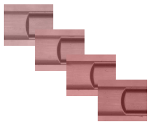
Figure 5. Capillary imbibition of silicone oils in glass tubes. (a) Representative invasion curves of silicone oils of different dynamic viscosity: 5.2 mPa s ( $\circ$), 19 mPa s ( $\diamond$), 46 mPa s ( $\triangle$) and 437 mPa s ( $\triangledown$). The two blank regions in each curve are the portions of the capillary hidden by the walls of the reservoirs. (b) Viscous deformation of the interface for 20 cSt oil. The apparent contact angle, $\theta$, decreases as the liquid slows down. The scale bars are 1 mm. The experimental parameter values are $L=100\,{\rm mm}$, $r=0.47\,{\rm mm}$, $\gamma =21\,{\rm mN}{\rm m}^{-1}$ and $\theta _{a}=0^\circ$.
To compare the experimental observations with the prediction of Washburn's law, we normalize the data using the length of the tube,  $L$, and the reference Washburn's imbibition time,
 \begin{equation} T\equiv \frac{4 \mu L^2}{2r\gamma \cos\theta_{a}+r^2\rho g h}, \end{equation}
which follows by imposing  $l(T)=L$ and $l_0=0$ in (2.8). As shown in figure 6(a), the rescaled data collapse onto a single master curve. However, this curve deviates systematically from Washburn's law (indicated by the solid line in the figure), which predicts an imbibition time roughly 20 % shorter than observed in the experiments. On a log–log scale, shown in figure 6(b), we observe a slow decrease of the growth exponent, with an average $\bar n\approx 0.55$ in the range of time span of the experimental data. Therefore, the discrepancy cannot be attributed to an offset due to edge effects.

Figure 6. Data collapse for the spontaneous imbibition of oils of different viscosity in (a) linear and (b) logarithmic scales. The length of the front is rescaled by the length of the tube,  $L$, and time is rescaled by the filling time, $T$, predicted by Washburn's law (solid line). The experimental uncertainty is calculated as half of the maximum resolution of the measurement, and is comparable to the symbol size in (a).
We now compare the experimental results with the theoretical model presented in § 4. First, let us analyse the characteristic magnitude of the different terms in the force balance, (2.10). In the experiments the Laplace number varies between  $La=2.5\times 10^{-2}$ and $La=1.6\times 10^{2}$, $Bo$ varies between $Bo=0.255$ and $Bo=0.326$, and we assume that $\epsilon =10^{-6}$ (de Gennes, Brochard-Wyart & Quéré Reference de Gennes, Brochard-Wyart and Quéré2013). Figure 2(c) shows the theoretical prediction of the magnitude of the different terms in the force balance for $La=10$, $Bo=0$, $\epsilon =10^{-6}$ and $\theta _{a}=0^\circ$ as a representative case of the experimental parameters (we found that the effect of both $La$ and $Bo$ in the experimental range is negligible). From the figure we expect that the acceleration of the liquid is negligible for $\hat t >10^0$, or, equivalently, $t/{T}>10^{-5}$. Moreover, during the linear-growth regime we expect that the hydrodynamic resistance of the meniscus is several times larger than the inertial resistance, which decays much faster for times $t/T>10^{-2}$ (i.e. in the range captured by our measurements). Since the silicone oils completely wet the capillary tube walls, i.e. $\theta _{a}=0^\circ$, we make the small-angle approximation $\cos \theta \approx 1 - \theta ^2/2$. Accordingly, (2.10) reduces to
 \begin{equation} 0 = 1 + Bo - 4 \hat l \hat u - \frac{1}{2}(9\ln \epsilon^{{-}1})^{2/3}\hat u^{2/3}. \end{equation}
For  $Bo=0$, (5.4) recovers the model proposed by Primkulov et al. (Reference Primkulov, Chui, Pahlavan, MacMinn and Juanes2020).
The dashed lines in figures 6(a) and 6(b) show the prediction of (5.4), which agrees very well with the experimental data. In particular, the theoretical prediction captures the slow variation of the growth exponent, which remains above the Washburn's limit for the whole of the imbibition process.
Let us now discuss the cross-over between the linear and the diffusive-like growth regimes presented in § 4 for the experimental conditions. From table 1, it follows that
 \begin{equation} l_{c} = \left(\frac{15}{32(1+Bo)}\right)^{1/2} \ln\epsilon^{{-}1} r, \end{equation}
and
 \begin{equation} \Delta\lambda = \tfrac{24}{5}. \end{equation}
In our experiments,  $\epsilon \approx 10^{-6}$ and $r=0.47\,{\rm mm}$, while the average Bond number is $Bo\approx 0.3$. Therefore, the cross-over is located at
 \begin{equation} l_{c} \approx 10\,{\rm mm}. \end{equation}
Note, however, that  $\exp (\pm 24/5)\approx 10^{\pm 2}$. Therefore, the range of the cross-over is
 \begin{equation} 10^{{-}1}\,{\rm mm} \leq l \leq 10^3\,{\rm mm}. \end{equation}
Because the length of the tube is  $L=100\,{\rm mm}$, the front never crosses over to Washburn's regime. Note that, to achieve a fully developed diffusive-like growth, one would need a tube with a very small aspect ratio, $r/L \approx 10^{-4}$.
5.3. Partially wetting fluids: imbibition of water
Let us now discuss our experimental results for the imbibition of water. As shown in figure 7(a), the experimental measurements of the invasion length as a function of time also collapse onto a single master curve when normalising time by Washburn's imbibition time  $T$. However, a plot on a log–log scale, presented in figure 7(b), shows that the local exponent varies significantly during the imbibition process, and it is not possible to identify a single apparent exponent that describes the dynamics. This rapid variation is not only due to the effect of the contact line, but also due to inertia. Unlike silicone oils, the relatively high capillary speed of water, $\gamma /\mu \approx 81\,{\rm m}\,{\rm s}^{-1}$, leads to a Laplace number $La\approx 2\times 10^4$, making the effect of inertial resistance non-negligible. On the other hand, the relatively high advancing contact angle of water on glass, $\theta _{a} = 69^\circ$, implies that the dynamic term in (2.12) is relatively small. Therefore, we expand $f(\hat u)$ in (2.10) up to linear order. This gives the equation of motion
 \begin{equation} 0 = \cos\theta_{a}+Bo- 4 \hat l \hat u - \frac{3}{2} La \hat u^2 - 3 \frac{\sin\theta_{a}}{\theta_{a}^2} \ln\epsilon^{{-}1} \hat u. \end{equation}
The dashed curves in figure 7(a,b) show the prediction of this equation, using  $Bo=0.096$ and $\epsilon =10^{-6}$, which captures the experimental data, including the slow variation of the apparent growth exponent.

Figure 7. Data collapse for water invading dry glass tubes in (a) linear and (b) logarithmic scales. Symbols correspond to different repetitions of the same experiment. The experimental uncertainty is calculated as half of the maximum resolution of the measurement, and is comparable to the symbol size in (a) and represented by the error bars in (b). The experimental parameter values are  $L=100\,{\rm mm}$, $r=0.47\,{\rm mm}$, $\gamma =72\,{\rm mN}\,{\rm m}^{-1}$, $\theta _{a} = 69^\circ$ and $\mu =0.89\,{\rm mPa}\,{\rm s}$.
Following the approach presented in § 4, we find the location of the cross-over and its range
 \begin{equation} l_{c} = \frac{\sin\theta_{a}}{4\theta_{a}^2}\left(1+2\sqrt{1+\phi}\right)r\ln\epsilon^{{-}1}, \end{equation}
and
 \begin{equation} \Delta \lambda = \frac{4+8\sqrt{1+\phi}}{3\sqrt{1+\phi}}, \end{equation}
where
 \begin{equation} \phi\equiv\frac{1}{2}(\cos\theta_{a}+Bo)\left(\frac{\theta_{a}^2}{\sin\theta_{a}\ln\epsilon^{{-}1}}\right)^2 La \end{equation}
quantifies the strength of inertial resistance relative to the hydrodynamic resistance of the meniscus. The limits of dominant inertia or dynamic angle of table 1 follow from (5.10) and (5.11) by taking the limits  $\phi \gg 1$ and $\phi \ll 1$, respectively. In our experiments, $\phi \approx 61$; hence, the cross-over is located at $l_{c} \approx 18\,{\rm mm}$ and covers the range $1\,{\rm mm}\leq l \leq 3\times 10^2\,{\rm mm},$ i.e. beyond the full imbibition of the capillary tube.
6. Conclusions
In this work we have shown that capillary imbibition is a long cross-over dynamics from a linear-growth regime to the diffusive-like growth of Washburn's law, and have provided a first-time systematic rationale of the deviation caused by the cross-over. The long cross-over is caused by the slow, power-law decay of the inertial and dynamic contact angle sources of resistance with the speed of the front. As a result, the front crosses over to Washburn's law over a range
 \begin{equation} l_{c} \exp (-\Delta \lambda) \leq l \leq l_{c} \exp (\Delta \lambda), \end{equation}
which is controlled by the cross-over location,
 \begin{equation} l_{c}\propto r, \end{equation}
and width,  $\Delta \lambda$. The cross-over location increases with the effect of inertia, controlled by the Laplace number, $La$, and dynamic angle, which is governed by the ratio of the size of the meniscus to the microscopic contact-line length scale, $\epsilon ^{-1}$. The width of the cross-over is determined by the power-law exponent, $\alpha$, of the corresponding resistance term, increasing from $\Delta \lambda =8/3$ for $\alpha =2$ (inertia) and $\Delta \lambda = 4$ for $\alpha =1$ (high dynamic contact angle), to $\Delta \lambda = 24/5$ for $\alpha =2/3$ (low dynamic contact angle). Because the cross-over range scales with the tube radius, we expect that it also dominates the dynamics at small scales. For instance, in the case of a completely wetting liquid invading a microchannel of radius $r=100\,\mathrm {\mu }{\rm m}$, we obtain $l_c\approx 1\,{\rm mm}$, and a cross-over that lasts up to $l\approx 10\,{\rm cm}$.
The experiments presented in this work illustrate the non-universality of the cross-over as the effects of inertia and dynamic angle compete in determining the front dynamics. Figure 8 shows the growth exponent,  $n$, calculated from (4.17) for the experimental systems studied in this paper: silicone oil, as an example of a completely wetting fluid with negligible inertial resistance, and water as an example of a partially wetting liquid with relatively high inertial resistance. For both liquids, the cross-over from the linear regime ( $n=1$) to Washburn's regime ( $n=1/2$) extends over the whole duration of the imbibition process. However, for water, the exponent is closer to Washburn's law when the front position is close to the end of the tube, while for silicone oil, the exponent is somehow larger, indicating a longer cross-over.

Figure 8. Exponent of the growth law  $l(t)\sim t^n$ as a function of the logarithm of the normalized penetration length into a capillary tube, $l/L$. The solid and dashed lines correspond to the theoretical predictions for silicone oils and water, respectively. The cross-over from the linear regime ( $n=1$) to the diffusive-like regime of Washburn's law ( $n=1/2$) extends over several decades of the front's position, and beyond the tube's length $L$. The shaded region corresponds to the range of observations in the experiments, with $L=100\,{\rm mm}$.
The slowly slowing-down dynamics studied in this paper is likely to influence capillary imbibition in other systems of interest, for instance, in the case of two fluid phases (Hultmark, Aristoff & Stone Reference Hultmark, Aristoff and Stone2011), complex geometries (Reyssat et al. Reference Reyssat, Courbin, Reyssat and Stone2008; Ouali et al. Reference Ouali, McHale, Javed, Trabi, Shirtcliffe and Newton2013; Gorce, Hewitt & Vella Reference Gorce, Hewitt and Vella2016) or through elastic media (Kim & Mahadevan Reference Kim and Mahadevan2006; Cambau, Bico & Reyssat Reference Cambau, Bico and Reyssat2011). Our results can also be of relevance in applications where control over the growth of a front is needed, for example, in front microfluidics (Trejo-Soto et al. Reference Trejo-Soto, Costa-Miracle, Rodríguez-Villarreal, Cid, Alarcón and Hernández-Machado2016).
Acknowledgements
We thank M. Pradas, G. McHale and E. Corvera Poiré for useful discussions; B. Orme and J. Rawlings for kindly providing viscosity measurements for our samples; and P. Agrawal for sharing his expertise in image analysis. We acknowledge industrial advice from V. Williams (Cellix Ltd), and D. Hislop (Sustainable Engine Systems Ltd).
Funding
E.R.-G. and R.L.-A. acknowledge support from EPSRC (grant no. EP/P024408/1). G.G.W. acknowledges support from EPSRC (grant no. EP/P026613/1). A.H.-M. acknowledges support from Ministerio de Ciencia e Innovación (Spain) under project PID2019-106063GB-100. I.P. acknowledges support from Ministerio de Ciencia, Innovación y Universidades MCIU/AEI/FEDER for financial support under grant agreement PGC2018-098373-B-100 AEI/FEDER-EU, from Generalitat de Catalunya under project 2017SGR-884, Swiss National Science Foundation Project No. 200021-175719. A.H.-M. and I.P. acknowledge the EU Horizon 2020 program through 766972-FET-OPEN NANOPHLOW.
Declaration of interests
The authors report no conflict of interest.
Author contributions
R.L.-A., A.H.-M. and I.P. devised the research. R.L.-A., E.R.-G., A.H.-M., and I.P. developed the theoretical model. G.G.W. and R.L.-A. designed the experiments. S.A., S.L. and C.M. carried out the experiments. G.G.W. and R.L.-A. analysed the data. R.L.-A. wrote the manuscript with input from all authors.


 Open access