1. Introduction
Idealized flow conditions often provide attractive features relative to furthering turbulent wall-flow theory, clarifying Reynolds number scaling and discerning the dynamics. Unfortunately, attaining and accurately quantifying such idealized flow conditions in a laboratory experiment often proves to be a highly non-trivial, if not unattainable, objective. Given this, the results documented in the study by Ferro, Fallenius & Fransson (Reference Ferro, Fallenius and Fransson2021), relative to the turbulent asymptotic suction boundary layer (TASBL), constitutes an unusual and significant contribution.
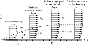
A defining property of the asymptotic suction boundary layer (laminar or turbulent) is a mass flux condition through the bounding surface that causes the boundary layer thickness  $\delta$ (or other outer length scale, e.g. displacement or momentum thickness) to remain fixed with downstream distance, $x$. Thus, in the asymptotic flow for a given $\delta$ and free stream velocity, $U_{\infty }$, there is a wallward transpiration velocity, $V_0$, whose effect identically counteracts the tendency for the boundary layer to otherwise grow with increasing $x$. As might be anticipated, the balance needed to attain this asymptotic state is uniquely defined for each $U_{\infty }$ and $\delta$. In the laminar ASBL, the precise condition of fully developed flow (zero streamwise gradient) allows one to directly solve for the asymptotic velocity profile in terms of the suction velocity. In the turbulent case, precise parameter settings are also needed, with too much mass removal leading to downstream relaminarization and too little being insufficient to abate boundary layer growth. Ferro et al. (Reference Ferro, Fallenius and Fransson2021) provide compelling evidence that their experiments attain the delicate balance required to create the TASBL state within a relatively short streamwise fetch and over a significant range of Reynolds numbers.
The momentum equation for the laminar ASBL and the mean momentum equation for the TASBL have simplifying analytical features that make them attractive for theoretical studies of transition, edge states and exact coherent structures (Kreilos et al. Reference Kreilos, Veble, Schneider and Eckhardt2013; Khapko et al. Reference Khapko, Duguet, Kreilos, Schlatter, Eckhardt and Henningson2014; Zammert, Fischer & Eckhardt Reference Zammert, Fischer and Eckhardt2016). In particular, these are $x$-invariant wall flows (statistically homogeneous in the TASBL case) that also have a constant velocity and irrotational free stream. Relative to the TASBL, Ferro et al. (Reference Ferro, Fallenius and Fransson2021) identify a number of open questions that their experiments then convincingly address. Perhaps the most fundamental of these is whether the TASBL state can be attained in a reasonable laboratory experiment – an aim that, based upon their large eddy simulation results, Bobke, Orlu & Schlatter (Reference Bobke, Orlu and Schlatter2016) asserted was practically impossible. Similarly, Ferro et al. (Reference Ferro, Fallenius and Fransson2021) describe that, owing to the paucity of data, the functional form and scaling behaviours associated with the mean velocity profile are not convincingly known – although a number of plausible proposals have been made regarding a logarithmic and/or bi-logarithmic region in addition to the profile in the viscous sublayer (e.g. Black & Sarnecki Reference Black and Sarnecki1958; Tennekes Reference Tennekes1964; Vigdorovich Reference Vigdorovich2016). Regarding the properties of the turbulence in the TASBL, even less is known than is for the mean velocity, and here, Ferro et al. (Reference Ferro, Fallenius and Fransson2021) present the clearest documentation to date of the streamwise, $u$, velocity fluctuation variance profiles and their underlying spectral properties.
2. Overview
The TASBL experiments of Ferro et al. (Reference Ferro, Fallenius and Fransson2021) were conducted in the Minimum Turbulence Level (MTL) wind tunnel at KTH. The use of the MTL wind tunnel is significant relative to the fidelity of the experiments, as this wind tunnel is one of the world's premier wall-flow stability and turbulence facilities. Owing to the size of the MTL wind tunnel, the experiments had a physical scale that is approximately $2.5$ times larger than any previous study of the TASBL. This feature connects to the attainable Reynolds number range and the spatial resolution of the turbulence measurements.
Achieving the desired flow conditions required a number of non-trivial modifications to the baseline MTL facility test section configuration, and here is where one gains an appreciation for the careful design and meticulous attention to detail that Ferro et al. (Reference Ferro, Fallenius and Fransson2021) employ. As described in considerable detail in § 2 of the manuscript, the requisite wall suction was made possible through the use of a series of eight perforated titanium plates that spanned the entire test section width and extended approximately 6.5 m in the flow direction (see manuscript figures 2 and 3). Each plate was connected to a series of manifolds and an individual control valve that allowed a homogeneous suction to be applied and continuously adjusted. Figure 8 of the manuscript documents an impressive test of the precision and control of the suction system and the overall quality of the flow produced. Here, the data are shown to exhibit excellent agreement with the laminar ASBL analytical solution over the entire profile.
Establishing the TASBL flow involved a number of additional considerations, some of which required adapting the MTL wind tunnel configuration to allow for measurements that accurately quantify the TASBL flow. The relevant actions included verifying that a canonical (zero pressure gradient) flow develops over the perforated plate system under zero transpiration, designing and implementing a boundary layer extraction system near the start of the perforated panel array to set the inflow conditions and installing a probe traversing system that accommodates precise sensor positioning relative to the perforated wall. Table 1 in the manuscript documents that the parameters and flow conditions for the canonical flow are precisely established over a friction Reynolds number range of $2500 \lesssim R_{\tau } \lesssim 6700$, while tables 2 and 3 respectively show the parameters for which TASBL conditions were obtained at $x = 4.80\ \textrm {m}$ and $x = 6.06\ \textrm {m}$.
Here, it is worth emphasizing that attaining the TASBL states documented in tables 2 and 3 involved the painstaking process of wall suction and flow speed adjustment described in § 3.2 of the manuscript. This procedure produced the zero boundary layer growth conditions evidenced in figure 10. These results are distinctive as they are the first to convincingly show that the delicate balance of the TASBL can be attained in the laboratory over a range of Reynolds number, boundary layer thickness and flow speed conditions. In this regard, Ferro et al. (Reference Ferro, Fallenius and Fransson2021) show that, for any particular $\delta$, the parameter $\varGamma = -V_0/U_{\infty }$ is the only one requiring adjustment to attain the necessary zero growth condition, and here they reveal that $\varGamma$ is a mildly decreasing function of Reynolds number.
Upon producing a range of TASBL states, the authors subsequently investigate the properties of the mean velocity profile and $u$ fluctuations. Regarding the mean velocity profile, their results evidence that the TASBL $U(y)$ profile has a clear and extensive region of logarithmic dependence, and that the profile has essentially no outer wake region. Distinct from the canonical wall flows, the logarithmic layer in the TASBL most convincingly attains universality when represented under outer normalization for both the wall-normal distance (i.e. $y/\delta$) and the velocity (i.e. $U/U_{\infty }$). This behaviour is exemplified in figure 1 herein (reproduced from figure 16 in the manuscript), which shows the outer-normalized indicator function $\varXi = y \textrm {d}(U/U_{\infty })/{\textrm {d}y}$ over the full range of TASBLs listed in the manuscript's table 2. As is apparent, the profiles of figure 1(b) convincingly merge over a large outer region, and the domain of constant $\varXi$ (indicating logarithmic dependence) extends over approximately $40\,\%$ of the flow domain. As a percentage, this is a much more extensive logarithmic layer than seen in the canonical turbulent wall flows.
The $u$ variance profiles of figure 20 are of considerably reduced magnitude relative to the flat plate boundary layer flow. These measurements also reveal that the inner-normalized peak position of these profiles is fixed across the measurement range of TASBL conditions and at the same location ($y^+ \simeq 15$) as in the canonical flow. Dramatic changes occur in the outer region turbulence structure under the influence of wall suction. This is evident in the virtual annihilation of the outer plateau region that is a characteristic feature of the canonical boundary layer. Consistently, spectrograms of the $u$ fluctuations indicate that wall suction almost completely removes the signature of the large-scale outer region motions. In their documentation of the $u$ fluctuation properties, Ferro et al. (Reference Ferro, Fallenius and Fransson2021) provide a careful analysis of spatial resolution effects. This analysis is important as it allows one to reliably discern between Reynolds number dependence and signal attenuation owing to finite probe-scale spatial averaging effects.
3. Broader implications
Like a small number of other non-canonical flows, the laminar ASBL has an exact analytical solution and upon transition to turbulence the associated TASBL has a distinct simplifying characteristic (i.e. zero boundary layer growth). Broader consideration here brings to mind the notion of a canonical non-canonical wall flow. Such flows are part of a family of those that are more complex than the canonical wall flows, but that contain attractive analytical and simplifying characteristics whose study provides a context for better understanding turbulent wall flows more broadly. Candidate flows in this regard include the favourable pressure gradient sink turbulent boundary layer flow, turbulent Taylor Couette flow, turbulent Couette–Poiseuille flow and, in the three-dimensional case, the von Kármán rotating disk boundary layer, as well as the present TASBL flow.
Consistent with the above assertion, the study by Ferro et al. (Reference Ferro, Fallenius and Fransson2021) provides new insights into wall-flow structure. Namely, it reveals that the TASBL mean velocity profile contains a region of logarithmic dependence that comprises a vastly larger fraction of the flow domain than seen in the canonical wall flows. While more study of the TASBL is required to better understand why this occurs, one can readily surmise that the underlying conditions necessary to yield a logarithmic profile are clearly not necessarily constrained to a narrow physical space inertial sublayer, i.e. as the study of the canonical flows leads one to conclude.


1. Introduction
Idealized flow conditions often provide attractive features relative to furthering turbulent wall-flow theory, clarifying Reynolds number scaling and discerning the dynamics. Unfortunately, attaining and accurately quantifying such idealized flow conditions in a laboratory experiment often proves to be a highly non-trivial, if not unattainable, objective. Given this, the results documented in the study by Ferro, Fallenius & Fransson (Reference Ferro, Fallenius and Fransson2021), relative to the turbulent asymptotic suction boundary layer (TASBL), constitutes an unusual and significant contribution.
A defining property of the asymptotic suction boundary layer (laminar or turbulent) is a mass flux condition through the bounding surface that causes the boundary layer thickness $\delta$ (or other outer length scale, e.g. displacement or momentum thickness) to remain fixed with downstream distance, $x$. Thus, in the asymptotic flow for a given $\delta$ and free stream velocity, $U_{\infty }$, there is a wallward transpiration velocity, $V_0$, whose effect identically counteracts the tendency for the boundary layer to otherwise grow with increasing $x$. As might be anticipated, the balance needed to attain this asymptotic state is uniquely defined for each $U_{\infty }$ and $\delta$. In the laminar ASBL, the precise condition of fully developed flow (zero streamwise gradient) allows one to directly solve for the asymptotic velocity profile in terms of the suction velocity. In the turbulent case, precise parameter settings are also needed, with too much mass removal leading to downstream relaminarization and too little being insufficient to abate boundary layer growth. Ferro et al. (Reference Ferro, Fallenius and Fransson2021) provide compelling evidence that their experiments attain the delicate balance required to create the TASBL state within a relatively short streamwise fetch and over a significant range of Reynolds numbers.
The momentum equation for the laminar ASBL and the mean momentum equation for the TASBL have simplifying analytical features that make them attractive for theoretical studies of transition, edge states and exact coherent structures (Kreilos et al. Reference Kreilos, Veble, Schneider and Eckhardt2013; Khapko et al. Reference Khapko, Duguet, Kreilos, Schlatter, Eckhardt and Henningson2014; Zammert, Fischer & Eckhardt Reference Zammert, Fischer and Eckhardt2016). In particular, these are $x$-invariant wall flows (statistically homogeneous in the TASBL case) that also have a constant velocity and irrotational free stream. Relative to the TASBL, Ferro et al. (Reference Ferro, Fallenius and Fransson2021) identify a number of open questions that their experiments then convincingly address. Perhaps the most fundamental of these is whether the TASBL state can be attained in a reasonable laboratory experiment – an aim that, based upon their large eddy simulation results, Bobke, Orlu & Schlatter (Reference Bobke, Orlu and Schlatter2016) asserted was practically impossible. Similarly, Ferro et al. (Reference Ferro, Fallenius and Fransson2021) describe that, owing to the paucity of data, the functional form and scaling behaviours associated with the mean velocity profile are not convincingly known – although a number of plausible proposals have been made regarding a logarithmic and/or bi-logarithmic region in addition to the profile in the viscous sublayer (e.g. Black & Sarnecki Reference Black and Sarnecki1958; Tennekes Reference Tennekes1964; Vigdorovich Reference Vigdorovich2016). Regarding the properties of the turbulence in the TASBL, even less is known than is for the mean velocity, and here, Ferro et al. (Reference Ferro, Fallenius and Fransson2021) present the clearest documentation to date of the streamwise, $u$, velocity fluctuation variance profiles and their underlying spectral properties.
2. Overview
The TASBL experiments of Ferro et al. (Reference Ferro, Fallenius and Fransson2021) were conducted in the Minimum Turbulence Level (MTL) wind tunnel at KTH. The use of the MTL wind tunnel is significant relative to the fidelity of the experiments, as this wind tunnel is one of the world's premier wall-flow stability and turbulence facilities. Owing to the size of the MTL wind tunnel, the experiments had a physical scale that is approximately $2.5$ times larger than any previous study of the TASBL. This feature connects to the attainable Reynolds number range and the spatial resolution of the turbulence measurements.
Achieving the desired flow conditions required a number of non-trivial modifications to the baseline MTL facility test section configuration, and here is where one gains an appreciation for the careful design and meticulous attention to detail that Ferro et al. (Reference Ferro, Fallenius and Fransson2021) employ. As described in considerable detail in § 2 of the manuscript, the requisite wall suction was made possible through the use of a series of eight perforated titanium plates that spanned the entire test section width and extended approximately 6.5 m in the flow direction (see manuscript figures 2 and 3). Each plate was connected to a series of manifolds and an individual control valve that allowed a homogeneous suction to be applied and continuously adjusted. Figure 8 of the manuscript documents an impressive test of the precision and control of the suction system and the overall quality of the flow produced. Here, the data are shown to exhibit excellent agreement with the laminar ASBL analytical solution over the entire profile.
Establishing the TASBL flow involved a number of additional considerations, some of which required adapting the MTL wind tunnel configuration to allow for measurements that accurately quantify the TASBL flow. The relevant actions included verifying that a canonical (zero pressure gradient) flow develops over the perforated plate system under zero transpiration, designing and implementing a boundary layer extraction system near the start of the perforated panel array to set the inflow conditions and installing a probe traversing system that accommodates precise sensor positioning relative to the perforated wall. Table 1 in the manuscript documents that the parameters and flow conditions for the canonical flow are precisely established over a friction Reynolds number range of $2500 \lesssim R_{\tau } \lesssim 6700$, while tables 2 and 3 respectively show the parameters for which TASBL conditions were obtained at $x = 4.80\ \textrm {m}$ and $x = 6.06\ \textrm {m}$.
Here, it is worth emphasizing that attaining the TASBL states documented in tables 2 and 3 involved the painstaking process of wall suction and flow speed adjustment described in § 3.2 of the manuscript. This procedure produced the zero boundary layer growth conditions evidenced in figure 10. These results are distinctive as they are the first to convincingly show that the delicate balance of the TASBL can be attained in the laboratory over a range of Reynolds number, boundary layer thickness and flow speed conditions. In this regard, Ferro et al. (Reference Ferro, Fallenius and Fransson2021) show that, for any particular $\delta$, the parameter $\varGamma = -V_0/U_{\infty }$ is the only one requiring adjustment to attain the necessary zero growth condition, and here they reveal that $\varGamma$ is a mildly decreasing function of Reynolds number.
Upon producing a range of TASBL states, the authors subsequently investigate the properties of the mean velocity profile and $u$ fluctuations. Regarding the mean velocity profile, their results evidence that the TASBL $U(y)$ profile has a clear and extensive region of logarithmic dependence, and that the profile has essentially no outer wake region. Distinct from the canonical wall flows, the logarithmic layer in the TASBL most convincingly attains universality when represented under outer normalization for both the wall-normal distance (i.e. $y/\delta$) and the velocity (i.e. $U/U_{\infty }$). This behaviour is exemplified in figure 1 herein (reproduced from figure 16 in the manuscript), which shows the outer-normalized indicator function $\varXi = y \textrm {d}(U/U_{\infty })/{\textrm {d}y}$ over the full range of TASBLs listed in the manuscript's table 2. As is apparent, the profiles of figure 1(b) convincingly merge over a large outer region, and the domain of constant $\varXi$ (indicating logarithmic dependence) extends over approximately $40\,\%$ of the flow domain. As a percentage, this is a much more extensive logarithmic layer than seen in the canonical turbulent wall flows.
Figure 1. Indicator function, $\varXi$ for the TASBL vs the inner-scaled (a) and outer-scaled (b) wall-normal coordinate. Adapted from figure 16 of Ferro et al. (Reference Ferro, Fallenius and Fransson2021).
The $u$ variance profiles of figure 20 are of considerably reduced magnitude relative to the flat plate boundary layer flow. These measurements also reveal that the inner-normalized peak position of these profiles is fixed across the measurement range of TASBL conditions and at the same location ( $y^+ \simeq 15$) as in the canonical flow. Dramatic changes occur in the outer region turbulence structure under the influence of wall suction. This is evident in the virtual annihilation of the outer plateau region that is a characteristic feature of the canonical boundary layer. Consistently, spectrograms of the $u$ fluctuations indicate that wall suction almost completely removes the signature of the large-scale outer region motions. In their documentation of the $u$ fluctuation properties, Ferro et al. (Reference Ferro, Fallenius and Fransson2021) provide a careful analysis of spatial resolution effects. This analysis is important as it allows one to reliably discern between Reynolds number dependence and signal attenuation owing to finite probe-scale spatial averaging effects.
3. Broader implications
Like a small number of other non-canonical flows, the laminar ASBL has an exact analytical solution and upon transition to turbulence the associated TASBL has a distinct simplifying characteristic (i.e. zero boundary layer growth). Broader consideration here brings to mind the notion of a canonical non-canonical wall flow. Such flows are part of a family of those that are more complex than the canonical wall flows, but that contain attractive analytical and simplifying characteristics whose study provides a context for better understanding turbulent wall flows more broadly. Candidate flows in this regard include the favourable pressure gradient sink turbulent boundary layer flow, turbulent Taylor Couette flow, turbulent Couette–Poiseuille flow and, in the three-dimensional case, the von Kármán rotating disk boundary layer, as well as the present TASBL flow.
Consistent with the above assertion, the study by Ferro et al. (Reference Ferro, Fallenius and Fransson2021) provides new insights into wall-flow structure. Namely, it reveals that the TASBL mean velocity profile contains a region of logarithmic dependence that comprises a vastly larger fraction of the flow domain than seen in the canonical wall flows. While more study of the TASBL is required to better understand why this occurs, one can readily surmise that the underlying conditions necessary to yield a logarithmic profile are clearly not necessarily constrained to a narrow physical space inertial sublayer, i.e. as the study of the canonical flows leads one to conclude.
Declaration of interests
The author reports no conflict of interest.