3.1. The turbulent statistics for vorticity and acoustic modes

For velocity fields dominated by the vorticity mode, figure 2 presents the first- and second-moment statistics of the streamwise velocity. As shown in figure 2(a), the profiles of mean velocity $\bar {u}^+$ for all cases reasonably agree with the wall law in the range of $y^+<5$, but only the distribution for case M0 exhibits a good agreement with the log law where compressibility is negligibly weak. With increasing $M$, the profiles gradually deviate from the log law. After considering variations in mean density in figure 2(b), it is observed that the profiles of Van Driest transformed (Van Driest Reference Van Driest1951) mean velocity $\bar {u}_{vd}$ for all cases agree well with each other in both near-wall and log-law regions. Similarly, for velocity fluctuations intensities $u^{\prime +}_{rms}$ in figure 2(c), only the profile of case M0 collapses with the incompressible profile (Jiménez et al. Reference Jiménez, Hoyas, Simens and Mizuno2010), while the profiles of other cases with higher $M$ gradually deviate from the incompressible profile. Following the relations of strong Reynolds analogy (Morkovin Reference Morkovin1962), when the variation of mean density is taken into account, it can be seen in figure 2(d) that the profiles of density-scaled fluctuation intensities exhibit superior clustering and collapse compared with those of $u^{\prime +}_{rms}$. The obtained results not only validate the accuracy of the present data but also demonstrate the efficacy of utilizing Morkovin's hypothesis to map the statistics of compressible velocity fields onto their incompressible counterparts.

Figure 2. Statistical properties of streamwise velocity: (a) mean velocity $\bar {u}^+$; (b) Van Driest transformed mean velocity $\bar{u}_{vd}^+$; (c) fluctuation intensity; (d) density scaled fluctuation intensity. The dot–dashed and dashed lines denote the wall law $u^+=y^+$ and the log law $u^+=\log {(y^+)}/0.41+5.2$, respectively. The circles indicate the reference data of an incompressible TBL with ${{Re}}_\tau =580$ from Jiménez et al. (Reference Jiménez, Hoyas, Simens and Mizuno2010). The diamonds denote a $M=8$ TBL with ${{Re}}_\tau =398$ from Duan et al. (Reference Duan, Beekman and Martín2011).

Considering that pressure fluctuations in compressible TBLs are mainly influenced by both the vorticity mode and acoustic mode (Phillips Reference Phillips1960; Lilley Reference Lilley1963), figure 3 presents the profiles of vorticity fluctuation intensities $\omega _{rms}^{\prime +}$ and dilatation fluctuation intensities $\theta _{rms}^{\prime +}$, which can characterize the vorticity mode and acoustic mode to a certain extent, respectively. As shown in figure 3(a), the profiles of $\omega _{rms}^{\prime +}$ for all cases collapse well with each other at the fixed ${{Re}}_\tau$, indicating that the profiles of $\omega _{rms}^{\prime +}$ are almost not affected by increasing $M$. The magnitude of the vorticity mode seems to be controlled only by the parameter of ${{Re}}_\tau$. For dilatation fluctuations, the increase in $M$ monotonically enhances $\theta _{rms}^{\prime +}$ especially near the wall, as shown in figure 3(b). The magnitude of $\theta _{rms}^{\prime +}$ gradually weakens as the wall-normal position moves away from the wall. The distribution trends of $\omega _{rms}^{\prime +}$ and $\theta _{rms}^{\prime +}$ are consistent with the DNS data reported by Bernardini & Pirozzoli (Reference Bernardini and Pirozzoli2011). These findings imply the presence of intrinsic scaling relations, particularly when the vorticity and acoustic modes are properly isolated. Specifically, the contribution of the vorticity mode to pressure fluctuations is independent of $M$, while the contribution of the acoustic mode exhibits a monotonic increase with $M$.

Figure 3. (a) Vorticity fluctuation intensities $\omega _{rms}^{\prime +}$ and (b) dilatation fluctuation intensities $\theta _{rms}^{\prime +}$.

3.2. The direct scaling relations of pressure fluctuations

To illustrate the scaling relations between pressure fluctuations and $M$ directly, figure 4 shows the profiles of pressure fluctuation intensities $p_{rms}^{\prime +}$ in both the outer and inner scales, respectively. The profiles of all cases exhibit a similar trend that $p_{rms}^{\prime +}$ increases from its value at the wall and reaches the global maximum at $y^+\approx 12$ and then gradually decays to a plateau value out of the boundary layer where acoustic radiations dominate. As indicated by the black arrow in figure 4(a), the increase in $M$ overall enhances $p_{rms}^{\prime +}$ monotonically, corresponding to stronger acoustic modes in cases of higher $M$. The profile of the M0 case closely aligns with the reference data of an incompressible TBL (Jiménez et al. Reference Jiménez, Hoyas, Simens and Mizuno2010). Within the boundary layer, the near-wall enhancement clearly shown in figure 4(b) is a consequence of the stronger genuine compressibility in higher-$M$ cases, as demonstrated by $\theta _{rms}^{\prime +}$ in figure 3(b). In the far field, the enhancement in supersonic and hypersonic cases should be attributed to the Mach-wave radiation, which is induced by the supersonic convection eddies within TBLs. Because of the comprehensive contributions from the vorticity and acoustic modes, considering the variations in mean quantities may not be a viable solution when mapping the compressible profile of pressure fluctuations to the incompressible counterpart. Instead, removing the contribution of acoustic modes to pressure fluctuations is expected to work.

Figure 4. Intensities of pressure fluctuations $p_{rms}^{\prime +}$ shown in (a) the outer scale and (b) the inner scale. The circles indicate the reference data of an incompressible TBL with ${{Re}}_\tau =690$ from Jiménez et al. (Reference Jiménez, Hoyas, Simens and Mizuno2010). The squares and diamonds denote $M=2$ and 4 TBLs with ${{Re}}_\tau =508$ and 506, respectively, from Bernardini & Pirozzoli (Reference Bernardini and Pirozzoli2011).

For evaluating the scaling relations of wall and far-field pressure fluctuations, the variations of pressure fluctuation intensities versus $M$ are shown in figure 5. For wall pressure fluctuation intensities normalized by the free stream dynamic pressure $p_{rms}^{\prime }/q_\infty$, the data from measurements (grey square), simulations (red symbols) and prediction models (dashed lines) are collected in figure 5(a). Due to the limitations of pressure sensors in experiments, from light to dark colours, the grey squares indicate the uncorrected raw data, the corrected data by Corcos corrections (Corcos Reference Corcos1963) and the extended data further corrected based on an estimation of high-frequency spectra. It is shown that the corrected experimental data agree much better with simulation data than the original data. For compressible flows, Laganelli, Martellucci & Shaw (Reference Laganelli, Martellucci and Shaw1983) proposed an empirical model by extending an incompressible theory to compressible states, written as

(3.1)\begin{equation} p_{rms,w}^{\prime}/q_{\infty}=\frac{\sigma}{\left[0.5+\left(T_{w} / T_{r}\right)\left(0.5+0.09 M^{2}\right)+0.04 M^{2}\right]^{\phi}}, \end{equation}

where the two parameters $\sigma$ and $\phi$ are determined by fitting experimental data. Their original values are $\sigma =0.006$ and $\phi =0.64$. Considering the potential bias in historical experimental data, the predictions of the original Laganelli model exhibit an overall underestimation compared with the numerical data. Therefore, Ritos et al. (Reference Ritos, Drikakis and Kokkinakis2019a) improved the model by introducing a modified $\sigma =0.008$ based on fitting their iLES data in a range of $2.25\le M\le 8$, but significant deviations still occur at the relatively lower Mach number range of $M<2$. By optimizing both two parameters, the modified model with $\sigma =0.01$ and $\phi =0.75$ proposed by Zhang et al. (Reference Zhang, Wan, Liu, Sun and Lu2022) shows good performances in a wide Mach number range of $0\le M\le 8$. Pressure fluctuation intensities normalized by the wall unit ($p_{rms,\infty }^{\prime +}$) in the far-field are also presented in figure 5(b), where grey diamonds indicate experimental data, red and blue symbols indicate numerical data with quasiadiabatic and cooled walls, respectively. The distributions of $p_{rms,\infty }^{\prime +}$ show approximately monotonic linear growths with increasing $M$. Consequently, a simple linear relation expressed as $p_{rms,\infty }^{\prime +}=0.12M+0.08$, can be obtained by fitting these data.

Figure 5. Pressure fluctuation intensities with scaling models (a) at the wall and (b) in the far-field.

3.3. The intrinsic scaling relations of decomposed pressure components

In an effort to discern the respective contributions of vorticity and acoustic modes from the perspective of the generation mechanism of pressure fluctuations, we employ a decomposition method based on the governing equation of pressure fluctuations. This approach enables us to investigate the intrinsic scaling relations. Starting from the governing equations for mass and momentum in a Cartesian coordinate system written as

(3.2)\begin{gather} \frac{\partial \rho}{\partial t}+\frac{\partial \rho u_{j}}{\partial x_{j}}=0, \end{gather}

(3.3)\begin{gather} \frac{\partial \rho u_{i}}{\partial t}+\frac{\partial \rho u_{i} u_{j}}{\partial x_{j}}=-\frac{\partial p}{\partial x_{i}}+\frac{\partial \tau_{i j}}{\partial x_{j}}, \end{gather}

where $\tau _{i j}$ is the viscous stress tensor, take the divergence of the momentum equations (3.3) yielding

(3.4)\begin{equation} \frac{\partial^{2} p}{\partial x_{i} \partial x_{i}}=-\frac{\partial^{2}}{\partial x_{i} \partial x_{j}}\left(\rho u_{i} u_{j}-\tau_{i j}\right)-\frac{\partial}{\partial x_{i}} \frac{\partial \rho u_{i}}{\partial t} . \end{equation}

By subtracting the average of (3.4) from itself and combining the continuity equation (equation (3.2)), the governing equation of pressure fluctuations can be written as (Gerolymos, Sénéchal & Vallet Reference Gerolymos, Sénéchal and Vallet2007)

(3.5)\begin{align} \frac{\partial^{2} p^{\prime}}{\partial x_{i} \partial x_{i}}=\frac{\partial^{2}}{\partial x_{i} \partial x_{j}} \tau_{i j}^{\prime}-\frac{\partial^{2}}{\partial x_{i} \partial x_{j}}\left(2 \rho \tilde{u}_{i} u_{j}^{\prime \prime}+\rho^{\prime} \tilde{u}_{i} \tilde{u}_{j}\right)-\frac{\partial^{2}}{\partial x_{i} \partial x_{j}}\left(\rho u_{i}^{\prime \prime} u_{j}^{\prime \prime}-\overline{\rho u_{i}^{\prime \prime} u_{j}^{\prime \prime}}\right)+\frac{\partial^{2} \rho^{\prime}}{\partial t^{2}}. \end{align}

According to characteristics of the source terms on the right-hand side of (3.5), the pressure fluctuation can be decomposed into several components (Yu et al. Reference Yu, Xu and Pirozzoli2020; Zhang et al. Reference Zhang, Wan, Liu, Sun and Lu2022), $p^\prime =p_r+p_s+p_\tau +p_c+p_h$. These components individually satisfy

(3.6a)$$\begin{gather} \frac{\partial^{2} p_{r}}{\partial x_{i} \partial x_{i}}=-2 \frac{\partial \tilde{u}_{i}}{\partial x_{j}} \frac{\partial \rho u_{j}^{\prime \prime}}{\partial x_{i}}, \end{gather}$$

(3.6b)$$\begin{gather}\frac{\partial^{2} p_{s}}{\partial x_{i} \partial x_{i}}=-\frac{\partial^{2}}{\partial x_{i} \partial x_{j}}\left(\rho u_{i}^{\prime \prime} u_{j}^{\prime \prime}-\overline{\rho u_{i}^{\prime \prime} u_{j}^{\prime \prime}}\right), \end{gather}$$

(3.6c)$$\begin{gather}\frac{\partial^{2} p_{\tau}}{\partial x_{i} \partial x_{i}}=\frac{\partial^{2} \tau_{i j}^{\prime}}{\partial x_{i} \partial x_{j}}, \end{gather}$$

(3.6d)$$\begin{gather}\frac{\partial^{2} p_{c}}{\partial x_{i} \partial x_{i}}=\frac{\partial^{2} \rho^{\prime}}{\partial t^{2}}-\frac{\partial^{2}}{\partial x_{i} \partial x_{j}}\left(2 \rho \tilde{u}_{i} u_{j}^{\prime \prime}+\rho^{\prime} \tilde{u}_{i} \tilde{u}_{j}\right)+2 \frac{\partial \tilde{u}_{i}}{\partial x_{j}} \frac{\partial \rho u_{j}^{\prime \prime}}{\partial x_{i}}, \end{gather}$$

(3.6e)$$\begin{gather}\frac{\partial^{2} p_{h}}{\partial x_{i} \partial x_{i}}=0, \end{gather}$$

where the first two components $p_r$ and $p_s$ are so-called rapid and slow pressures similar to those in incompressible flow, caused by linear mean flow–turbulence interactions and nonlinear turbulence–turbulence interactions, respectively; the viscous pressure $p_\tau$ corresponds to the contribution of the viscous stress; the compressible pressure $p_c$ accounts for contributions of compressibility which is the principal representation of the essential nature of compressibility effects on the pressure statistics (Sarkar Reference Sarkar1992; Foysi et al. Reference Foysi, Sarkar and Friedrich2004; Tang et al. Reference Tang, Zhao, Wan and Liu2020); and the harmonic pressure $p_h$ is introduced to denote the contribution of streamwise boundary conditions (Pope Reference Pope2000). All the right-hand side source terms are obtained by discretization based on the DNS data. The Poisson equations of pressure components are solved by the Fourier–Galerkin scheme in a subdomain of the computational domain as shown in figure 6 with the specific boundary conditions given in table 3. The grid of the subdomain is the same as that of the DNS computation but truncated in the streamwise and wall-normal directions. In the streamwise direction, the subdomain spans over 800 points for all cases except case M8, which increases to 1200 points due to its smaller grid spacing. The location for analysis is at the streamwise midpoint of the subdomain. In the wall-normal direction, the subdomain spans over 280 points starting from the wall, and the wall-normal location of the upper boundary exceeds $3\delta$ ensuring acoustic radiation dominants here. Note that due to the evanescent nature of vortex waves and entropy waves out of boundary layers, other pressure components except $p_c$ are set to 0 at the far-field boundary, while the propagation nature of acoustic waves is mainly reflected in the compressible pressure $p_c$, so that $p_c=p^\prime$ is imposed at the far-field.

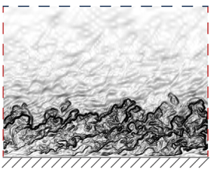
Figure 6. Schematic for the pressure decomposition. The subdomain of the numerical schlieren of the M8 case is drawn.

Table 3. Boundary conditions of the pressure fluctuation equations for each pressure component.

According to generation mechanisms of pressure fluctuations from the characteristics of the source terms, the compressible pressure $p_c$ is used to represent the contributions from the acoustic mode. Meanwhile, the sum of the remaining components, $p_i=p_r+p_s+p_\tau +p_h$, is nominally defined as the hydrodynamic pressure (quasi-incompressible component) denoting the contributions from the vorticity mode, resulting in $p^\prime =p_i+p_c$. The instantaneous fields of the original pressure fluctuations $p^{\prime +}$ as well as the compressible pressure $p_c^+$ and hydrodynamic pressure $p_i^+$ in wall scaling are depicted in figure 7, taking the M0, M2 and M8 cases as examples for brevity. For $p^{\prime +}$ fields in figure 7(a,b), pressure fluctuations are mainly associated with vortex structures within the boundary layer. In the far field, pressure fluctuations radiate as acoustic waves, which are relatively weak in case M0. As the Mach number increases, the amplitudes of radiating pressure fluctuations in the far field become higher. In case M8 depicted in figure 7(c), radiating pressure fluctuations are comparable to those within the boundary layer. For $p^+_i$ shown in figure 7(d–f), the same feature of all cases is that all fluctuations seem to be bounded within the boundary layer and rapidly decay to zero out of the boundary layer. The amplitudes of $p^+_i$ are comparable to those of $p^{\prime +}$ fields for each case. The distributions of $p^+_i$ within boundary layers are very similar to those of $p^{\prime +}$, except for case M8, in which the acoustic mode becomes much stronger. It can be noted that there are no discernible distinctions in the $p^+_i$ field among these three cases. The patterns observed in the spanwise planes are reminiscent of the inclined convective vortex structures depicted in figure 6. For $p^+_c$ fields in figure 7(g,h), the characteristics are quite different in that the fluctuations occupy the whole domain, and the acoustic radiations out of the boundary layers are well captured. As $M$ increases, the amplitude and characteristic length scales of $p^+_c$ gradually become higher and finer, respectively. For case M0, the fluctuation of $p^+_c$ is quite weak, and its amplitude is an order lower than that of $p^+_i$. The acoustic waves in the streamwise and spanwise planes are shown to be of large wavelengths, aligning with the large-scale patchy patterns at the wall. For case M2, the patchy patterns at the wall become finer, and the acoustic waves out of the boundary layer are inclined due to the Doppler effect. In case M8, the amplitudes of $p^+_c$ are much higher and comparable to those of $p^{\prime +}$, and the distributions are very similar to those of $p^{\prime +}$, suggesting the critical role of $p^+_c$ in both the near and far fields for high Mach number cases.

Figure 7. The instantaneous fields of (a–c) the pressure fluctuation $p^{\prime +}$ (d–f) the hydrodynamic pressure $p^+_i$ and (g–i) the compressible pressure $p^+_c$. The spanwise, streamwise and wall planes are shown.

Given the distinct convection velocities of vorticity and acoustic modes, space–time correlation functions are computed to assess and quantify this characteristic feature, written as

(3.7)\begin{equation} R_{p}(\Delta \boldsymbol{x}, \Delta t)=\left\langle \,p(\boldsymbol{x}, t) p(\boldsymbol{x}+\Delta \boldsymbol{x}, t+\Delta t)\right\rangle. \end{equation}

For the boundary layer growing slowly in the limited analysis domain, the field can be treated as a homogeneous field. Thus, the function $R_p$ is independent of $\boldsymbol {x}$ and $t$ at the wall. Here, only the streamwise separation $\Delta x$ is considered. As shown in figure 8(a), the normalized correlation functions of original wall pressure $R_{p^\prime }$ gradually decay to zero with $\Delta x$ and $\Delta t$ increasing, forming contours with elongated shapes. The convection velocity $u_c$ can be approximated by the slope of the line along which $R_{p^\prime }$ decay most slowly. Across all cases, $u_c\approx 0.6u_\infty$ at small time delay $\Delta t$, and $u_c$ slightly increases when $\Delta t$ becomes larger, aligning with the findings of Bernardini & Pirozzoli (Reference Bernardini and Pirozzoli2011) and Gloerfelt & Berland (Reference Gloerfelt and Berland2013). This behaviour is attributed to the slower movement of small-scale turbulent structures near the wall and vice versa for larger-scale structures. In figure 8(b), the distributions of $R_{p_i}$ closely resemble those of $R_{p^\prime }$ with almost identical $u_c$, indicating the dominant role of the vorticity mode. For correlation functions of compressible pressure $R_{p_c}$, the convection velocity differs significantly, with an increase in the acoustic velocity at the wall, denoted as $a_w$, resulting in $u_c=0.6u_\infty +a_w$. Moreover, the contour shape also becomes parallel strips with two negative strips flanking both sides. These features are reminiscent of wavefronts and are quite consistent with the propagation nature of acoustic waves. The narrow streak with a small value around $\Delta t=0$ results from the harmonic pressure $p_h$ for $M=8$ case. Although the flow is highly nonlinear and the modes are strongly coupled with each other, the contributions from the acoustic mode and vorticity mode can be reasonably distinguished by utilizing the pressure decomposition method, based on the distinct characteristics of the $p^+_i$ and $p^+_c$ fields.

Figure 8. The normalized space–time correlation functions of wall pressure fluctuations for the (a) original pressure $p^\prime _w$, (b) hydrodynamic pressure $p_{i,w}$ and (c) compressible pressure $p_{c,w}$. Slopes of the reference lines: $---$, $0.6u_\infty$; $-{\cdot }-{\cdot }-$, $0.6u_\infty +a_w$ with $a_w$ denoting the acoustic velocity at the wall.

Drawing inspiration from the observed scaled relationships of vorticity and dilatation fluctuations in figure 3, it is anticipated that similar scaling laws may exist for pressure fluctuations concerning the vorticity and acoustic modes, which are nominally denoted by hydrodynamic pressure $p^+_i$ and compressible pressure $p^+_c$, respectively. As shown in figure 9(a,b), the profiles of fluctuation intensities of hydrodynamic pressure $p_{i,rms}^+$ exhibit uniform behaviour and collapse well with each other, including the profile of the incompressible TBL with a similar Reynolds number ${{Re}}_\tau =690$ (Jiménez et al. Reference Jiménez, Hoyas, Simens and Mizuno2010). These profiles share the same evolution trend along the wall-normal direction as the original pressure fluctuations depicted in figure 4, but they gradually diminish towards zero beyond the boundary layer, rather than reaching a plateau. This suggests that there exists a uniform intrinsic scaling wherein the distributions of $p_{i,rms}^+$ are in agreement with those of incompressible TBLs and are independent of Mach numbers without taking into account the possible effects of Reynolds number.

Figure 9. Pressure component fluctuation intensities in (a,c) the outer scale and (b,d) the inner scale: (a,b) hydrodynamic pressure $p_{i,rms}^+$, (c,d) compressible pressure $p_{c,rms}^+$. The circles indicate the reference data of an incompressible TBL with ${{Re}}_\tau =690$ from Jiménez et al. (Reference Jiménez, Hoyas, Simens and Mizuno2010).

For compressible pressure $p_{c,rms}^+$ shown in figure 9(c,d), it is also found that the profiles exhibit a clear trend. With increasing $M$, $p_{c,rms}^+$ is monotonically enhanced and then decays to plateau values as the distance to the wall increases. The plateau values are also proportional to $M$. This relationship is in qualitative agreement with that of dilatation fluctuation intensities $\theta _{rms}^{\prime +}$ in figure 3(b), implying that the enhancement of $p_{rms}^{\prime +}$ near the wall is mainly attributed to the increased genuine compressibility denoted by $\theta _{rms}^{\prime +}$. In short, the profiles of pressure fluctuation intensities in compressible TBLs can be mapped onto their counterparts in incompressible TBLs if we physically remove the contribution from the acoustic mode.

To examine the characteristics of pressure components in the wavenumber space, the premultiplied streamwise wavenumber spectra are calculated. As $M$ increases, the spectra of original pressure $k_xE^+_{p^\prime }$ shown in figure 10(a) are overall enhanced. Notably, this enhancement is more pronounced in both the lower left-hand region (near the wall and short wavelength) and the upper right-hand region (outside the boundary layer and long wavelength). These enhancements are attributed to the presence of stronger near-wall small-scale structures and increased acoustic radiation, respectively. For the spectra of hydrodynamic pressure $k_xE^+_{p_i}$ in figure 10(b), the distributions are very similar for all cases including the contour shape and peak position. Due to the feature of the vorticity mode, there is no amplitude out of the boundary layer. The variations in $k_xE^+_{p^\prime }$ can be clearly reflected by the contours of $k_xE^+_{p_c}$ in figure 10(c). For the three subsonic and supersonic cases, $k_xE^+_{p_c}$ manifests a dominant wavelength of $\lambda _x\sim \delta$, which persists up to the log layer. For the two hypersonic cases, the dominant wavelength shifts to be shorter $\lambda _x^+ \sim 100$, confined primarily within the buffer layer. This is because the near-wall small-scale dilatational structures are induced by strong compressibility (Zhang et al. Reference Zhang, Wan, Liu, Sun and Lu2022). Hence, the intrinsic behaviour of $p_i$ and monotonic enhancing feature of $p_c$ also exist in the wavenumber space.

Figure 10. Premultiplied streamwise wavenumber spectra $k_xE^+_p$ of the (a) original pressure $p^\prime$, (b) hydrodynamic pressure $p_i$ and (c) compressible pressure $p_c$.

3.4. A potential modelling strategy for pressure fluctuations

Modelling pressure fluctuations in compressible turbulent flows is a challenging task due to the strong coupling of different modes and inherent nonlinearity (Danish, Suman & Srinivasan Reference Danish, Suman and Srinivasan2014). However, with the scaling relations for pressure components found in § 3.3, there is a potential modelling strategy for pressure fluctuation intensity $p_{rms}^{\prime +}$ by, respectively, modelling pressure components as a function of $M$. Initially, due to the square relation $\overline {p^{\prime 2}}=\overline {p_i^2}+2\overline {p_ip_c}+\overline {p_c^2}$, the role of the interactions between hydrodynamic and compressible pressure $\overline {p_ip_c}$ is assessed, as shown in figure 11. When compared with the mean square of pressure fluctuations $\overline {p^{\prime 2}}$, the interactions $\overline {p_ip_c}$ are very weak and can be reasonably disregarded for all cases. This conclusion is also supported by our previous study (Zhang et al. Reference Zhang, Wan, Liu, Sun and Lu2022) that the interactions between each component are also very weak. As a result, only the two independent components $p_i$ and $p_c$ need to be considered for modelling, and then

(3.8)\begin{gather} p_{rms}^{\prime+}(M) \simeq \sqrt{(\,p_{i,rms}^+)^{2}+(\,p_{c,rms}^+(M))^{2}}. \end{gather}

The current data for $p_{i,rms}^+$ and $p_{c,rms}^+$ presented in figure 9 are used to construct the model describing the relation between pressure fluctuation intensity and Mach number, denoted as $p_{rms}^{\prime +}(M)$. Due to the specific and approximately the same ${{Re}}_\tau$ of the DNS data, the ${{Re}}$ effects are not considered currently. To account for the multi-inflexion points present in the distribution of $p_{i,rms}^+$, a fifth-order rational polynomial is employed to approximate its uniform behaviour. This can be expressed mathematically as follows:

(3.9)\begin{gather} p_{i,rms}^+=\frac{\sum_{n=0}^5 a_n\left({y}/{\delta}\right)^n}{\sum_{n=0}^5 b_n\left({y}/{\delta}\right)^n}, \end{gather}

where the specific values of the two coefficients $a_n$ and $b_n$ are listed in table 4. The distribution of $p_{c,rms}^+$ is dependent on $M$, and it gradually decays to a plateau value $C(M)$ outside of the boundary layer, which can be summarized by the linear relation $C(M)=0.12M+0.08$, as shown in figure 5(b). After subtracting the plateau value $C(M)$, the remaining part is modelled as a power function, resulting in

(3.10)\begin{equation} p_{c,rms}^+(M)=\frac{\phi(M)}{\left({y}/{\delta}\right)^{\psi(M)}+\theta(M)}+C(M). \end{equation}

Based on linear fittings, the assumed relations of these parameters can be determined as

(3.11a)$$\begin{gather} \phi(M)=7.88\times10^{-3}M+3.13\times10^{-2}, \end{gather}$$

(3.11b)$$\begin{gather}\psi(M)=-1.97\times10^{-1}M+2.10, \end{gather}$$

(3.11c)$$\begin{gather}\theta(M)=7.56\times10^{-2}M^{-0.596}+7.03\times10^{-2}. \end{gather}$$

Figure 11. Comparisons of intensities of pressure fluctuations $\overline{p^{\prime2}}$ and interactions between pressure components $\overline{p_i p_c}$ in (a) the outer scale and (b) the inner scale.

Table 4. Coefficients of the rational polynomial for modelling the profile of hydrodynamic pressure.

By utilizing this modelling strategy, a reasonable, simple and semiempirical model has been obtained to predict the dependence of pressure fluctuation intensity on the Mach number $p_{rms}^{\prime +}(M)$. The performance of this model is illustrated in figure 12. The fifth-order rational polynomial accurately replicates the distribution of hydrodynamic pressure. Furthermore, the model effectively captures the increasing features of compressible pressure both near the wall and out of the boundary layer. As a result, the model can successfully predict the distribution trend of pressure fluctuation intensity in a wide range Mach number, as demonstrated in figure 12(c). It can be seen that modelling pressure with the help of reasonable means of pressure decomposition is a very feasible way. When mapping the compressible profile of pressure fluctuations to the incompressible counterpart, the contribution of the acoustic mode, which needed to be removed, can also be conveniently given by the model (3.10). To quantitatively assess the performance of the current model, following Griffin et al. (Reference Griffin, Fu and Moin2021) the integral relative error is written as

(3.12)\begin{equation} \epsilon=100 \frac{\int_0^{1.5\delta}\left|P_{M}-P_{D}\right| \,{{\rm d} y}}{\int_0^{1.5\delta} P_{D}\,{{\rm d} y}}, \end{equation}

where $P_M$ and $P_D$ denote the profiles obtained from the current model and DNS data, respectively. The integral range is chosen from the wall to slightly beyond the boundary $(y/\delta =1.5)$ to encompass the entire stages of both rapid change and reaching a steady level of pressure fluctuations. The reference data are obtained from Bernardini & Pirozzoli (Reference Bernardini and Pirozzoli2011) and Duan et al. (Reference Duan, Choudhari and Zhang2016) with a similar moderate Reynolds number ${{Re}}_\tau \approx 500$. Figure 12(d) demonstrates that our model performs well, whether based on our own data or the reference DNS data, with a maximum error of approximately $\epsilon \approx 7\,\%$. The relatively larger errors at $M=4$ and 6 are primarily attributed to the inaccuracies in the linear relationship of $p_{rms,\infty }^{\prime +}$ depicted in figure 5(b).

Figure 12. Semiempirical models of fluctuation intensities for (a) hydrodynamic pressure $p_{i,rms}^+$; (b) compressible pressure $p_{c,rms}^+$ and (c) pressure $p^{\prime+}_{rms}$. The symbols denote DNS data, the lines denote the results of the model. (d) Integral relative errors with reference data from Bernardini & Pirozzoli (Reference Bernardini and Pirozzoli2011) and Duan, Choudhari & Zhang (Reference Duan, Choudhari and Zhang2016).