


1. Introduction
Shear-induced migration (SIM) arises in sheared flows as particles deviate from hydrodynamic streamlines due to particle collisions. These accumulated fluctuations result in a particle self-diffusivity in the direction of diminishing shear rate, which scales linearly with the shear rate,  $\dot {\gamma }$, and quadratically with the particle radius, $a$ (Leighton & Acrivos Reference Leighton and Acrivos1987). For Poiseuille flows this self-diffusivity causes an accumulation of particles at the channel mid-plane, herein referred to as bulk migration. In suspensions containing particles of two (bidisperse) or more (polydisperse) different size species it also leads to segregation of particles by size, commonly termed size segregation. These phenomena are exploited in the separation of certain cell types from whole blood in microfluidic devices (van Dinther et al. Reference van Dinther, Schroën, Imhof, Vollebregt and Boom2013; Zhou et al. Reference Zhou, Mukherjee, Gao, Luan and Papautsky2019), while size segregation in blood vessels (margination) is critical to effective immune response (Henriquez Rivera, Zhang & Graham Reference Henriquez Rivera, Zhang and Graham2016) and drug delivery (Müller, Fedosov & Gompper Reference Müller, Fedosov and Gompper2016). The blood-cell concentration (haematocrit) can approach 0.54 (Pocock et al. Reference Pocock, Richards, Richards and Richards2013), yet there is little understanding of cell segregation at this upper limit of solid volume fraction. In industrial settings, size segregation is employed in microfiltration (Kromkamp et al. Reference Kromkamp, van Domselaar, Schroën, van der Sman and Boom2002), while polydisperse mixtures are ubiquitous in geological applications such as hydraulic fracturing (Medina et al. Reference Medina, Detwiler, Prioul, Xu and Elkhoury2018).
SIM in regions of homogeneous flow is classically modelled using the suspension balance model (SBM) (Nott & Brady Reference Nott and Brady1994; Morris & Boulay Reference Morris and Boulay1999; Miller & Morris Reference Miller and Morris2006), which solves the mass and momentum conservation equations for both the suspension and particle phases. The shear stress,  $\tau \sim \eta _s(\phi )\eta _f\dot {\gamma }$, and gradient-direction normal stress (particle pressure), $\varPi \sim \eta _n(\phi )\eta _f\lvert \dot {\gamma }\rvert$, require an adequate rheological model for the local shear and normal suspension dynamic viscosities, $\eta _s(\phi )$ and $\eta _n(\phi )$ (Vollebregt, van der Sman & Boom Reference Vollebregt, van der Sman and Boom2010), where $\eta _f$ is the dynamic viscosity of the suspending fluid. The macroscopic friction follows, $\mu (\phi )=\tau /\varPi =\eta _s$/ $\eta _n$, and the cross-channel concentration variation itself can be determined by inverting $\mu (\phi )$ (Guazzelli & Pouliquen Reference Guazzelli and Pouliquen2018). The SBM intuitively explains that spatial gradients in the particle pressure drive spatial variations in the particle concentration, due to the dependence of the suspension viscosity on the local solid volume fraction, $\phi$ (Krieger & Dougherty Reference Krieger and Dougherty1959); here, $\phi$ is distinguished from the bulk solid volume fraction, $\bar {\phi }$. For pressure-driven Poiseuille flow, as the linear fluid shear gradient develops, a gradient in $\varPi$ is also created. Further development of the suspension towards its steady-state profile – where $\varPi$ is constant across the channel width – then drives $\eta _n(\phi )$ (and hence $\phi$) to increase towards the channel mid-plane, in the direction in which $\dot {\gamma }$ decreases. This process is herein referred to as viscous suspension reordering, with this general description of SIM herein termed the homogeneous rheology approach. For a critical review of the fundamental physics and modelling of homogeneous SIM the reader is referred to Vollebregt et al. (Reference Vollebregt, van der Sman and Boom2010). There also exists a simplified, phenomenological version of the SBM, which preceded it in development, named the diffusive flux model (DFM), which relies on diffusion coefficients for the concentration and shear gradients (Phillips et al. Reference Phillips, Armstrong, Brown, Graham and Abbott1992).
For bidisperse suspensions, the preferential migration of larger particles to the mid-plane, due to their higher self-diffusivity, will be constrained by the local viscosity requirement imposed by the particle pressure. Experiments of Brownian (Semwogerere & Weeks Reference Semwogerere and Weeks2008; van Dinther et al. Reference van Dinther, Schroën, Imhof, Vollebregt and Boom2013) and non-Brownian (Lyon & Leal Reference Lyon and Leal1998b) suspensions, as well as numerical models (Chun et al. Reference Chun, Park, Jung and Won2019; Reddy & Singh Reference Reddy and Singh2019), observe that  $\phi _L$ is enriched at the centre of the channel and decreases at the channel walls for all $\bar {\phi }_S/\bar {\phi }_L$, $a_S/a_L$ and $\bar {\phi }$. Here, $\phi _S$ and $\phi _L$ are the local solid volume fractions of small and large particles; $\bar {\phi }_S$ and $\bar {\phi }_L$ are the respective bulk solid volume fractions; and $a_S$ and $a_L$ are the respective particle radii. While $\phi _S$ remains relatively constant over the width of the channel in most cases, small particles do form a concentration peak at the channel centre for $\bar {\phi }_S > \bar {\phi }_L$ (Semwogerere & Weeks Reference Semwogerere and Weeks2008; van Dinther et al. Reference van Dinther, Schroën, Imhof, Vollebregt and Boom2013; Reddy & Singh Reference Reddy and Singh2019), or for $\bar {\phi }_S \geq \bar {\phi }_L$ when $\bar {\phi }=0.4$ (Lyon & Leal Reference Lyon and Leal1998b).
A complete description of bidisperse SIM requires a numerical solution of the particle normal stresses. The DFM has been extended to bidisperse suspensions, incorporating a correlation for bidisperse effective viscosity (Shauly, Wachs & Nir Reference Shauly, Wachs and Nir1998). The SBM has also been extended to bidisperse suspensions with the use of a granular temperature,  $T$, which was adopted to sheared granular suspensions from gas kinetic theory (Jenkins & McTigue Reference Jenkins and McTigue1990; Nott & Brady Reference Nott and Brady1994; Morris & Brady Reference Morris and Brady1998); $T$ represents the specific kinetic energy for particle fluctuations and scales with the square of particle size, consequently reproducing the dependence of self-diffusivity on particle size. For bidisperse suspensions, a single effective temperature, $T_{eff}$, has been utilised in the SBM, where the particle pressure is a linear function of $T_{eff}$. Closure has been achieved such that $\varPi$ is a linear function of $\eta _n(\phi )$ and $\dot {\gamma }$, but varies highly nonlinearly with $\phi /\phi _{rcp}$ (van der Sman & Vollebregt Reference van der Sman and Vollebregt2012), where $\phi _{rcp}$ is the random close packing limit. The efficacy of the SBM for bidisperse suspensions therefore depends on the closure relations for $\eta _n(\phi )$ and $\phi _{rcp}$, however, accurate prediction of experimental results (Semwogerere & Weeks Reference Semwogerere and Weeks2008) has been demonstrated (Vollebregt, van der Sman & Boom Reference Vollebregt, van der Sman and Boom2012). A similar approach for extension to polydisperse suspensions is theoretically possible, however, none such has been developed.
For Poiseuille flows the homogeneous rheology approach of the SBM is useful for conceptualising and predicting the particle distribution in the sheared regions. Approaching the mid-plane, however, the shear rate disappears. If  $\bar {\phi }$ is sufficiently large then $\phi$ reaches the jamming limit, $\phi _m$, at some finite distance from the mid-plane. In the region where $\phi > \phi _m$ the suspension behaves as a uniform un-yielded plug. Instead of vanishing as $\dot {\gamma } \rightarrow 0$, however, $\mu$ converges to a finite value, $\mu _m$ (Pähtz et al. Reference Pähtz, Durán, de Klerk, Govender and Trulsson2019), and within the plug particle rearrangements persist, resulting in sub-yielding, where $\mu <\mu _m$. Over-compaction can also occur, where $\phi _m<\phi <\phi _{rcp}$ (Oh et al. Reference Oh, Song, Garagash, Lecampion and Desroches2015). This continued motion within the plug is caused by the propagation of particle fluctuations over the plug threshold from the region where $\dot {\gamma }>0$ (Lecampion & Garagash Reference Lecampion and Garagash2014). Within the plug, therefore, the particle motion solely depends on the fluctuation rate, which scales $\propto \sqrt {T}/a$ (Pähtz et al. Reference Pähtz, Durán, de Klerk, Govender and Trulsson2019). Modelling of SIM in Poiseuille flows therefore needs to capture the homogeneous non-zero shear-rate region and the inhomogeneous vanishing shear-rate region (near/in the plug). For a recent approach, along with a survey of past attempts at modelling over-compaction and sub-yielding, the reader is referred to Gillissen & Ness (Reference Gillissen and Ness2020). In this work complex SIM behaviour is observed in the plugged flow regime which has not been reported in existing bidisperse results.
The discussion thus far has regarded SIM in the limit of vanishing inertia, i.e. as the particle Reynolds number approaches zero,  ${\textit {Re}}_p\rightarrow 0$. For finite ${\textit {Re}}_p$, however, bulk migration and size segregation are also dependent on inertial migration (IM). In dilute Poiseuille flows, for example, in which particle interactions are negligible, particles migrate closer to the channel walls as ${\textit {Re}}_p$ (and hence inertia) is increased (Matas, Morris & Guazzelli Reference Matas, Morris and Guazzelli2004). Consequently, for non-dilute particle suspensions bulk migration is dependent on a combination of SIM and IM: increasing inertia causes particles to migrate towards the channel walls, while increasing particle interactions move the suspension back towards the mid-plane (Abbas et al. Reference Abbas, Magaud, Gao and Geoffroy2014; Kazerooni et al. Reference Kazerooni, Fornari, Hussong and Brandt2017). The shear-induced self-diffusivity, however, also increases with ${\textit {Re}}_p$ (Kromkamp et al. Reference Kromkamp, van den Ende, Kandhai, van der Sman and Boom2005), meaning that the steady-state particle positions are not simply determined by a linear balance of SIM and IM. For bidisperse and polydisperse suspensions, this also has the consequence that larger particles should exhibit greater SIM compared with smaller particles when the shear rate is increased, due to their comparatively higher ${\textit {Re}}_p$.
An alternative to mechanistic continuum modelling is the direct numerical simulation (DNS) of all hydrodynamic and particle interaction forces, which has only seen application to Poiseuille flows of dense bidisperse suspensions in a single case (Chun et al. Reference Chun, Park, Jung and Won2019). In those coupled lattice Boltzmann method–discrete element method (LBM-DEM) simulations, which employed the first-order accurate link-bounce-back method, it was demonstrated that size segregation occurs on a much longer time scale than bulk migration. However, for the parameter ranges tested, smaller particles never migrated to the channel centre, with a significant  $\phi _S$ trough forming which was more accentuated than in prior experimental results (Lyon & Leal Reference Lyon and Leal1998b; Semwogerere & Weeks Reference Semwogerere and Weeks2008; van Dinther et al. Reference van Dinther, Schroën, Imhof, Vollebregt and Boom2013). It should also be noted that, due to its computational cost, DNS must be applied with finite Reynolds numbers to obtain meaningful length scales. In this work the LBM-DEM is applied to polydisperse suspensions for the first time, utilising the second-order accurate partially saturated method.
The intrinsic importance of the effective suspension viscosity to SIM requires an analysis of polydisperse viscosity also. It is generally known that the viscosity of polydisperse suspensions decreases as the degree of polydispersity increases (Rastogi, Wagner & Lustig Reference Rastogi, Wagner and Lustig1996; Luckham & Ukeje Reference Luckham and Ukeje1999; Chun et al. Reference Chun, Oh, Luna and Schweiger2011). Further, for both bidisperse (Chang & Powell Reference Chang and Powell1994) and polydisperse suspensions (Pednekar, Chun & Morris Reference Pednekar, Chun and Morris2018) the viscosity is a function of  $\phi _{rcp}$, while $\phi _{rcp}$ is also a function of the first three statistical moments of a particle size distribution (PSD) (Desmond & Weeks Reference Desmond and Weeks2014). It was subsequently demonstrated that viscosity is therefore also a function of the statistical moments (Gu, Ozel & Sundaresan Reference Gu, Ozel and Sundaresan2016; Pednekar et al. Reference Pednekar, Chun and Morris2018). By extension, the viscosity of a continuous PSD is also equivalent to a statistically similar bidisperse suspension (Pednekar et al. Reference Pednekar, Chun and Morris2018). Consequently, this work characterises polydisperse PSDs by their first three statistical moments. The final part of the paper expands on this equivalence theory, suggesting that statistically equivalent bidisperse and polydisperse suspensions exhibit matching SIM in pressure-driven Poiseuille flows, and that the shear-induced diffusivity is also described by the statistical moments as a result.
2. Methodology
2.1. Numerical model
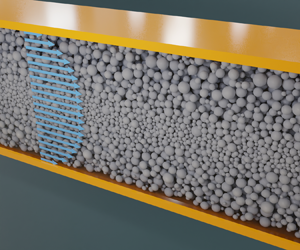
The numerical test cell depicted in figure 1 is implemented to study granular particle bulk migration and size segregation. Spheres ranging in radii from  $a_{min}$ to $a_{max}$ are suspended in a Newtonian fluid of constant density, $\rho$, and kinematic viscosity, $\nu =\eta _f/\rho$, and driven by an external body force, akin to a pressure gradient, $G$, in the $x$ direction of the channel. SIM occurs in the velocity gradient direction, $y$, transverse to the mean flow direction, $x$, and neutral direction, $z$. The boundaries in the $x$ and $z$ directions are periodic, while fixed wall particles of radius $a_w=a_{min}$ bound the flow in the $y$ direction in order to prevent the formation of a single particle layer at the wall, which is considered a numerical artefact of perfectly smooth walls (Yeo & Maxey Reference Yeo and Maxey2011; Chun et al. Reference Chun, Kwon, Jung and Hyun2017). The characteristic channel width, $W$, is defined as the distance between the innermost points of opposing wall spheres.

Figure 1. Schematic of the numerical channel used to study the bulk migration and size segregation of polydisperse suspensions with continuous PSDs ranging in radii from  $a_{min}$ to $a_{max}$. Wall particles are stationary with radius $a_w$. The boundaries are periodic in the $x$ and $z$ directions, while fluid is driven by a constant $G$ in the $x$ direction. Schematic is not to scale.
2.1.1. Lattice Boltzmann method
The flow of the suspending fluid is governed by the Navier–Stokes equations for Newtonian fluids,
 \begin{equation} \left. \begin{gathered} \boldsymbol{\nabla} \boldsymbol{\cdot} \boldsymbol{u} = 0,\\ \frac{\partial}{\partial t}(\rho \boldsymbol{u}) + \boldsymbol{u}\boldsymbol{\cdot}\boldsymbol{\nabla}(\rho\boldsymbol{u}) = \boldsymbol{\nabla} p + \boldsymbol{\nabla} \boldsymbol{\cdot} \rho\nu \left[\boldsymbol{\nabla}\boldsymbol{u} + (\boldsymbol{\nabla}\boldsymbol{u})^T\right] + \boldsymbol{F}, \end{gathered} \right\} \end{equation}
where  $\boldsymbol {u}$ is the macroscopic fluid velocity vector and $\boldsymbol {F}$ is the sum of the body force density.
In this study, (2.1) is solved via the lattice Boltzmann method (LBM). The LBM is based on the discrete Boltzmann equation (DBE), which itself discretises the velocity space of the Boltzmann equation into a finite set,  $\boldsymbol {c}_i=c_1,\ldots,c_Q$. The DBE is then integrated over discrete points in space, $\boldsymbol {x} + \boldsymbol {c}_i\delta _t$, and time, $t + \delta _t$, to obtain the lattice Boltzmann update equation (LBE),
 \begin{equation} f_i(\boldsymbol{x} + \boldsymbol{c}_i\delta_t, t + \delta_t) = f_i(\boldsymbol{x},t) - \frac{f_i(\boldsymbol{x},t) - f_i^{eq}(\rho,\boldsymbol{u})}{\tau} + \mathcal{F}(\boldsymbol{x},t), \end{equation}
in which the motion of the fluid is described by the propagation of fluid density distribution functions,  $f_i$, between the discrete lattice of computational nodes along the $\boldsymbol {c}_i$. In this way the LBE retains the properties of implicit integration of the DBE, but is updated via a local and explicit time-stepping scheme, allowing efficient parallelisation on CPU and GPU architectures (Łaniewski-Wołłk Reference Łaniewski-Wołłk2017). Therefore, while any immersed boundary method coupled with any fluid computational scheme can handle continuously evolving solid boundaries, it is this feature which renders the LBM suitable for large-scale DNS of particle suspensions, and has contributed to its increasing uptake over the last two decades (Kromkamp et al. Reference Kromkamp, van den Ende, Kandhai, van der Sman and Boom2006; McCullough et al. Reference McCullough, Leonardi, Jones, Aminossadati and Williams2016; Rettinger & Rüde Reference Rettinger and Rüde2018).
Equation (2.2) reflects the single relaxation parameter,  $\tau$, used in this work, which relaxes the $f_i$ towards their equilibrium values, $f_i^{eq}$, in what is known as the Bhatnagar–Gross–Krook collision operator. As the stability of the LBM decreases as $\tau \rightarrow 0.5$ and accuracy decreases for $\tau >1$ in general (Holdych et al. Reference Holdych, Noble, Georgiadis and Buckius2004), $\tau =1$ is used in the present study. Here, $G$ is incorporated via the external forcing term, $\mathcal {F}(\boldsymbol {x},t)$. Twenty-seven velocity directions on a three-dimensional lattice, commonly termed the $D3Q27$ velocity set, are utilised to eliminate spurious velocity currents which potentially arise in the $D3Q15$ and $D3Q19$ sets.
The macroscopic mass and momentum densities are recovered from the propagation of the mesoscopic  $f_i$,
 \begin{equation} \left. \begin{aligned} \rho(\boldsymbol{x},t) & = \sum_{i}{f_i(\boldsymbol{x},t)},\\ \rho\boldsymbol{u}(\boldsymbol{x},t) & = \sum_{i}{\boldsymbol{c}_i f_i(\boldsymbol{x},t)}. \end{aligned} \right\} \end{equation}
In this work,  $\nu =1\times 10^{-6}\,\textrm {m}^2\,\textrm {s}^{-1}$ is first specified, and $\delta _t$ is calculated based on,
 \begin{equation} \nu = c_s^2 \left(\tau - \frac{1}{2}\right)\frac{\delta_x^2}{\delta_t}, \end{equation}
where  $\delta _x$ is the lattice spacing. A sufficiently small $\delta _x$ for numerical accuracy, as shown in § 2.2, is selected. The lattice sound speed, $c_s$, is equal to $\sqrt {1/3}$ for the isothermal LBM on a square lattice. As with all numerical integration of fluid flows, the maximum stable velocity of the LBM is limited by the speed of information propagation. For bulk flow away from boundaries and $\tau \geq 1$, $C< c_s$ is a sufficient condition for stability, where $C=|\boldsymbol {u}|\delta _t/\delta _x$ is the Courant number. The presence of solid interfaces, however, significantly reduces the limit of this condition and consequently the selection of $G$ in this work. The inferred $\delta _t$ and resulting maximum $C/c_s$ are reported in § 2.3. For further introduction to the LBM the interested reader is referred to Kruger et al. (Reference Kruger, Kusumaatmaja, Kuzmin, Shardt, Silva and Viggen2017).
2.1.2. Discrete element method
The solid particles of the suspensions are modelled as spheres by the discrete element method (DEM) (Cundall & Strack Reference Cundall and Strack1979). The motion of each sphere,  $A$, is updated at each discrete time step by explicitly integrating Newton's laws of translational and rotational motion,
 \begin{equation} \left. \begin{aligned} m_A \frac{{\rm d}\boldsymbol{u}_A}{{\rm d}t} & = \sum_{B}\left(\boldsymbol{F}_{c,AB}\right) + \boldsymbol{F}_{h,A},\\ I_A \frac{{\rm d}\boldsymbol{\omega}_A}{{\rm d}t} & = \sum_{B}\left(a\boldsymbol{n} \times \boldsymbol{F}_{c,AB}\right), \end{aligned} \right\} \end{equation}
via a velocity Verlet algorithm, where  $\boldsymbol {F}_{c,AB}$ is the force on $A$ due to collision with another contacting sphere, $B$. Here, $\boldsymbol {F}_{h,A}$ is the total hydrodynamic force acting on $A$, which is directly calculated by the LBM-DEM coupling method presented in § 2.1.3. No hydrodynamic torque is transmitted to the particles.
The soft sphere interaction model on which the DEM is based replicates particle deformation by allowing the non-deforming spheres to overlap and  $\boldsymbol {F}_{c,AB}$ is then calculated as a spring-damper system, based on the sphere–sphere overlap, $\bar {x}$, and relative interaction velocity, $\bar {u}$,
 \begin{equation} \boldsymbol{F}_{c,AB} = \left(k_n\bar{x}_{n} - \gamma_n \bar{u}_{n} \right) + \left(k_t\bar{x}_{t} - \gamma_t \bar{u}_{t} \right), \end{equation}
in which the subscripts  $n$ and $t$ denote the normal and tangential components, respectively. The elastic and damping constants, $k$ and $\gamma$, are modelled in this work via Hertz contact theory, for which full expressions can be found in Kloss et al. (Reference Kloss, Goniva, Hager, Amberger and Pirker2012). In § 2.2, when the model is validated for SIM of monodisperse suspensions, $k$ and $\gamma$ are tuned by varying the coefficient of friction and coefficient of restitution. These values of $k$ and $\gamma$ are then held constant to produce the subsequent results in this work.
The maximum DEM time step for linear collisions,
 \begin{equation} \delta_{t,{DEM,max}} = \frac{2}{\omega_c}\left(\sqrt{1+\zeta^2}-\zeta\right), \end{equation}
provides a guiding criterion for DEM stability, where  $\omega _c=\sqrt {k_n/m_{min}}$ is the maximum contact natural frequency and $\zeta =\gamma /(2m_{min}\omega _c)$ is the maximum damping ratio. Equation (2.7), however, neglects the nonlinearity of the Hertz contact model, the additional damping provided by the fluid, as well as the dependence on $\bar {u}$ for large $\bar {u}$ (Burns, Piiroinen & Hanley Reference Burns, Piiroinen and Hanley2019). Consequently, a safety factor of approximately 0.1 is typically applied if selecting $\delta _t$ based on $\delta _{t,{DEM}}$ (Han, Feng & Owen Reference Han, Feng and Owen2007). In the present work, however, selecting $\delta _t$ based on $\nu$ and $\delta _x$ (as described in § 2.1.1) and utilising $\delta _{t,{DEM}}=\delta _t$ is sufficient to maintain stability for the range of simulated $G$. The selected $\delta _x$ and inferred $\delta _t$ are reported in § 2.3.
2.1.3. Fluid–solid coupling
To determine the hydrodynamic force contribution from the LBM to the DEM, and vice versa, a coupling method is required. The present model employs the partially saturated method (PSM) (Noble & Torczynski Reference Noble and Torczynski1998), which falls under the bounce-back (BB) family of LBM boundary schemes. However, the PSM differs from simpler BB schemes in that solid objects are mapped directly to the underlying lattice, with no staircase approximation or interpolation between lattice nodes. The proportion of momentum exchange with each LBM node is instead calculated by overlaying the DEM spheres with the lattice elements and calculating the solid coverage,  $\varepsilon$, at each lattice element for each time step, illustrated in two-dimensions by figure 2. Then, $\varepsilon$ is converted to the $\tau$-dependent solid weighting function originally presented by Noble & Torczynski (Reference Noble and Torczynski1998),
 \begin{equation} \beta(\tau) = \frac{\varepsilon(\tau-0.5)}{(1-\varepsilon)+(\tau-0.5)}, \end{equation}
which is applied to (2.2) to obtain a modified LBE,
 \begin{equation} f_i(\boldsymbol{x} + \boldsymbol{c}_i\delta_t, t + \delta_t) = f_i(\boldsymbol{x},t) - \left(1-\beta\right)\frac{f_i(\boldsymbol{x},t) - f_i^{eq}(\rho,\boldsymbol{u})}{\tau} + \mathcal{F}(\boldsymbol{x},t) + \beta\varOmega_i^S, \end{equation}
where  $\varOmega _i^S$ is a new ‘solid’ collision operator. This work employs the non-equilibrium BB form,
 \begin{equation} \varOmega_i^S = f_{{-}i}(\boldsymbol{x},t) - f_i(\boldsymbol{x},t) + f_i^{eq}(\rho,\boldsymbol{u}_s) - f_{{-}i}^{eq}(\rho,\boldsymbol{u}), \end{equation}
due to its superior convergence and accuracy over other operators in permeability tests (Wang, Leonardi & Aminossadati Reference Wang, Leonardi and Aminossadati2018). The subscript  $-i$ denotes the bounced-back direction, and $\boldsymbol {u}_s$ is the weighted average velocity of all solid objects mapped to the lattice node.

Figure 2. Mapping of DEM spheres to the LBM lattice elements and calculation of the solid coverage,  $\varepsilon$, at each lattice element for the PSM.
The hydrodynamic force imparted by the fluid on particle  $A$ is conveniently calculated by summing contributions of the $\varOmega _i^S$ from all of the lattice elements, $\psi$, which map $A$ to the underlying grid,
 \begin{equation} \boldsymbol{F}_{h,A} = \frac{\delta_x^2}{\delta_t} \sum_{\psi} \left(\varepsilon_{\psi}\sum_i\varOmega_i^S\boldsymbol{c}_i\right). \end{equation}
Overall, the PSM effectively interpolates the boundary to calculate the weighted momentum exchange between the fluid and each solid object, while dependence on  $\tau$ in maintained. Compared with standard BB, however, which is first-order accurate, the PSM maintains the second-order accuracy of the LBM (Strack & Cook Reference Strack and Cook2007). Further, unlike interpolating methods, it is local, mass conserving and, as all nodes are treated as fluid nodes and information is retained, newly uncovered or covered nodes do not need to be specially treated. Consequently, the PSM has successfully been applied in simulations of dense suspensions across a range of applications (Cook, Noble & Williams Reference Cook, Noble and Williams2004; Owen, Leonardi & Feng Reference Owen, Leonardi and Feng2011; Yang et al. Reference Yang, Jing, Kwok and Sobral2019), and the exact two-way momentum exchange (within second-order accuracy) makes it an excellent candidate to resolve SIM. Implementation of the PSM is achieved via coupling of the open source LBM code base TCLB (Łaniewski-Wołłk & Rokicki Reference Łaniewski-Wołłk and Rokicki2016) and DEM solver LIGGGHTS (Kloss et al. Reference Kloss, Goniva, Hager, Amberger and Pirker2012).
2.2. Verification and validation
The theoretical second-order numerical accuracy of the PSM is verified via the benchmark case of a single sphere settling between two infinite parallel plates. Initialised at a quarter of the distance between the two plates, the sphere is allowed to settle under the influence of gravity until it reaches a terminal settling velocity due to the inhibiting drag from the plates. The flow around the sphere remains in the Stokes regime. Diffusive scaling is applied to the spatial and temporal resolutions (i.e.  $\delta_t \propto \delta_x^2$), which maintains identical physical viscosity between tests in accordance with (2.4). Figure 3 plots the error between the measured terminal velocities for each $\delta _x$ and the analytical solution (Faxen Reference Faxen1923), demonstrating second-order convergence with increasing lattice resolution. The lattice nodes per sphere radius, $a/\delta _x$, range from five for the lowest resolution up to 20 for the highest resolution, corresponding to an error range relative to the analytical solution of $0.009$– $0.2$.

Figure 3. Log–log plot demonstrating the second-order (dashed line) convergence of the present LBM-DEM model.
Following the model's numerical verification, its ability to accurately capture SIM is validated via comparison with benchmark experimental (Lyon & Leal Reference Lyon and Leal1998a) and recent LBM-DEM (Chun et al. Reference Chun, Kwon, Jung and Hyun2017) modelling, as well as the analytical DFM result, for a simple test case comprising monodisperse spheres of radius  $a$. The case parameters are set to $\bar {\phi }=0.4$ and $W/a=44.6$, with periodic dimensions of $X/a=17.1$ and $Z/a=11.4$, closely emulating the literature studies. A lattice resolution resulting in $a/\delta _x=5.6$ is utilised. From this validation case, the friction and restitution coefficients of the DEM Hertz contact model are tuned to values of 0.5 and 0.8, respectively.
In figure 4 both  $\phi$ and the suspension velocity, $u$, normalised by the mean suspension velocity, $\langle u \rangle$, are plotted at points across the channel, $y$, normalised by the channel width. Overall, the characteristic concentration profile peak and blunted velocity profile are resolved by the present model. The concentration profile is smoother and adheres to the analytical DFM solution more closely compared with the prior LBM work, especially at increasing distance from the channel centre. The concentration depletion at the channel walls seen in the literature LBM results is attributed to measurement of the channel width from 0.25 $a_w$ within the wall particles. In this study the channel wall is measured from the edge of the wall particles, however, similar concentration depletion occurs if the width plane of reference is extended. Depletion in the experimental results is most likely due to wall roughness. The velocity profile shows close agreement with the literature results but is slightly more blunt. It should also be noted that the experimental results were obtained in the Stokes regime ( ${\textit {Re}}_{p,{LL}}=1.5\times 10^{-6}$), while the prior and present LBM results were obtained at ${\textit {Re}}_{p,{LL}}=1.9\times 10^{-4}$ and $1.4\times 10^{-3}$ respectively. This indicates that SIM dominates IM at $\bar {\phi }=0.4$. Here, the particle Reynolds number is calculated based on the definition in Lyon & Leal (Reference Lyon and Leal1998a), ${\textit {Re}}_{p,{LL}} = 16 \rho a^3 \langle u \rangle /(3\eta _f W^2)$, to allow comparison. An alternative definition of the particle Reynolds number incorporates the local shear rate, which is more indicative of the shear-induced self-diffusivity (Kromkamp et al. Reference Kromkamp, van den Ende, Kandhai, van der Sman and Boom2005).

Figure 4. Validation of SIM for monodisperse suspensions using the presented LBM-DEM model. Comparison of present model with literature LBM, DFM (Chun et al. Reference Chun, Kwon, Jung and Hyun2017) and experimental (Lyon & Leal Reference Lyon and Leal1998a) results, as well as pure fluid analytical case, for (a) particle concentration profile and (b) velocity profile.
Finally, fundamental cases from the works of Lyon & Leal (Reference Lyon and Leal1998b) and Chun et al. (Reference Chun, Park, Jung and Won2019) are reproduced and compared here in order to validate the segregation of particles by size in the present model. These studies were the natural extensions to bidisperse suspensions of their respective prior monodisperse SIM studies (Lyon & Leal Reference Lyon and Leal1998a; Chun et al. Reference Chun, Kwon, Jung and Hyun2017). Both literature studies were at bulk solid volume fraction of  $\bar {\phi }=0.3$, however, the experimental results (Lyon & Leal Reference Lyon and Leal1998b) were obtained at $a_L/a_S=3.4$ and $\bar {\phi }_S/\bar {\phi }=0.25$, while the numerical LBM and DFM results (Chun et al. Reference Chun, Park, Jung and Won2019) were obtained at $a_L/a_S=1.9$ and $\bar {\phi }_S/\bar {\phi }=0.33$. Figure 5 compares the results obtained by the present model with both the experimental and numerical literature results. The parameters used to obtain the present model results match the parameters of their respective literature comparison studies, and as such the present model results of figures 5(a) and 5(b) are quantitatively different. Concentration profiles are shown for half of the channel ( $0< y/W<0.5$) for clarity. Excellent agreement with Lyon & Leal (Reference Lyon and Leal1998b) and Chun et al. (Reference Chun, Park, Jung and Won2019) is seen for the concentration of large particles, which attain a maximum concentration in the centre of the channel and a minimum at the channel walls. Small particles, on the other hand, maintain a relatively uniform concentration across the channel, with the present model obtaining a slightly higher concentration at the wall compared with both the experimental and numerical results. It must be noted that all results in figure 5 are obtained at $L/W=560$, where $L$ is the distance that the suspension has travelled based on the mean suspension velocity. This concept will be discussed further as the distances required for development of size segregation are analysed.

Figure 5. Validation of particle segregation by size for bidisperse suspensions via comparison with fundamental (a) experimental (Lyon & Leal Reference Lyon and Leal1998b) and (b) numerical LBM and DFM (Chun et al. Reference Chun, Park, Jung and Won2019) cases.
2.3. Particle distributions and parametrisation
In the present work five distinct polydisperse PSDs ( $P_1$, $P_2$, $P_3$, $P_{2,1}$, $P_{2,2}$) are implemented as the basis for investigating the effect of polydispersity on bulk migration and size segregation. The PSDs are characterised by their first three statistical moments, namely mean, variance and skewness, here denoted by $M_1$, $M_2$ and $M_3$, respectively. The reason for doing so is based on the fact that the rheologies of polydisperse PSDs are completely described by their first three statistical moments, and that bidisperse and polydisperse distributions with matching $M_1$, $M_2$ and $M_3$ have identical effective viscosity (Pednekar et al. Reference Pednekar, Chun and Morris2018). In this work the bidisperse–polydisperse equivalence is shown to extend to SIM in pressure-driven Poiseuille flows.
A two-parameter Weibull function is used to define the probability density functions,  $f(a)$, of the number of particles by particle size,
 \begin{equation} f(a) = \frac{\lambda_1}{\lambda_2}\left(\frac{a}{\lambda_2}\right)^{\lambda_1-1}e^{-\left(a/\lambda_2\right)^{\lambda_1}}. \end{equation}
The shape and scale parameters,  $\lambda _1$ and $\lambda _2$, consequently define $M_1$, $M_2$ and $M_3$. The statistical measurements of all PSDs are reported in table 1, which also includes $\phi _{rcp}$ as calculated from an empirical formula based on the statistical moments (Desmond & Weeks Reference Desmond and Weeks2014),
 \begin{equation} \phi_{rcp} = \phi^*_{rcp} + c_1\frac{\sqrt{M_2}}{M_1} + c_2 \frac{M_2 M_3}{M_1^2}, \end{equation}
where  $\phi ^*_{rcp}$ is the maximum random close packing concentration for monodisperse spheres and $c_1=0.0658$ and $c_2=0.0857$ are empirically determined coefficients. $P_1$, $P_2$ and $P_3$ are designed to have widely varying $M_1$, $M_2$, $M_3$, and consequently $\phi _{rcp}$, while $P_2$, $P_{2,1}$ and $P_{2,2}$ have matching $M_1$ but significantly different $M_2$, $M_3$ and $\phi _{rcp}$, in order to isolate any dependence on $M_1$. Figure 6 plots the $f(a)$ of all PSDs, while figure 7 re-plots the $f(a)$ as the bulk concentration of each particle size, $\bar {\phi }_j$, rather than the number of particles, to give a more meaningful volumetric interpretation when analysing bulk migration and size segregation.
Table 1. Statistical measurements of the five polydisperse PSDs used in this work. The Weibull parameters,  $\lambda _1$ and $\lambda _2$, define the distributions, which are subsequently characterised by their first three statistical moments, $M_1$, $M_2$ and $M_3$, and the random close packing solid volume fraction, $\phi _{rcp}$.


Figure 6. Probability density functions for the five different PSDs tested.

Figure 7. Concentration by particle size of each PSD. Note that  $\bar {\phi }_j$ scales arbitrarily.
The PSDs are shifted such that  $a_{min}=1\,\mathrm {\mu }\textrm {m}$, and truncated at a maximum of $a_{max}=3.9\,\mathrm {\mu }\textrm {m}$, such that $a_{max}/a_{min}=3.9$. It is acknowledged that Brownian and electrostatic forces could influence results at these particle sizes, however, this is considered outside the scope of the present work. It is also noted that, in the absence of these forces, it is not essential to designate physical length scales to the particles, however, this is done in this work as a matter of style and to increase the ease of interpretation and discussion of the results.
The continuous distributions of particle radii are implemented in the DEM as discrete radii, but in sufficiently small increments of  $\delta _a=0.1\,\mathrm {\mu }\textrm {m}$ so as to closely approximate a continuous distribution. Particle species are defined by particle size, such that all particles comprising a single particle size are designated as a single species, $j$. With $[a_{min},a_{max}]=[1,3.9]\,\mathrm {\mu }\textrm {m}$ and $\delta _a=0.1\,\mathrm {\mu }\textrm {m}$ there are a total of $K=30$ particle size species.
As well as varying the PSDs,  $\bar {\phi }$ is varied between 0.2 and 0.55. $G$ is varied between 1 and $16\,\textrm {MPa}\,\textrm {m}^{-1}$ in order to analyse the competing effects of SIM and IM, and to maintain ${\textit {Re}}_c$ in the cases where $\bar {\phi }$ is varied. The degree of inertia is defined by the channel Reynolds number,
 \begin{equation} {\textit{Re}}_c = \frac{\rho \langle u \rangle W}{\bar{\eta}_s} = \frac{12 \rho \langle u \rangle^2}{GW}, \end{equation}
where  $\langle u \rangle$ is the mean channel suspension velocity. The bulk effective shear viscosity, $\bar {\eta }_s$, is distinguished from the local effective shear viscosity, $\eta _s(\phi )$, as the latter varies locally with the particle size composition. There is no single way to define the channel bulk effective shear viscosity; here $\bar {\eta }_s = GW^2/(12\langle u \rangle )$ is used, analogous to momentum conservation for planar Poiseuille flow.
The numerical domain is held constant for all tests at  $W=100\,\mathrm {\mu }\textrm {m}$, $X=64\,\mathrm {\mu }\textrm {m}$ and $Z=38\,\mathrm {\mu }\textrm {m}$. A domain dependence study was performed prior to determining these dimensions, showing that migration is independent of the domain height for $Z\geq 20\,\mathrm {\mu }\textrm {m}$. A lattice spacing of $\delta _x=0.4\,\mathrm {\mu }\textrm {m}$ is utilised, corresponding to $a_{min}/\delta _x=2.5$ and $a_{max}/\delta _x=9.75$. According to (2.4), the inferred $\delta _t=\delta _{t,{DEM}}$ is therefore $2.667\times 10^{-8}\,\textrm {s}$, resulting in $C/c_s \leq 0.233$ and $\delta _{t,{DEM}}/\delta _{t,{DEM,max}} \approx 0.2$ (for linear collisions according to (2.7)).
It must also be noted that, between parametrically and statistically identical simulations and distributions with different randomised particle injections, there is appreciable difference in bulk migration and size segregation between the simulations. This reflects the stochastic nature of the accumulated irreversible particle interactions which contribute to SIM. These differences, however, average over all simulations. As such, in some cases the data points are the median of up to ten simulations with randomised injection between each.
3. Results
The degree of SIM of particles of a particular size (i.e. those comprising particle species  $j$) is conveniently measured by the scalar dispersion function,
 \begin{equation} C_j(t) = \frac{1}{N_j}\sum_{i=1}^{N_j} \left| \frac{y_i}{w} - \frac{1}{2} \right|, \end{equation}
where  $N_j$ is the number of particles of species $j$ and $y_i$ is the transverse ordinate of the $i$th particle in species $j$. Overall, $C_j$ is the distance from the mid-plane averaged over all particles of species $j$ at each time step. $C_j=0$ if all particles are positioned exactly in the middle of the channel, while $C_j=0.5$ if all particles are positioned exactly on the channel walls. It is defined for planar flows only under the assumption that the concentration distribution is approximately symmetric about the mid-plane.
The bulk scalar dispersion function,
 \begin{equation} C(t) = \frac{\sum_{j=1}^{K} C_j \bar{\phi}_j}{\bar{\phi}}, \end{equation}
is calculated by weighting the  $C_j$ of each species by their bulk solid volume fraction, $\bar {\phi }_j$. Due to this weighting, $C$ represents the total dispersion of mass across the channel. $C \rightarrow 0$ denotes the channel-averaged particle mass approaching the mid-plane.
To quantify the relative transverse motion of particles of different sizes, and capture the difference in transient behaviour between total and relative particle motion seen in previous bidisperse studies, a scalar segregation function is also defined,
 \begin{equation} C_\varSigma(t) = \frac{4}{K}\sum_{i=1}^K\left(\frac{1}{K}\sum_{j=1}^K|C_i-C_j|\right), \end{equation}
which takes into account the difference in channel position between particles of all sizes. It is constructed in such a way that, if all particle sizes are distributed in the same manner,  $C_\varSigma =0$. If all particles representing half of the size species are positioned in the channel centre, and all particles of the other half of size species are at the channel wall, $C_\varSigma$ attains a maximum value of 1.
The primary scale of interest is the mean length travelled along the channel,  $L$, by the suspension. Due to the discrete nature of the numerical model it may be calculated at each time step,
 \begin{equation} L(t) = \sum_{i=0}^t \langle u \rangle _i \Delta t, \end{equation}
and is expressed throughout the results relative to the channel width,  $L/W$.
3.1. Distribution (polydispersity)
The SIM of the five continuous PSDs are firstly compared, at constant parameters of  $\bar {\phi }=0.3$ and $G=2\,\textrm {MPa}\,\textrm {m}^{-1}$, to investigate the effect of polydispersity on bulk migration and size segregation. This combination of $\bar {\phi }$ and $G$ results in ${\textit {Re}}_c \approx 25$ across all simulations for all PSDs (at $L/W\approx 1800$).
Firstly, the transient development of  $C$ depicted in figure 8 suggests that the bulk migration for each PSD reaches steady state after $L/W\approx 600$. The lowest steady state $C$ achieved by $P_3$ indicates that a higher volume of particles have accumulated at the channel centre, compared with all other PSDs. In other words, the suspension with the highest mean particle size ( $P_3$) has attained the highest degree of bulk migration by particle volume, while the suspension with the lowest mean ( $P_1$) has the most spread particle concentration. While the suspensions with matching mean ( $P_2$, $P_{2,1}$, $P_{2,2}$) have closer $C$ compared with $P_1$ and $P_3$, their distinct difference indicates that bulk migration is also a function of the variance and skewness ( $M_2$ and $M_3$), but to a lesser degree than the mean ( $M_1$).

Figure 8. Development of bulk scalar dispersion function,  $C$, along normalised channel length, $L/W$. Comparison of each PSD at $\bar {\phi }=0.3$, $G=2\,\textrm {MPa}\,\textrm {m}^{-1}$. Lower $C$ indicates that the channel-averaged particle mass is closer to the channel mid-plane.
The scalar bulk migration in figure 8 is commensurate with the plot of concentration profiles for  $P_1$, $P_2$ and $P_3$ in figure 9. It is clear that $P_3$ has a higher particle concentration around the centre of the channel ( $0.4 < y/W < 0.6$), but lower at the edges ( $y/W < 0.2$, $y/W > 0.8$), compared with $P_2$ and $P_1$. The concentration plots for $P_{2,1}$ and $P_{2,2}$ are omitted from figure 9 on the grounds that they closely match that of $P_2$, as their bulk migration is similar. Compared with the concentration profile for the monodisperse case in figure 4, the polydisperse suspensions attain significantly sharper concentration peaks which drop away much more at the channel walls. The decreased wall concentration is due to two factors. Firstly, particles become less uniformly distributed near the walls as $W/a$ decreases (Kazerooni et al. Reference Kazerooni, Fornari, Hussong and Brandt2017), and the ratio of $W/a_{max}$ is relatively low in this work. Secondly, interactions with wall particles cause a depletion of the particle concentration near the wall. While decreasing the wall particle size would decrease this depletion effect, at the limit of $a_w \rightarrow 0$ the virtually smooth wall would cause a single layer of wall particles to form which is non-physical. In a similar vein a realistic surface roughness, especially of naturally occurring fractures, is self-affine and comprises a range of wavelengths, posing the question of what size is representative (Łaniewski-Wołłk & Leonardi Reference Łaniewski-Wołłk and Leonardi2020). The scope of this investigation is narrowed by cutting the spectrum of the roughness to wavelengths equal or lower than the smallest particle size, by setting $a_w = a_{min}$. Analysis of varying $a_w$ merits further investigation, but is outside the scope of the current work.

Figure 9. Concentration profiles plotted as solid volume fraction,  $\phi$, across the normalised channel width, $y/W$. Comparison of $P_1$, $P_2$ and $P_3$ at $\bar {\phi }=0.3$, $G=2\,\textrm {MPa}\,\textrm {m}^{-1}$, with measurements taken at $L/W\approx 1800$.
Blunting of the velocity profiles, which is also characteristic of SIM, is demonstrated in figure 10. Unlike the concentration profiles, there is negligible dependence on the PSD for the velocity profiles. This lack of variation due to concentration by particle size is in line with prior bidisperse results (Lyon & Leal Reference Lyon and Leal1998b; Chun et al. Reference Chun, Park, Jung and Won2019). The slip velocity immediately adjacent to the walls is due to the wall depletion interaction just described.

Figure 10. Velocity profile plotted as channel velocity,  $u$, normalised by mean channel velocity, $\langle u\rangle$. Comparison of $P_1$, $P_2$ and $P_3$ at $\bar {\phi }=0.3$, $G=2\,\textrm {MPa}\,\textrm {m}^{-1}$, with measurements taken at $L/W\approx 1800$.
To analyse the size segregation between individual size species, figure 11 shows  $C_j$ over the full range of particle sizes measured at $L/W\approx 1800$. It must first be noted that, while particle sizes are implemented in the DEM in discrete increments of $\delta _a=0.1\,\mathrm {\mu }\textrm {m}$, $C_j$ is plotted here in particle bins of width $a=0.4\,\mathrm {\mu }\textrm {m}$. This is primarily done for ease of interpretation and visualisation. Further, the stochastic nature of SIM results in variation of bulk migration and size segregation between parametrically identical simulations, as explained in § 2.3. Consequently, only the median values of $C_j$ are included. A full box and whisker plot showing the variability in the data over all randomised simulations is shown in the Appendix.

Figure 11. Scalar dispersion function by particle size species,  $C_j$. Comparison of each PSD at $\bar {\phi }=0.3$, $G=2\,\textrm {MPa}\,\textrm {m}^{-1}$, with measurements taken at $L/W\approx 1800$. Particles are grouped into bins by radius of width $0.4\,\mathrm {\mu }\textrm {m}$, recalling that $\delta _a=0.1\,\mathrm {\mu }\textrm {m}$, and are plotted at their median value, $\langle a \rangle$. Lower $C_j$ indicates particles have migrated closer to the channel mid-plane.
Two significant observations can be made from figure 11. Firstly, for all PSDs, the largest particles do not migrate most to the channel centre relative to all particle sizes. This is especially pronounced for  $P_1$ and $P_{2,2}$, for which the particles of size $2.5 \leq a \leq 2.9\,\mathrm {\mu }\textrm {m}$ attain the highest occupancy at the channel centre. If interpreted via a concentration profile plot, these particles would exhibit a larger peak at the channel centre compared with the largest particles. Secondly, the migration of individual particle sizes differs significantly between PSDs, with this difference being especially pronounced for $P_{2,1}$ and $P_{2,2}$.
The results presented thus far can be analysed in terms of the classical homogeneous rheology description of SIM: as described in § 1, the bulk migration and size segregation of polydisperse suspensions depend on both the particle self-diffusivity and viscous suspension reordering. Due to scaling of the self-diffusivity (granular temperature) with particle size, larger particles will preferentially migrate to the channel mid-plane, however, their migration will be constrained by the local rheological requirements imposed by the particle pressure gradient.
The strong dependence of bulk migration on  $M_1$, for example, is obviously a direct result of the self-diffusivity scaling with particle size; a larger $M_1$ indicates a higher number of larger particles, and therefore greater bulk migration. The distinct (but smaller) difference in bulk migration between suspensions with matching $M_1$, however, also indicates a (smaller) dependence of bulk migration on $M_2$ and $M_3$. This dependence is intrinsically linked to the size segregation differences in figure 11, which are explained by the viscous suspension reordering. Recalling that the polydisperse $\phi _{rcp}$ (and consequently $\eta _n(\phi )$) given by (2.13) is a strong function of $M_2$ and $M_3$, the local $\eta _n(\phi )$ requirement induced by the particle pressure therefore drives the local particle size composition. For $P_{2,2}$, for example, in order to satisfy the viscosity at every point across the channel width, the few particles of size $3.5 \leq a \leq 4\,\mathrm {\mu }\textrm {m}$ must necessarily migrate away from the mid-plane. Conversely, $P_{2,1}$ contains a comparatively higher concentration of the largest particles, which are therefore free to attain a position closest to the mid-plane, while the smallest particles must be more spread.
Confirmation of this hypothesis requires interrogation of the particle pressure to obtain the self-diffusivity of individual size species and the overall particle pressure gradient, as well as the use of an adequate model of the local suspension rheology. Due to its complexity, however, this type of analysis is left for a future work which may seek to exactly quantify particle diffusion in relation to polydispersity.
To analyse the transient size segregation in greater depth, figure 12 plots the development of  $C_j$ along the channel, separated into the same particle bins of width $a=0.4\,\mathrm {\mu }\textrm {m}$ as in figure 11, for $P_1$, $P_2$ and $P_3$. What emerges is a very different transient response compared with $C$ alone. Most notably, for all three PSDs, the largest particles ( $3.5 \leq a \leq 3.9\,\mathrm {\mu }\textrm {m}$) exhibit an initial SIM to a minimum $C_j$, evidently driven by the self-diffusivity (which scales with particle size). After this initial SIM, however, the largest particles reverse their overall SIM direction (i.e. $C_j$ begins to increase) and they begin to migrate back towards the channel walls due to the viscous suspension reordering. It follows that this reordering of the local particle composition, and hence the long-term size segregation, occurs on a longer time scale than the particle diffusion.

Figure 12. Transient development of scalar dispersion function by particle size species,  $C_j$. Comparison of (a) $P_1$, (b) $P_2$ and (c) $P_3$ at $\bar {\phi }=0.3$, $G=2\,\textrm {MPa}\,\textrm {m}^{-1}$. Particles are grouped into bins by radius of width $0.4\,\mathrm {\mu }\textrm {m}$, recalling that $\delta _a=0.1\,\mathrm {\mu }\textrm {m}$. Labels on lines indicate bin size in $\mathrm {\mu }\textrm {m}$. Markers represent the bulk scalar dispersion of the suspensions, $C$. Lower $C_j$ and $C$ indicates particles have migrated closer to the channel mid-plane.
The transient size segregation development is also reflected in the scalar segregation function. The values of  $C_{\varSigma }$ in figure 13, are commensurate with the trends of $C_j$ for individual particle size species in figure 12. For $P_1$, $C_{\varSigma }$ reaches a maximum at $L/W\approx 400$, which coincides with the reversal of the largest particles in figure 12(a). The value of $C_{\varSigma }$ then slowly decreases, never reaching a clear steady state, which corresponds to the slow increase of $C_j$ of the largest particles. For $P_2$, on the other hand, $C_{\varSigma }$ appears to reach a constant value at $L/W \approx 800$, which is also evident in figure 12(b). As $P_3$ is composed mainly of larger particles, a trend in $C_{\varSigma }$ is harder to distinguish, however, it could reasonably be concluded in conjunction with figure 12(c) that steady state is reached at $L/W \approx 600$. Overall, viscous suspension reordering occurs on a longer time scale for suspensions containing a larger proportion of smaller particles. These reordering/segregation development lengths also correspond to a range of 1.3–3 times larger than the development lengths for suspension bulk migration. This range of time scale differences is much lower than that previously observed for bidisperse suspensions (Chun et al. Reference Chun, Park, Jung and Won2019).

Figure 13. Development of scalar segregation function,  $C_\varSigma$, along the normalised channel length, $L/W$, highlighting the transient size segregation behaviour of polydisperse suspensions. Comparison of $P_1$, $P_2$ and $P_3$ at $\bar {\phi }=0.3$, $G=2\,\textrm {MPa}\,\textrm {m}^{-1}$. Higher $C_\varSigma$ indicates greater size segregation.
3.2. Concentration
The following results investigate the effect of bulk suspension concentration,  $\bar {\phi }$, on particle SIM in polydisperse suspensions. Firstly, concentrations of $\bar {\phi }=0.2,$ 0.3, 0.4 and 0.5 are tested for $P_2$ only. The pressure gradient is increased with $\bar {\phi }$ as $G=1.1,$ 2, 4.25 and $10\,\textrm {MPa}\,\textrm {m}^{-1}$ in order to obtain a similar ${\textit {Re}}_c$ for all $\bar {\phi }$ ( ${\textit {Re}}_c=25,$ 25, 25 and 20). The lower value of ${\textit {Re}}_c=20$ for $\bar {\phi }=0.5$ is the maximum achievable ${\textit {Re}}_c$ while maintaining numerical stability. In § 3.3, however, this small inertial difference is shown to have negligible impact on SIM at $\bar {\phi }=0.5$.
Figures 14 and 15 summarise the effect of suspension concentration on bulk migration and size segregation. According to figure 14, at the lowest concentration ( $\bar {\phi }=0.2$) bulk migration is low (i.e. $C$ is high). There is still size segregation, as shown in the variation of $C_j$ for different particle sizes in figure 15, but the values of $C_j$ are slightly higher compared with $\bar {\phi }=0.3$. In figure 14, bulk migration is similar for $\bar {\phi }=0.3$ and $\bar {\phi }=0.4$, however, as the concentration is further increased to $\bar {\phi }=0.5$, $C$ significantly increases again, suggesting that there is a critical bulk concentration at $\bar {\phi }\approx 0.3- 0.4$ where a change in behaviour occurs. Figure 15 shows that at this change in behaviour the larger particles migrate closer to the channel walls, relative to smaller particles. This is accentuated as $\bar {\phi }$ increases. For $\bar {\phi }=0.4$, particles of size $2 \leq a \leq 2.4\,\mathrm {\mu }\textrm {m}$ migrate closest to the channel centre, while for $\bar {\phi }=0.5$ particles of size $1 \leq a \leq 1.9\,\mathrm {\mu }\textrm {m}$ migrate closest to the channel centre. Figure 16 illustrates this phenomenon, which has not been reported in the literature for dense suspensions hitherto.

Figure 14. Development of bulk scalar dispersion function,  $C$, along normalised channel length, $L/W$. Comparison of different $\bar {\phi }$ for $P_2$. Lower $C$ indicates that the channel-averaged particle mass is closer to the channel mid-plane.

Figure 15. Scalar dispersion function by particle size species,  $C_j$. Comparison of different $\bar {\phi }$ for $P_2$, measured at $L/W\approx 1800$. Particles are grouped into bins by particle radius of width $0.4\,\mathrm {\mu }\textrm {m}$, recalling that $\delta _a=0.1\,\mathrm {\mu }\textrm {m}$, and are plotted at their median value, $\langle a \rangle$. Lower $C_j$ indicates particles have migrated closer to the channel mid-plane.

Figure 16. Graphical representations of (a)  $\bar {\phi }=0.4$ $z$-plane, (b) $\bar {\phi }=0.5$ $z$-plane, (c) $\bar {\phi }=0.5$ isometric, captured at $L/W\approx 1800$ for $P_2$.
The velocity profiles for each  $\bar {\phi }$ are plotted in figure 17. Total flattening of the velocity profiles for $\bar {\phi }=0.4$ and 0.5 indicate the regions in which a plug has formed (i.e. $\phi$ has reached $\phi _m$ such that the shear rate vanishes). A large plug spanning 1/5 of the channel width forms for $\bar {\phi }=0.5$, while a smaller one forms for $\bar {\phi }=0.4$. These are indicated on the velocity profiles with vertical dashed and dotted lines, respectively. This plug formation at $\bar {\phi }=0.4$ coincides with the change in behaviour elucidated above.

Figure 17. Comparison of velocity profiles for increasing  $\bar {\phi }$ for $P_2$, measured at $L/W\approx 1800$. Plugged regions are indicated by vertical dotted lines for $\bar {\phi }=0.4$ and vertical dashed lines for $\bar{\phi}=0.5$.
It is evident that the plugs first form due to bulk migration, and preferentially comprise the smallest sized particles. This then determines which particles compose the sheared region outside the plug, where  $\dot {\gamma }>0$. The larger the plug, the more small particles are required to compose the plug, meaning that more large particles will be closer to the channel walls (i.e. the $C_j$ of large particles, as well as the overall $C$, will gradually increase as the plug size increases). Figure 18 illustrates how the small particles segregate to form the plugs, and that the length scale on which this size segregation occurs increases significantly as $\bar {\phi }$ increases.

Figure 18. Transient development of scalar dispersion function by particle size species,  $C_j$, for (a) $\bar {\phi }=0.4$ and (b) $\bar {\phi }=0.5$. Particles are grouped into bins by radius of width $0.4\,\mathrm {\mu }\textrm {m}$, recalling that $\delta _a=0.1\,\mathrm {\mu }\textrm {m}$. Labels on lines indicate bin size in $\mathrm {\mu }\textrm {m}$. Markers represent the bulk scalar dispersion of the suspensions, $C$. Lower $C_j$ indicates particles have migrated closer to the channel mid-plane.
Preferential formation of the plugs with small particles can be explained in terms of particle fluctuations, which propagate into the plug (where  $\dot {\gamma }=0$) from just inside the sheared region (where $\dot {\gamma }>0$), causing particle rearrangements to persist (Lecampion & Garagash Reference Lecampion and Garagash2014). In the plugged region, particle motions are completely defined by the amplitude of the root mean square of shear-rate fluctuations, $\dot {\gamma }_{rms}$ (Gillissen & Ness Reference Gillissen and Ness2020). As $\dot {\gamma }_{rms}$ scales inversely with the particle size ( $\dot {\gamma }_{rms} \propto \sqrt {T}/a$), it is the small particles which have the greatest motion within the plug (Pähtz et al. Reference Pähtz, Durán, de Klerk, Govender and Trulsson2019). Consequently, as the plug forms, it is the smallest particles which will preferentially fluctuate to within the plug. Less formally, based on a simple momentum conservation view, the fluctuation propagation from the sheared region must cause the smaller particles to rebound towards the channel mid-plane with a greater velocity. Consequently, as the plug grows, it is the smaller particles which will be continually forced ahead of the larger particles and into the plug.
Although not explicitly shown here, these phenomena occur for all PSDs at  $\bar {\phi } \geq 0.4$. An additional observation in figure 19 is that, as $\bar {\phi }$ increases, bulk migration becomes independent of the particle distribution (i.e. the same $C$ is attained). Here, a pressure gradient of $G=16\,\textrm {MPa}\,\textrm {m}^{-1}$ is applied to $\bar {\phi }=0.55$, resulting in ${\textit {Re}}_c \approx 13$. Also plotted in figure 20 is the increase in bulk effective shear viscosity, $\bar {\eta }_s$, with $\bar {\phi }$. Comparison is made with the theoretical correlation of Krieger & Dougherty (Reference Krieger and Dougherty1959), $\eta _s/\eta _f=(1-\phi /\phi _{rcp})^{-2.5\phi _{rcp}}$, where $\phi _{rcp}$ is obtained using (2.13). This general approach of substituting an expression for the maximum packing fraction into an existing viscosity correlation has been highly successful (Pednekar et al. Reference Pednekar, Chun and Morris2018) and reproduces a dependence on the PSD. The obtained $\bar {\eta }_s$ in figure 20 exhibit this same dependence, which becomes more pronounced at higher $\bar {\phi }$. Divergence of the simulation $\bar{\eta}_{s}$ from the correlation at $\bar {\phi } \geq 0.4$ occurs as the former is a channel-averaged quantity and decreases with the presence of a plug (where the mean shear rate is zero), while the correlation is for a locally sheared suspension.

Figure 19. Development of bulk migration,  $C$, along the length of the channel, $L/W$, for (a) $\bar {\phi }=0.4$, (b) $\bar {\phi }=0.5$ and (c) $\bar {\phi }=0.55$, indicating that as $\bar {\phi }$ increases, bulk migration becomes independent of the particle distribution.

Figure 20. Increase in bulk effective shear viscosity with bulk solid volume fraction, obtained from simulations as  $\bar {\eta }_s = GW^2/(12\langle u \rangle )$. Comparison with theoretical correlation of Krieger & Dougherty (Reference Krieger and Dougherty1959), $\eta _s/\eta _f=(1-\phi /\phi _{rcp})^{-2.5\phi _{rcp}}$, where $\phi _{rcp}$ is obtained using (2.13).
3.3. Inertia
As outlined in § 1, suspension migration is dependent on a combination of IM and SIM, to varying degrees. Firstly, to quantify the contribution of inertia to the results in § 3.1,  $G$ is varied between values of 1, 2 and $3\,\textrm {MPa}\,\textrm {m}^{-1}$ for $P_2$ at $\bar {\phi }=0.3$, corresponding to ${\textit {Re}}_c=13,$ 25 and 38. Figure 21 demonstrates an increase in bulk migration towards the channel walls as ${\textit {Re}}_c$ is increased. This is commensurate with the general effect of inertia causing particles to migrate away from the channel mid-plane. Conversely, by decreasing ${\textit {Re}}_c$, IM decreases relative to SIM, causing greater bulk migration to the channel mid-plane.

Figure 21. Development of bulk scalar dispersion function,  $C$, along normalised channel length, $L/W$. Comparison of different $G$ for $P_2$ at $\bar {\phi }=0.3$, demonstrating dependence of migration on inertia at moderate $\bar {\phi }$.
Figure 22, however, shows that the largest particles attain a position closer to the channel centre as  $G$ (and hence inertia) increases, while the smallest particles migrate closer to the channel walls. This behaviour can be explained by the dependence of SIM on the particle Reynolds number, as discussed in § 1. As the particle self-diffusivity increases with ${\textit {Re}}_p$ (Kromkamp et al. Reference Kromkamp, van den Ende, Kandhai, van der Sman and Boom2005), it is the larger particles which will exhibit the greatest increase in SIM (and hence closest position to the mid-plane) with increasing $G$.
$G$.

Figure 22. Scalar dispersion function by particle size species,  $C_j$. Comparison of different $G$ at $\bar {\phi }=0.3$ for $P_2$, measured at $L/W\approx 1200$. Particles are grouped into bins by particle radius of width $0.4\,\mathrm {\mu }\textrm {m}$, recalling that $\delta _a=0.1\,\mathrm {\mu }\textrm {m}$, and are plotted at their median value, $\langle a \rangle$. Lower $C_j$ indicates particles have migrated closer to the channel mid-plane.
Next, to compare the effect of inertia at the higher solid volume fractions tested in § 3.2,  $G$ is varied between values of $G=3,$ 5.5, 8 and $10\,\textrm {MPa}\,\textrm {m}^{-1}$ for $P_2$ at $\bar {\phi }=0.5$, corresponding to ${\textit {Re}}_c=6,$ 11, 16 and 20. Figures 23 and 24 show that the variation in bulk migration and size segregation with inertia is minimal. This is commensurate with the fact that dependence of self-diffusivity on $Re_p$ disappears with higher $\bar {\phi }$, and also suggests that SIM is generally dominating IM due to the high particle concentration.

Figure 23. Development of bulk scalar dispersion function,  $C$, along normalised channel length, $L/W$. Comparison of different $G$ for $P_2$ at $\bar {\phi }=0.5$, demonstrating independence of migration on inertia at high $\bar {\phi }$.
3.4. Equivalence of bidisperse suspensions
Here, a quantitative comparison is made between the bulk migration and size segregation of bidisperse and polydisperse suspensions, motivated by the recent finding that bidisperse and polydisperse suspensions with matching first three statistical moments (mean, variance, skewness –  $M_1$, $M_2$, $M_3$) exhibit matching viscosity (Pednekar et al. Reference Pednekar, Chun and Morris2018). To assess whether this equivalence translates to SIM in channel flows, the first three statistical moments are also used here as a measure of equivalence. Table 2 defines the five bidisperse PSDs ( $B_1$, $B_2$, $B_3$, $B_{2,1}$, $B_{2,2}$) which are statistically equivalent to their respective polydisperse PSDs defined in § 2.3 ( $P_1$, $P_2$, $P_3$, $P_{2,1}$, $P_{2,2}$). Therefore, $M_1$, $M_2$ and $M_3$ exactly match those in table 1. These moments are then defined for bidisperse PSDs,
 \begin{equation} \left. \begin{aligned} M_1 & = a_S N_S + a_L(1-N_S),\\ M_2 & = N_S\left(a_S-M_1\right)^2 + (1-N_S)\left(a_L-M_1\right)^2,\\ M_3 & = \left[N_S\left(a_S-M_1\right)^3 + (1-N_S)\left(a_L-M_1\right)^3\right]/M_2^{3/2}, \end{aligned} \right\} \end{equation}
where  $a_S$ and $a_L$ are the radii of small and large particles, respectively, and $N_S$ is the number fraction of small particles. To obtain $a_S$, $a_L$ and $N_S$ the system of (3.5) are simultaneously solved for each PSD by substituting the respective values of $M_1$, $M_2$ and $M_3$ from table 2. With matching moments $\phi _{rcp}$ must also be equal according to (2.13).

Figure 24. Scalar dispersion function by particle size species,  $C_j$. Comparison of different $G$ at $\bar {\phi }=0.5$ for $P_2$, measured at $L/W\approx 1200$. Particles are grouped into bins by particle radius of width $0.4\,\mathrm {\mu }\textrm {m}$, recalling that $\delta _a=0.1\,\mathrm {\mu }\textrm {m}$, and are plotted at their median value, $\langle a \rangle$. Lower $C_j$ indicates particles have migrated closer to the channel mid-plane.
Table 2. The five bidisperse PSDs used in this work, with first three statistical moments,  $M_1$, $M_2$ and $M_3$, taken to match their respective polydisperse distributions in table 2. Equations (3.5) are then solved simultaneously to obtain the radii of small and large particles, $a_S$ and $a_L$, and the number fraction of small particles, $N_S$. Here, $\phi _{rcp}$ is obtained from (2.13).

Firstly, the five bidisperse suspensions are simulated at constant parameters of  $\bar {\phi }=0.3$ and $G=2\,\textrm {MPa}\,\textrm {m}^{-1}$ to facilitate comparison with their equivalent polydisperse suspensions. Figure 25 shows that the bulk migration of the bidisperse suspensions matches that of the polydisperse suspensions (figure 8) remarkably closely. Consequently, it may confidently be concluded that the rheological equivalence of bidisperse and polydisperse suspensions extends to SIM in channel flows. In this way, the first three statistical moments must also completely describe the shear-induced diffusivity of a suspension. By extension, this supports the theory that a classical homogeneous rheology description of SIM, such as the effective temperature SBM approach for bidisperse suspensions (van der Sman & Vollebregt Reference van der Sman and Vollebregt2012), can be extended to polydisperse suspensions, with the only requirement being adequate closure relations. It is acknowledged, however, that this result is obtained empirically, for a relatively narrow set of distributions. Consequently, generalisation remains to be shown.

Figure 25. Development of bulk scalar dispersion function,  $C$, along normalised channel length, $L/W$. Comparison of each bidisperse PSD at $\bar {\phi }=0.3$, $G=2\,\textrm {MPa}\,\textrm {m}^{-1}$, demonstrating close agreement to the bulk migration of their respective polydisperse suspensions in figure 8.
Notwithstanding these similarities, two primary differences between figures 25 and 8 are evident: firstly,  $C$ is slightly higher for the bidisperse results compared with the polydisperse, meaning slightly less bulk migration to the channel mid-plane; and secondly, the bidisperse PSDs with matching mean ( $B_2$, $B_{2,1}$, $B_{2,2}$) are all slightly closer compared with their equivalent polydisperse PSDs ( $P_2$, $P_{2,1}$, $P_{2,2}$). This suggests that there exists some minor dependence on polydispersity which is not recovered in a bidisperse approximation. One likely cause of this is that the size ratio of smallest-to-largest particles in the polydisperse suspensions is larger than in the bidisperse suspensions, which is an inherent requirement of statistical equivalence.
Finally, the effect of bulk solid volume fraction on bidisperse SIM is investigated by simulating bulk concentrations of  $\bar {\phi }=0.2,$ 0.3, 0.4 and 0.5 for $B_2$ only. As with the polydisperse suspensions, the pressure gradient is increased with $\bar {\phi }$ as $G=1.1,$ 2, 4.25 and $10\,\textrm {MPa}\,\textrm {m}^{-1}$ to obtain a similar ${\textit {Re}}_c$ for all $\bar {\phi }$ ( ${\textit {Re}}_c=25,$ 25, 25 and 20). Development of the bulk migration and segregation of individual size species are shown in figure 26. As for the dependence on PSD shown above, the bidisperse dependence on concentration agrees nearly exactly with the polydisperse dependence on concentration (figure 14). The velocity profiles in figure 27 also demonstrate the formation of a plugged region at $\bar {\phi }=0.5$, which is slightly smaller compared with that of the polydisperse suspension, while it appears that no plug exists at $\bar {\phi }=0.4$. Analogous to the polydisperse suspensions, however, the small particles primarily form the plug at $\bar {\phi }=0.5$ and migrate closest to the channel centre, even in this case where only two particle size species are present. This is reflected in figure 26, where the $C_j$ of the smallest and largest particles cross over at $L/W\approx 400$, as well as in the rendering of figure 28.

Figure 26. Development of bulk scalar dispersion function,  $C$, along normalised channel length, $L/W$. Comparison of different $\bar {\phi }$ for $B_2$, demonstrating close agreement with the dependence of bulk migration on $\bar {\phi }$ for $P_2$ (figure 14). Solid lines represent $C_j$ of small particles and dashed lines represent $C_j$ of large particles. Lines are labelled by their $\bar {\phi }$ for further clarity. Crossing over of $C_j$ for $\bar {\phi }$ indicates small particles have migrated closer to the channel mid-plane on average compared with large particles.

Figure 27. Comparison of velocity profiles for increasing  $\bar {\phi }$ for $B_2$, measured at $L/W\approx 1800$. Vertical dashed lines indicate the plugged region for $\bar {\phi }=0.5$.

Figure 28. Graphical representation of  $\bar {\phi }=0.5$ for $B_2$, captured at $L/W \approx 1800$, illustrating closer migration to the channel mid-plane of small particles compared with large particles.
4. Conclusions
The present work examines the bulk migration and size segregation behaviour of continuously distributed (polydisperse), dense particle suspensions in pressure-driven, planar channel flows. General dependence of bulk migration and size segregation on the distributions is shown, which is described by a dual dependence on the particle self-diffusivity and viscous suspension reordering; the largest particles will preferentially migrate to the channel mid-plane due to quadratic scaling of the self-diffusivity with particle size, which is in turn constrained by the local rheology imposed by the particle pressure gradient. For  $\bar {\phi }=0.3$ reordering occurs on a length scale of 1.3–3 times longer than the initial shear-induced diffusion. Based on the recent finding that suspension rheology can be characterised by the first three statistical moments of a particle size distribution, the suspensions here are characterised in the same manner. By demonstrating close agreement between the bulk migration of equivalent bidisperse and polydisperse suspensions, it is confirmed that the statistical moments completely characterise a suspension's migration, and by extension its shear-induced diffusivity.
At bulk suspension concentrations of  $\bar {\phi } > 0.3$, the formation of a plugged region at the channel centre occurs on the same length scale as suspension bulk migration, and determines the size of the sheared (outer) regions of the channel. The smallest particles of the suspension preferentially form the plugs, causing the largest particles to migrate into the sheared regions at the channel walls. As $\bar {\phi }$ increases and the plug size increases, more small particles are required to compose the plug, meaning that more large particles will segregate closer to the channel walls. This behaviour has not been observed in the literature hitherto, and also occurs in bidisperse suspensions where only two particle sizes are present. It is theorised that small particles preferentially form the plugs due to their higher shear-rate fluctuations, which completely dominate particle motion near the plug where the mean shear rate vanishes.
Finally, the competing migration towards and away from the channel mid-plane due to shear-induced migration and inertia, respectively, cause a greater bulk migration to the walls as inertia is increased. Dependence of the particle self-diffusivity on the particle Reynolds number, however, results in increased mid-plane migration for the largest particles as inertia increases. These dependencies on inertia disappear as the bulk solid volume fraction increases and shear-induced migration dominates. Similarly, dependence on the PSD disappears as the bulk solid volume fraction increases.
Funding
The authors gratefully acknowledge the support of this work, including the Advance Queensland Industry Research Fellowship scheme (AQIRF1372018), National Energy Resources Australia (NERA), the University of Queensland (UQ) via an Australian Government Research Training Program Scholarship and the proponents of the UQ Centre for Natural Gas (Australia Pacific LNG, Santos and Arrow Energy). This work was undertaken with the assistance of resources and services from the National Computational Infrastructure (NCI) and the Pawsey Supercomputing Centre, each with funding from the Australian Government, with the latter also funded by the Government of Western Australia.
Declaration of interests
The authors report no conflict of interest.
Appendix
As described in § 2.3 SIM is stochastic in nature, which manifests in variation of the bulk migration and size segregation between simulations with identical parameters but randomised particle injection seeding. Figure 29 exemplifies this for the case of  $C_j$ of each PSD, showing the statistic quartiles. These data were originally presented in figure 11, showing only the median $C_j$ for each point. In this case, ten different simulations with randomised particle injection seeding are utilised for each PSD.

Figure 29. Reproduction of figure 11 showing statistic quartiles of  $C_j$ for each PSD in each particle size bin. Each PSD is simulated ten times with randomised particle injection seeding.


 Open access