


1. Introduction
Predator–prey behaviour on land, in the air and on water is a fascinating natural phenomenon. For example, to escape from a pursuer, a swimming fish can reach more than ten times gravitational acceleration with only a 30 cm long body by using fast-start propulsion (Triantafyllou, Weymouth & Miao Reference Triantafyllou, Weymouth and Miao2016). Indeed, humans look up to the fast-starting techniques of aquatic animals and hope to apply them to launch bio-inspired underwater robots.
Two fast-starting strategies are usually employed by swimmers, the C- and S-start, according to the bending shape of the swimmer. The S-start propulsion strategy allows the prey to remain in its initial swimming direction and win the pursuit–evasion game. It differs from the C-start strategy, which causes the fish to rotate and change its initial orientation (Weihs Reference Weihs1973). Besides serving as an escape response, S-start behaviour is also used during prey strikes (Domenici & Blake Reference Domenici and Blake1997). Recently, much effort has been put into understanding the hydrodynamics of C-start swimming (e.g. Borazjani et al. Reference Borazjani, Sotiropoulos, Tytell and Lauder2012; Gazzola, Rees & Koumoutsakos Reference Gazzola, Rees and Koumoutsakos2012; Li et al. Reference Li, Muller, Van Leeuwen and Liu2014), while little is known about the S-start motion (Triantafyllou Reference Triantafyllou2012).
We conducted a biological experiment on zebrafish (Danio rerio) to better understand S-start swimming. The experiment uses zebrafish with body length 3 cm. Experiments are carried out in a cubic water tank of dimensions  $50\ {\rm cm} \times 3\ {\rm cm} \times 3\ {\rm cm}$. In the water tank, the top is open for taking movies, and the bottom is illuminated by LEDs. High-speed cameras are used to track fish movement. A sufficient amount of lighting is used to create a well-lit environment for recording movies. Interestingly, we find that the locomotion of zebrafish generally consists of two phases: an S-start swimming phase for providing initial acceleration, followed by a gliding phase for saving energy (see supplementary movie 1 available at https://doi.org/10.1017/jfm.2024.103). In this study, we refer to the combined locomotive gait as intermittent S-start swimming.
The trajectories of swimming zebrafish during intermittent S-start and continuous swimming were analysed, and we observed distinct behaviour (see figure 1(d) and supplementary movie 1). In S-starts, zebrafish displayed more frequent tail undulations (characterized by a shorter period  $T_s$), resulting in pronounced lateral movements. This is followed by a glide phase ( $T_g$) without noticeable lateral motion. The continuous swimming of zebrafish displayed a lower tail undulation frequency or longer swimming period $T$. For S-start swimming, the total period $T$ can be decomposed into an initial S-start phase of period $T_s$, which is followed by a gliding phase of period $T_g$, i.e. $T = T_s + T_g$ (figure 1b). In chase–escape scenarios, zebrafish benefit from a higher undulation frequency in the S-start phase. During the gliding phase, energy may be conserved, or this behaviour may develop passively as a result of elevated oxygen consumption rates during S-starts (Brett & Sutherland Reference Brett and Sutherland1965).

Figure 1. Kinematics of (a) continuous, (b) S-start, and (c) burst-and-coast swimming. (d) Real-time motion of the zebrafish tail tracked during S-start and continuous swimming. In (a,d),  $T$ denotes the time period of continuous swimming; $T_{s}$ and $T_{g}$ in (b,d) describe the time period of the S-start and gliding phase in the intermittent S-start swimming, respectively; $T_{burst}$ and $T_{coast}$ in (c) refer to the time period of the burst and coast phases in the burst-and-coast swimming, respectively. In (d), $y$ is the time-dependent tailbeat amplitude, $L = 3$ cm is the body length, and $t$ is time.
Intermittent S-start swimming shares kinematic characteristics with burst-and-coast (B-and-C) swimming (Gleiss et al. Reference Gleiss2011; Dai et al. Reference Dai, He, Zhang and Zhang2018). A B-and-C swimming strategy involves an undulating burst phase with time period  $T_{burst}$, and a non-undulating coast phase with time period $T_{coast}$ (figure 1c). In B-and-C swimming, swimmers employ the same swimming frequency as in continuous swimming, i.e. $T_{burst} = T$ (figures 1a,c). A B-and-C swimming strategy is usually adopted to conserve energy, characterized by low swimming speeds (Chuang Reference Chuang2009; Floryan, Van Buren & Smits Reference Floryan, Van Buren and Smits2017; Akoz & Moored Reference Akoz and Moored2018; Akoz et al. Reference Akoz, Han, Liu, Dong and Moored2019; Liu, Huang & Lu Reference Liu, Huang and Lu2020; Ashraf, Wassenbergh & Verma Reference Ashraf, Wassenbergh and Verma2021; Gupta et al. Reference Gupta, Thekkethil, Agrawal, Hourigan, Thompson and Sharma2021; Li et al. Reference Li, Ashraf, Francois, Kolomenskiy, Lechenault, Godoy-Diana and Thiria2021). S-start swimming, on the other hand, is characterized by higher swimming frequencies, with swimmers striving for higher swimming speeds rather than enhanced efficiency.
As S-start swimming plays an important role in predator–prey behaviour, some questions arise naturally. How do kinematic parameters, such as tailbeat amplitude  $A$, duty cycle $DC$, and swimming period $T$, influence the swimming performance (speed and energy consumption) of intermittent S-start swimmers? Do scaling laws apply to intermittent S-start swimming as they do to continuous swimming? What kind of wake structures are generated by intermittent S-start swimmers? We attempt to address these questions by simulating numerically self-propelling foils undergoing intermittent S-start swimming. Despite the fact that we set out to determine scaling laws for intermittent S-start swimming, these scaling laws apply to S-start, B-and-C and continuous swimming as well.
2. Problem description and methodology
We consider a computational model in which a fish-like NACA0012 foil self-propels right to left in a rectangular domain. The foil can move freely in both horizontal  $x$ and vertical/lateral $y$ directions (figure 2a). Figure 2(b) shows the foil's length as $L = 1$ cm, and its tailbeat amplitude as $A$. The intermittent S-start swimming is derived from the following kinematics:
 \begin{equation} y(x,t) = \left\{\begin{array}{ll} S(t)\,A_m(x)\sin\left[2{\rm \pi}\left(\dfrac{x}{\lambda} - \dfrac{t}{T_{s}}\right) - \dfrac{2{\rm \pi}}{\lambda}\right]\!, & 0 \le t \le T_s, \\ 0, & T_s < t\le T, \end{array}\right. \end{equation}
in which the smoothing function  $S(t)$, given by
 \begin{equation} S(t) = \left\{\begin{array}{ll} 0.5 \left[1-\cos\left(\dfrac{4{\rm \pi} t}{T_s}\right)\right]\!, & 0\le t\le 0.25 T_s, \\ 1, & 0.25 T_s < t\le 0.75 T_s, \\ 0.5 \left[1-\cos\left(\dfrac{4{\rm \pi} t}{T_s}\right)\right]\!, & 0.75 T_s < t\le T_s, \end{array}\right. \end{equation}
is employed to avoid discontinuous accelerations at the junction of the S-start and gliding phase (figure 2c). In the equations above,  $A_m(x) = a_0\times (0.02-0.08x+0.16x^2)$ denotes the amplitude function (Videler & Hess Reference Videler and Hess1984) so that $A = A_m(L)$, $t$ is the time, $\lambda = L$ is the wavelength of the travelling wave, $T_s$ denotes the period of the S-start phase, and $T$ is the total swimming period that includes both the S-start and the gliding phase. The envelope of the foil's centreline using (2.1) is shown in figure 2(d).

Figure 2. (a) Sketch of the computational domain; (b) NACA0012 foil; (c) intermittent S-start motion; and (d) foil's centreline envelope.
Three non-dimensional numbers are considered in this work: duty cycle (Akoz & Moored Reference Akoz and Moored2018)
 \begin{equation} DC = \frac{S\text{-start period}}{\text{total swimming period}} = \frac{T_s}{T}, \end{equation}
swimming number (Gazzola, Argentina & Mahadevan Reference Gazzola, Argentina and Mahadevan2014)
 \begin{equation} Sw = \frac{2{\rm \pi} LA}{T \nu}, \end{equation}
and energy consumption coefficient
 \begin{equation} C_E = \frac{CoT}{\rho \nu^2 } \left( \frac{L}{W}\right)\!. \end{equation}
Here,  $\nu = 0.0091$ poise is the fluid kinematic viscosity, $\rho = 1$ g cm $^{-3}$ is the density of the fluid, and $W$ is the width of the swimmer into the plane of the paper. In (2.5), $CoT$ denotes the cost of transport, which describes the energy consumption of a self-propelling body. There are two common definitions of $CoT$ – metabolic and mechanical. Here, we focus on the mechanical $CoT$, which is the ratio of time-averaged total power and time-averaged swimming speed (in the horizontal $x$ direction) (Bale et al. Reference Bale, Hao, Bhalla and Patankar2014). The Reynolds number is defined as $Re = \bar {U}_xL/\nu$.
Numerical investigations are conducted using the open-source IBAMR software, which is a distributed-memory parallel implementation of the immersed boundary (IB) method that incorporates the Cartesian grid adaptive mesh refinement (AMR) technique (Griffith Reference Griffith2009; Griffith & Patankar Reference Griffith and Patankar2020). The IBAMR software has been used extensively to study fish-like swimming (e.g. Bhalla, Griffith & Patankar Reference Bhalla, Griffith and Patankar2013b; Tytell et al. Reference Tytell, Leftwich, Hsu, Griffith, Cohen, Smits, Hamlet and Fauci2016; Hoover et al. Reference Hoover, Cortez, Tytell and Fauci2018). The computational domain is taken to be a rectangular box of size  $40 L \times 10 L$ with periodic boundary conditions along the axial direction and no-slip boundary conditions in the lateral direction (figure 2a).
A grid convergence study is conducted for an intermittent S-start swimmer with  $(DC, T, A/L, \lambda /L) = (0.2, 0.5\ \text {s}, 0.2, 1.0)$. Here, s denotes seconds. The simulations are conducted on four grids (M1 to M4) with uniform mesh spacings $\Delta x/L = \Delta y/L = 5.00\times 10^{-3}$ (M1), $2.00\times 10^{-3}$ (M2), $1.25\times 10^{-3}$ (M3) and $1.00\times 10^{-3}$ (M4) in the finest level. The time step size is fixed at $\Delta t = 1.00\times 10^{-4}T$. In figure 3, the time history of swimming velocity $u_x$ is presented for the four grids. Table 1 lists the steady swimming speed $\bar {U}_x$. There is a relatively small difference between M3 and M4 in terms of $\bar {U}_x$ ( $0.95\,\%$). For the remainder of the simulations, mesh M3 is selected.

Figure 3. Grid convergence study using four grids, M1 to M4.
Table 1. Grid convergence study with  $\Delta t = 10^{-4} T$.

Using M3, a time step size convergence study is performed by selecting four values of  $\Delta t$: $\Delta t1 = 5.00\times 10^{-4}T$, $\Delta t2 = 2.50\times 10^{-4}T$, $\Delta t3 = 1.00\times 10^{-4}T$ and $\Delta t4 = 0.50\times 10^{-4}T$. Table 2 lists the corresponding $\bar {U}_x$ values. The difference between $\bar {U}_x$ using $\Delta t3$ and $\Delta t4$ is only $0.01\,\%$. Grid M3 and time step size $\Delta t3$ are selected for the remainder of the simulations based on accuracy and computational resources. More convergence studies related to the IB method can be found in our previous works (e.g. Bhalla et al. Reference Bhalla, Bale, Griffith and Patankar2013a; Patel, Bhalla & Patankar Reference Patel, Bhalla and Patankar2018).
Table 2. Time step size convergence study using grid M3 with  $\Delta x/L = \Delta y/L = 1.25\times 10^{-3}$.

3. Results and discussions
The hydrodynamics of intermittent S-start swimming is investigated by measuring the swimming speed and the energy consumption associated with a self-propelling foil for  $DC = 0.20\unicode{x2013}1.00$ with $\Delta DC =0.20$, $T = 0.50\unicode{x2013}2.00$ s with $\Delta T =0.25$ s, and $A = 0.05\unicode{x2013}0.20L$ with $\Delta A = 0.05L$. The calculated values of $Sw$ corresponding to different pairs of $A$ and $T$ are listed in table 3. We discuss first hydrodynamic performance, then scaling laws, and finally classify the wake structures of an intermittent S-start swimmer. The trends of hydrodynamic performance (swimming speed and $CoT$) are plotted in dimensional units. This avoids confusion related to non-dimensionalization and ensures reproducibility. Eventually, hydrodynamic performance metrics are expressed non-dimensionally through scaling laws in § 3.2.
Table 3.  $Sw$ values for various $A$ and $T$.
$T$.

3.1. Hydrodynamic performance
Figure 4 illustrates how  $DC$,
$DC$,  $T$ and $A$ affect the steady time-averaged swimming speed $\bar {U}_x$ of the foil. At a given $A$,
$A$,  $\bar {U}_x$ decreases with increasing $T$ and $DC$, with maximal and minimal values achieved at $(DC, T, A/L) = (0.20, 0.05\ \text {s}, 0.20)$ and $(DC, T, A/L) = (1.00, 2.00\ \text {s}, 0.05)$, respectively. Depending on $DC$, as much as 122.89 % to 541.29 % can be gained with intermittent S-start swimming ( $DC < 1.0$) compared to the continuous swimming case ( $DC = 1.0$); a smaller $DC$ results in higher $\bar {U}_x$. For a given $T_{s} = T \times DC$, it can also be observed that the intermittent S-start swimming with a larger $DC$ and smaller $T$ produces higher $\bar {U}_x$ than that with a smaller $DC$ and larger $T$; for example, $\bar {U}_x = 1.47$ cm s $^{-1}$ derived from $(DC, T, A/L) = (0.40, 0.50\ \text {s}, 0.05)$ is larger than $\bar {U}_x = 1.02$ cm s $^{-1}$ for $(DC, T, A/L) = (0.20, 1.00\ \text {s}, 0.05)$, as shown in figure 4(a). Due to a longer deceleration period in the gliding phase, a smaller $DC$ may not be an optimal strategy for the intermittent S-start swimmer at a specific undulating period $T_s$. According to figure 4, a larger $A$ corresponds to higher swimming speeds, which concurs with previous studies on oscillating, undulating and self-propelling foils (e.g. Floryan, Van Buren & Smits Reference Floryan, Van Buren and Smits2019). Overall, $\bar {U}_x$ correlates strongly with $A$ but inversely with $DC$ and $T$.
$T$.

Figure 4. Influence of  $DC$ and $T$ on $\bar {U}_x$ with (a) $A = 0.05L$, (b) $A = 0.10L$, (c) $A = 0.15L$, and (d) $A = 0.20L$.
The effects of  $DC$,
$DC$,  $T$ and $A$ on $CoT$ are shown in figure 5, where $CoT$ decreases with increasing $DC$ and/or $T$, but it increases with increasing $A$. As discussed in Chao, Alam & Cheng (Reference Chao, Alam and Cheng2022), an increase in tailbeat amplitude $A$ requires more input power. A larger value of $A$ also hinders the flow passing around the foil. As a result, increasing $A$ leads to inefficient swimming, i.e. higher $CoT$. An inverse relationship forms between $CoT$ and $DC$ at specific $T$ and $A$. This is because a higher undulating frequency (smaller $DC$) requires more input power. Given a set of $(DC,A)$, the decline of $CoT$ slows down with increasing $T$. It is desirable to have a lower $CoT$ because it indicates lower energy consumption, thus greater mechanical efficiency. According to figure 5, intermittent S-start swimming results in inefficient propulsion. Floryan et al. (Reference Floryan, Van Buren and Smits2019) found that at a given Strouhal number, the foil efficiency can be increased by increasing the trailing edge amplitude. However, this is not the case for the present self-propelling foil, where $CoT$ increases with an increase in $A$.
$A$.

Figure 5. Influence of  $DC$ and $T$ on $CoT$ at (a) $A = 0.05L$, (b) $A = 0.10L$, (c) $A =0.15L$, and (d) $A = 0.20L$.
Figure 6 illustrates how examined parameters  $DC$,
$DC$,  $T$ and $A$ affect the instantaneous swimming speed in horizontal and vertical directions. As expected, a smaller $DC$ causes significant fluctuations in $u_x$ and $u_y$ at given $(T,A)$ (figures 6a,g). A continuous swimming mode generates steady forward motion with fewer fluctuations, whereas an intermittent S-start gait leads to higher swimming speeds with larger fluctuations around the mean velocity. In a similar way, a smaller $T$ and a larger $A$ lead to more fluctuating $u_x$ and $u_y$ velocities (figures 6b,c,h,i). Interestingly, the $u_x$ curve is stabilized easily with a higher $A$, whereas $A = 0.05L$ leads to a negative $\bar {U}_y$ (figure 6l). This result suggests that an S-start swimmer may adopt smaller $DC$ and $T$, but a larger $A$ to achieve higher instantaneous and time-averaged speeds (figures 6a–f). However, it has been observed from biological experiments that the fish does not tend to produce large amplitudes when adopting an S-start motion. A plausible explanation is that larger tailbeat amplitudes produce high-speed flows (that could reveal the fish's whereabouts) and are costlier energetically. The decision-making behaviour behind this observation deserves further exploration.

Figure 6. The effect of (a)  $DC$, (b) $T$, and (c) $A$ on $u_x$, and (d–f) the corresponding steady-state swimming velocities $\bar {U}_x$. The effect of (g) $DC$, (h) $T$, and (i) $A$ on $u_y$, and (j–l) the corresponding steady-state lateral velocities $\bar {U}_y$.
3.2. Scaling laws applicable to intermittent S-start, B-and-C and continuous swimming
To better understand the effects of swimming parameters  $DC$,
$DC$,  $T$ and $A$ on $\bar {U}_x$ and $CoT$ (figures 4 and 5), scaling laws for swimming speed and efficiency are derived. In the previous subsection, we considered variations in both S-start and B-and-C swimming kinematics because $T_s$ and $T$ were varied independently. In terms of scaling laws, we do not distinguish explicitly between the two gaits, and refer to them collectively as S-start or intermittent motions. The scaling laws for hydrodynamic performance metrics are derived by balancing the work done by thrust and drag forces. We note that our starting point for deriving the scaling laws differs from previous studies on continuous swimming that consider force balance instead of energy balance. Due to the differences in duration and intensity of thrust and drag forces between S-start and glide phases of intermittent swimming, a force balance approach is not appropriate. Using the principle of energy balance, we can account explicitly for S-start and glide periods ( $T_s$ and $T_g$, respectively) in scaling laws. According to this, during steady swimming, the energy spent/work done by the thrust force during the S-start phase is used in overcoming the hydrodynamic drag throughout the swimming period. In steady state and over the course of a swimming cycle, the swimmer's kinetic energy remains the same. This is because kinetic energy gained through thrust forces is lost through drag forces. At the end of the cycle, the swimmer achieves the same swimming velocity as when it started (see figure 6). As a result, the kinetic energy term does not appear in the energy balance statement that follows next. We note that the scaling laws that we derive have an input versus output relationship. Inputs to the laws are the foil kinematic parameters, which are known beforehand and do not require computational fluid dynamics simulation. This is different from the velocity scale given in Akoz & Moored (Reference Akoz and Moored2018) (for an intermittent swimmer), which has a mixed form – that is, it contains both input (foil kinematic parameters) and output (thrust force) quantities, depends on drag and thrust decomposition of the hydrodynamic force, and relies on potential flow theory.
3.2.1. Scaling laws based on overcoming the viscous drag
An intermittent swimmer undulates its body at an effective angular frequency  $\omega ^{eff} = \omega /DC = 2 {\rm \pi}/(DC \times T) = 2 {\rm \pi}/T_s$, with $DC < 1$. Here, $\omega = 2{\rm \pi} /T$ denotes the angular frequency, $T$ is the total swimming period, and $T_s$ is the flapping time period. During steady swimming in a low to moderate Reynolds number flow regime, the thrust energy is expended overcoming viscous drag, i.e.
 \begin{equation} E_T \sim E_D. \end{equation}
Here,  $E_T$ (henceforth called thrust energy) represents the energy used or work done by thrust forces during the flapping period $T_s$, and $E_D$ (henceforth called viscous drag energy) represents the energy spent during the entire swimming period, $T = T_s + T_g$, in overcoming viscous drag (figure 1b).
The thrust energy can be estimated through thrust force  $F_T \sim \rho \,U_{lateral}^2\,A_p$ as $E_T \sim F_T \bar {U}_x T_s$. Here, $U_{lateral} = A\omega /DC$ is the deformation velocity in the lateral direction, $A$ is the tailbeat amplitude, and $A_p$ is the projected area of the swimmer into the plane of the paper. Thus, $A_p \sim L \times W$, in which $L$ is the length of the swimmer, and $W$ is the width of the swimmer (into the plane of the paper). Gazzola et al. (Reference Gazzola, Argentina and Mahadevan2014) provide a geometric argument for the thrust force scale for undulatory swimmers. This scale has also been used in prior studies of aquatic locomotion (Bale et al. Reference Bale, Hao, Bhalla and Patankar2014; Floryan, Van Buren & Smits Reference Floryan, Van Buren and Smits2018; Floryan et al. Reference Floryan, Van Buren and Smits2019). The viscous drag energy can be estimated from the viscous drag force $F_D$ as $E_D \sim F_D \bar {U}_x T$. The viscous drag force can be estimated from the Blasius solution $F_D \sim \mu ({\bar {U}_x}/{\delta }) A_p$. Here, $\bar {U}_x$ is the steady time-averaged swimming speed, and $\delta \sim L/\sqrt {Re}$ is the boundary layer thickness, with $Re = \bar {U}_x L/ \nu$ the Reynolds number. By equating thrust to viscous drag work, we obtain
 \begin{align} \left.\begin{aligned}
E_T &\sim E_D, \\ \rho (A \omega/DC)^2 A_p
\bar{U}_x T_s &\sim \frac{\mu \bar{U}_x A_p}{L}
\left(\frac{\bar{U}_x L}{\nu} \right)^{1/2} \bar{U}_x (T_s
+ T_g) \\ \hookrightarrow \bar{U}_x &\sim ( A \omega)^{4/3}
(DC)^{-2/3} L^{1/3} \nu^{-1/3}, \end{aligned}\right\} \end{align}
\begin{align} \left.\begin{aligned}
E_T &\sim E_D, \\ \rho (A \omega/DC)^2 A_p
\bar{U}_x T_s &\sim \frac{\mu \bar{U}_x A_p}{L}
\left(\frac{\bar{U}_x L}{\nu} \right)^{1/2} \bar{U}_x (T_s
+ T_g) \\ \hookrightarrow \bar{U}_x &\sim ( A \omega)^{4/3}
(DC)^{-2/3} L^{1/3} \nu^{-1/3}, \end{aligned}\right\} \end{align}
in which we used the definition  $DC = T_s/(T_s +T_g)$. Equation (3.2) can be non-dimensionalized and rewritten succinctly as
 \begin{equation} Re \sim Sw^{4/3}/DC^{2/3}. \end{equation}
 The scaling law for the cost of transport  $CoT$ can be derived using its definition and velocity scale (3.2) as
 \begin{align}
\left.\begin{aligned}
CoT &= \frac{E_L}{\bar{U}_x T}\\
&\sim \frac{\rho (A \omega/ DC)^3 A_p T_s}{( A
\omega)^{4/3} (DC)^{-2/3} L^{1/3} \nu^{-1/3} T} \nonumber\\
\hookrightarrow CoT &\sim \rho \nu^2 (W/L)
(Sw)^{5/3}(DC)^{-4/3}, \end{aligned}\right\} \end{align}
\begin{align}
\left.\begin{aligned}
CoT &= \frac{E_L}{\bar{U}_x T}\\
&\sim \frac{\rho (A \omega/ DC)^3 A_p T_s}{( A
\omega)^{4/3} (DC)^{-2/3} L^{1/3} \nu^{-1/3} T} \nonumber\\
\hookrightarrow CoT &\sim \rho \nu^2 (W/L)
(Sw)^{5/3}(DC)^{-4/3}, \end{aligned}\right\} \end{align}
The numerator of the cost of transport  $E_L$ in (3.4) represents the energy spent or work done by the swimmer deforming its body in the lateral direction. Following Bale et al. (Reference Bale, Hao, Bhalla and Patankar2014), the lateral power scales as $P_L \sim \rho \,U_{lateral}^3\,A_p$. (According to Bale et al. (Reference Bale, Hao, Bhalla and Patankar2014), most of the muscle work is done in producing lateral deformations. Consequently, $P_{muscle} \approx P_L$.) Consequently, work done in generating body deformations during the swimming period is $E_L = P_L T_s$. The denominator $\bar {U}_x T$ represents the distance travelled by the swimmer during the swimming period. Equation (3.4) can be non-dimensionalized and rewritten succinctly as
 \begin{equation} C_E = \frac{CoT}{\rho \nu^2}\left( \frac{L}{W} \right) \sim Sw^{5/3}/DC^{4/3}. \end{equation}
 For a two-dimensional swimmer, a unit width is taken into the plane of the swimmer, i.e.  $W = 1$.
Equations (3.3) and (3.5) provide a relationship between (non-dimensional) swimming speed  $Re$ and energy consumption $C_E$ of the foil as a function of its key kinematic parameters $Sw$ and $DC$. To see how well the above scaling laws fit the simulated data of the previous section, we plot the foil's measured outputs, $Re$ and $C_E$, against its kinematic inputs, $Sw^{4/3}/DC^{2/3}$ and $Sw^{5/3}/DC^{4/3}$ in figures 7(a,b), respectively. It can be observed that the output data for different values of $DC$ collapse well onto a single straight line, suggesting that (3.3) and (3.5) can be used as scaling laws to estimate the hydrodynamic performance of an intermittent S-start swimmer. Furthermore, these two scaling laws also explain the results of the previous section very well. For example, considering a swimmer of fixed length $L$ and time period $T$, (3.3) suggests that a larger $A$ (thus $Sw$) leads to a higher $\bar {U}_x$ (figures 6c,f). Similarly, a smaller $DC$ generates a higher (time-averaged) swimming speed $\bar {U}_x$ (figures 6a,d). Equation (3.5) also shows that $C_E$ is inversely related to $DC$, which confirms the hypothesis that intermittent S-start swimming ( $DC < 1.0$) is less efficient than the continuous one ( $DC = 1.0$).

Figure 7. Scaling laws for (a) swimming speed  $Re$, and (b) efficiency $C_E$, based on overcoming the viscous drag. The fitted dashed lines are $Re = 0.037\,Sw^{4/3} / DC^{2/3}$ and $C_E = 1.032\,Sw^{5/3} / DC^{4/3}$, and the coefficients of determination are $R^2 = 0.889$ and $0.987$ for (a,b), respectively.
3.2.2. Scaling laws based on overcoming the pressure drag
For high-speed flows, it can be argued that the thrust energy/work  $E_T$ is spent in overcoming the pressure drag $F_P$ instead of the viscous drag $F_D$. For inviscid fluids, this is indeed the case. The pressure force scales as the square of the body's velocity, i.e. $F_P \sim \rho \bar {U}_x^2 A_p$. For a geometric argument for the $F_P$ scale for undulatory swimmers, see Gazzola et al. (Reference Gazzola, Argentina and Mahadevan2014). Thus, by equating thrust to pressure drag work, we obtain
 \begin{align} \left.\begin{aligned}
E_T &\sim E_P, \\ \rho (A \omega/DC)^2 A_p
\bar{U}_x T_s &\sim \rho \bar{U}_x^2 A_p \bar{U}_x (T_s
+T_g) \\ \hookrightarrow \bar{U}_x &\sim A
\omega/DC^{1/2}. \end{aligned}\right\}
\end{align}
\begin{align} \left.\begin{aligned}
E_T &\sim E_P, \\ \rho (A \omega/DC)^2 A_p
\bar{U}_x T_s &\sim \rho \bar{U}_x^2 A_p \bar{U}_x (T_s
+T_g) \\ \hookrightarrow \bar{U}_x &\sim A
\omega/DC^{1/2}. \end{aligned}\right\}
\end{align}
Through non-dimensionalization, we obtain
 \begin{equation} Re \sim Sw/DC^{1/2}. \end{equation}
The corresponding  $CoT$ scale is obtained as
 \begin{align} \left.\begin{aligned}
CoT &= \frac{E_L}{\bar{U}_x T} \\ & \sim \frac{\rho (A \omega/
DC)^3 A_p T_s}{A \omega (DC)^{-1/2} T} \\ \hookrightarrow
CoT &\sim \rho \nu^2 (W/L) Sw^2/DC^{3/2}. \end{aligned}\right\}
\end{align}
\begin{align} \left.\begin{aligned}
CoT &= \frac{E_L}{\bar{U}_x T} \\ & \sim \frac{\rho (A \omega/
DC)^3 A_p T_s}{A \omega (DC)^{-1/2} T} \\ \hookrightarrow
CoT &\sim \rho \nu^2 (W/L) Sw^2/DC^{3/2}. \end{aligned}\right\}
\end{align}
Equation (3.8) can be non-dimensionalized and rewritten as
 \begin{equation} C_E = \frac{CoT}{\rho \nu^2}\left( \frac{L}{W} \right) \sim Sw^2/DC^{3/2}. \end{equation}
 Equations (3.7) and (3.9) are compatible with inviscid flows as the effect of  $\nu \rightarrow 0$ is eliminated. According to figure 8, scaling laws based on overcoming the pressure drag are also able to fit the data reasonably well. We attribute this match to the moderate flow regime ( $10^3 < Re < 10^5$) considered in this study. At very-low-speed ( $Re \sim 1$) and very-high-speed ( $Re > 10^6$) flows, we expect to see a more distinct trend between viscous-based and pressure-based scaling laws. At low $Re$, the fluid–structure interaction (FSI) equations are coupled strongly, while at high $Re$, explicit turbulence models are required to resolve the turbulent flow features. In our flow solver, we solve the FSI equations in a split manner without explicit turbulence models, which is suitable for simulating moderate- $Re$ FSI cases. The two scaling laws will be tested in low- and high-speed flow regimes in a future study. Because we are considering moderate $Re$ flows in this study, we prefer viscous scaling laws over pressure-based ones to describe the hydrodynamic performance of intermittent S-start swimmers (speed and efficiency). To validate whether the data statistically support the different scaling laws that have been presented, we have conducted t-tests on the scaling laws.

Figure 8. Scaling laws for (a) swimming speed  $Re$, and (b) efficiency $C_E$, based on overcoming the pressure drag. The fitted dashed lines are $Re = 1.279Sw/ DC^{1/2}$ and $C_E = 0.029Sw^{2} / DC^{3/2}$, and the coefficients of determination are $R^2 = 0.883$ and $R^2 = 0.980$ for (a,b), respectively.
In order to check whether the data support the different scaling laws presented in this section, we performed t-tests on the data. We assume that the data fit power laws of the form  $Re = c_1Sw^{\alpha_1}DC^{\alpha_2}$ and $C_E = c_2Sw^{\alpha_3}DC^{\alpha_4}$. Using ordinary least squares regression on the data, the coefficients obtained were $\alpha_1 = 0.9829$, $\alpha_2 = -0.8928$, $\alpha_3 = 1.7833$ and $\alpha_4 = -1.2453$. After that, two-sample t-tests were performed on the statistical values of $Re$ and $C_E$, as well as their simulation values, at a significance level of 0.05. As expected, the means of the data sets were equal and the statistics converged to the simulation values. We accept the null hypothesis at significance level 0.05. Table 4 and table 5 present the least squares regression fit and two-sample t-test results, respectively.
Table 4. Values and standard errors in  $\{ \alpha _i \}$ obtained using the ordinary least squares regression.

Table 5. Results of t-tests between the simulation and statistical values of  $Re$ and $C_E$.

3.2.3. Special cases of  $DC \rightarrow 0$ and $DC \rightarrow 1$


The two cases  $DC \rightarrow 0$ and $DC \rightarrow 1$ warrant separate discussion. The swimmer reaches $DC \rightarrow 0$ if: (i) it does not flap its body at all; (ii) its gliding period is much longer than its flapping period, i.e. $T_g \gg T_s$; or (iii) it flaps infinitely fast in an infinitely short period of time. The first two scenarios imply that $Sw \rightarrow 0$. It follows that the body's steady swimming velocity and energy expenditure should also approach zero when $DC \rightarrow 0$. The viscous and pressure scaling laws discussed in §§ 3.2.1 and 3.2.2 lead naturally to this conclusion. These laws are in the form $Sw^m/DC^n$, with $m > n$ and $m,n \in \mathbb {R}^+$. As $DC^n \rightarrow 0$, $Sw^m \rightarrow 0$ at a faster rate, which leads to the expected result. The third scenario is unphysical, as there is a practical limitation to how rapidly a body can flap. For example, Sanchez-Rodriguez, Raufaste & Argentina (Reference Sanchez-Rodriguez, Raufaste and Argentina2023) mentioned that an undulatory swimmer's tailbeat frequency is generally less than 20 Hz. Also, a very fast oscillation in a very short amount of time breaks the local thermodynamic equilibrium assumption of fluid mechanics, which requires that flow quantities (velocity, pressure) change at a reasonable rate (Jakobsen Reference Jakobsen2008). Thus scenario (iii) is not considered in the scaling laws derived in this work. (Moreover, it seems impossible to obtain experimental or simulation data to validate some candidate scaling law in this situation.)
The other end of the  $DC$ range, $DC \rightarrow 1$, implies continuous swimming. It can be observed that as $DC \rightarrow 1$, the scaling laws derived for the inertial flow regime reduce to $Re \sim Sw$ and $C_E \sim Sw^2$, whereas those obtained for the viscous flow regime reduce to $Re \sim Sw^{4/3}$ and $C_E \sim Sw^{5/3}$. For both flow regimes, our results are consistent with the scaling laws for steady, continuous swimming velocity derived in Gazzola et al. (Reference Gazzola, Argentina and Mahadevan2014).
3.3. Wake structures
In figure 9(a), six different flow patterns are illustrated, including 2P ( $\Diamond$), 2P+S ( $\Box$), 2S ( $\blacksquare$), Mode I ( $\circ$), Mode II ( $\triangle$) and Mode III wake ( $\triangledown$). At smaller $DC$ and $Sw$, i.e. the bottom left corner in the $DC\unicode{x2013} Sw$ plane, two vortex pairs (2P) are generated by the S-start phase, and a single vortex (S) is generated by the boundary layer separation in the gliding phase (figure 9b). Increasing $DC$ decreases the time lag between adjacent S-start phases, thereby suppressing boundary layer separation. Consequently, only two vortex pairs are observed as 2P wakes (figure 9c) when $Sw \leq 3000$ and $0.5 \leq DC < 1.0$. Further, for the 2P+S wake, the single vortex located in the middle of two vortex pairs gradually approaches and merges with the upper vortex pair (figure 9b). In the far field, therefore, the 2P+S wake would eventually become a 2P wake. Figure 9(a) illustrates a bifurcation caused by the 2P+S and 2P wake behind the foil at smaller $Sw$. A typical 2S reverse Kármán vortex street appears at $DC = 1.0$ (figure 9d).

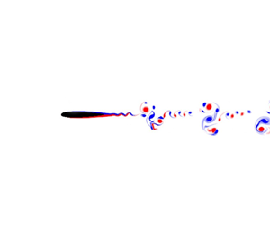
Figure 9. (a) Flow patterns in the  $DC\unicode{x2013} Sw$ plane. (b–g) Typical wake structures. Red and blue denote positive and negative vorticity, respectively.
By increasing  $Sw$ (by increasing either $A$ or $T$), a blurry flow pattern, i.e. Mode I and Mode II wakes, appears gradually at $DC \leq 0.5$. There are four types of vortex structures in the Mode I and Mode II wakes: A, B, C and D (figures 9e,f). The vortex structure A corresponds to the boundary layer separation in the gliding phase, forming nS and mP+nS structures in the Mode I and Mode II wakes, respectively (Williamson & Roshko Reference Williamson and Roshko1988). The vortex structures B, C and D are generated during the S-start phase. The vortex structure B in the Mode I and Mode II wakes is similar, where a strong positive vortex is surrounded by two weak negative vortices. The vortex structure C contains several negative vortices, with the Mode II wake providing more single vortex structures compared to the Mode I wake; see figure 9(f). The blurry vortex structure D describes the interaction between vorticity produced by the S-start phase and the one produced by the gliding phase. The evolution of Mode I and Mode II wakes due to the intermittent motion of a pitching foil has also been reported in Akoz et al. (Reference Akoz, Han, Liu, Dong and Moored2019), where it is mentioned that vortex structures B and D increase the swimming velocity, whereas structure C causes a deceleration. The Mode III wake occupies a large portion of the $DC$–
$DC$– $Sw$ plane. After a series of vortex mergers, the Mode III wake eventually becomes a 2P wake, as shown in figure 9(g).
4. Conclusions
In this work, intermittent S-start swimming is studied in a systematic manner. The numerical study reveals that the time-averaged swimming velocity  $\bar {U}_x$ and the cost of transport $CoT$ increase with decreasing duty cycle $DC$. This suggests that although intermittent S-start swimming leads to higher swimming speeds (which is good for both escaping predators and striking prey), it is an inefficient swimming gait compared to continuous cruising. We also presented two scaling laws to characterize the hydrodynamic performance of S-start swimmers, $Re \sim Sw^{4/3} /DC^{2/3}$ and $C_E \sim Sw^{5/3} /DC^{4/3}$, which are suitable for moderate speed flows ( $10^3 < Re < 10^5$) considered in this work. During swimming, hydrodynamic performance can be measured by $Re$ and $C_E$, which represent swimming speed and energy consumption. We can use $Sw$ and $DC$ to measure kinematic inputs for the swimmer. At high $Re > 10^6$, we expect the hydrodynamic performance metrics to scale as $Re \sim Sw/ DC^{1/2}$ and $C_E \sim Sw^{2}/ DC^{3/2}$, although this needs to be verified. Additionally, we also classified the wake structures of self-propelling intermittent S-start swimmers in this work. Finally, we note that the plots relating to scaling results appear to be stratified according to $DC$: points with higher $DC$ values lie beneath points with lower $DC$ values. A similar stratification is also found in the work of Akoz & Moored (Reference Akoz and Moored2018) (see their figure 10). Perhaps the scaling relations do not quite capture $DC$ effects, and this motivates further investigation.
Supplementary movie
A supplementary movie is available at https://doi.org/10.1017/jfm.2024.103.
Acknowledgements
The authors thank the anonymous reviewers for their insightful comments and careful analysis of the scaling laws, which improved this work.
Funding
J.W. acknowledges the support of the National Natural Science Foundation of China (grant no. 12072158) and the Natural Science Foundation of Jiangsu Province (grant no. BK20231437). This work is also supported by the Priority Academic Program Development of Jiangsu Higher Education Institutions (PAPD). K.K. and A.P.S.B. acknowledge the support of United States National Science Foundation Award OAC 1931368.
Declaration of interests
The authors report no conflict of interest.


